Modeling and Resource Allocation for Mobile Video over WiMAX

354

IEEE JOURNAL ON SELECTED AREAS IN COMMUNICATIONS, VOL. 28, NO. 3, APRIL 2010

Modeling and Resource Allocation for Mobile Video over WiMAX Broadband Wireless Networks Abdel Karim Al Tamimi, Student Member, IEEE, Chakchai So-In, Student Member, IEEE, and Raj Jain, Fellow, IEEE

Abstract—The key to proper resource allocation for mobile video on wireless networks is to have a good model for the resource demands. In this paper, we present the results of analysis of a number of mobile video streams and show that a simple seasonal ARIMA model (SAM) can provide a very good representation for both MPEG4-Part2 and MPEG4-Part10 videos, the formats that are commonly used for mobile videos. The model has been implemented to provide both video frame and RTP packet generators. The model can be used to represent different movies and can be easily adjusted to produce different workloads for simulation studies. We use the SAM generator to compare the performance of three different scheduling methods for video over WiMAX networks: Earliest Deadline First (EDF), Deficit Round Robin (DRR) and a combination of the two. The results show that under overload, EDF introduces unfairness. DRR with deadline is fair and gives the best performance. Index Terms—Video Modeling, Seasonal ARIMA, Traffic Generator, Earliest Deadline First, Deficit Round Robin, Mobile WiMAX, IEEE 802.16e, Scheduling, Resource Allocation, QoS.

I. I NTRODUCTION

M

OBILE video is considered as a major upcoming application and revenue generator for broadband wireless networks such as those based on WiMAX or LTE. It is important to design proper resource allocation schemes for mobile video since video is both throughput consuming and delay sensitive. In order to compare resource allocation for mobile video, it is important to have an accurate model of the traffic generated by mobile videos. In this paper, we present the results of analysis of several mobile video traces. The two compressions standards that are most commonly used for mobile video are: MPEG-4 Part 2 and MPEG-4 Part 10. We analyzed both types of traces and found that a simple Seasonal ARIMA (auto-regressive integrated moving average) model can be used to represent many different movies. The simple Seasonal ARIMA (SAM) model was used to develop a frame generator program that can be used in simulation and modeling studies. The details of the generator are presented in this paper. We use the generator to compare three resource allocation schemes for mobile video streaming over WiMAX networks. We investigated three scheduling algorithms: Earliest Deadline First (EDF), Deficit Round Robin (DRR) and a combination of EDF and DRR. The fairness and Manuscript received 1 March 2009; revised 1 November 2009. A. Al Tamimi, C. So-In, and R. Jain are with the Department of Computer Science and Engineering, Washington University in St. Louis, St. Louis,MO, 63130 USA (e-mail: aa7,cs5,jain @cse.wustl.edu). Digital Object Identifier 10.1109/JSAC.2010.100407.

packet loss due to deadline control for the three algorithms are compared. II. M OBILE V IDEO M ODELING Moving Picture Expert Group (MPEG) standard MPEG-4 Part 2 is one of the most commonly used video compression methods for mobile video. The new MPEG-4 Part10 and what is commonly known as Advanced Video Codec (AVC) is another vital player in the mobile video streams world. Though this standard provides a better compression rate and a smaller mean frame size, it also results in a higher variation of frame sizes than its predecessors. This makes the resource allocation problem more complicated and even harder to achieve reasonable results with simple approaches. Mobile videos are different from other videos in their encoding settings, such as: the video resolution (screen size), and the assumed decoding power on the targeted device, which in return restrict the use of the encoding methods in the encoding process. For further information about these standards and their characteristics the reader can refer to [1,2]. Many different statistical methods have been used to model video traffic. One of the first approaches was using Markov chain models [3-5], which are known for their inefficiency of representing the characteristics of MPEG traffic and their requirements of numerous states to achieve a desired accuracy. Complex models like wavelet models [6] have been also proposed. In addition to their complexity, wavelet models have been found be less accurate than other models [7]. Seasonal time series models like autoregressive integrated moving average (ARIMA) have been used to model GSM traffic [8]. Fractional ARIMA has been used to capture the long range dependence (LRD) between video frames, but these efforts were later abandoned because of their implementation complexity and the marginal improvements that they provided [8, 11]. Many of the models mentioned above used short movie scenes; which raises questions about their applicability to long traces. In addition, some of the models either have quite complex procedures to generate video frames, or require up to thousand of coefficients in order achieve the desired level of accuracy [9, 25]. The lack of good statistical models for video traffic resulted in many researchers using a trace-driven approach, which is limited by the amount of traces to which the researchers can have access. There are also issues about the portability, usability and accuracy of analysis results since the results may be related to specific movies.

c 2010 IEEE 0733-8716/10/$25.00 

AL TAMIMI et al.: MODELING AND RESOURCE ALLOCATION FOR MOBILE VIDEO OVER WIMAX BROADBAND WIRELESS NETWORKS

Fig. 1.

355

Statistical Modeling Versus Trace-driven Simulation Approach

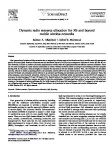
Trace-driven simulations are known for credibility. It is easy to convince others that the workload is representative. On the other hand, their finiteness and representativeness are questionable. In addition to that, it is hard to adjust any parameters of the trace or to extend it if there is a need for continuing simulations beyond the frames available in the trace file [10]. Fig. 1 shows the difference between the two approaches. Statistical traffic models are considered a better workload choice, since they provide a better understanding of the tradeoffs of various traffic parameters. Many of the statistical models are cursed with complexity and require a significant amount of time to verify and implement. Once a representative model is obtained, it is easy to be changed and adapted to different workload parameters. A. Introducing the SAM Model MPEG videos frames are known to have seasonal characteristics. As shown in the Fig. 2, MPEG video frames are divided into three types: I, P, and B frames. They differ in their function and in their size. While I frames have the biggest sizes, B frames have the smallest sizes of them all. The pattern of video frames is repeated every “s” frames where s is the Group of Pictures (GOP) size. This observation justifies our approach to model MPEG videos as a time series model. Our goal was to find a simple yet accurate model that is applicable to any MPEG video. We used an auto-regression integrated moving average model (ARIMA) because it is known to be a general model and it is relatively simple to implement compared to other approaches. In addition to that, ARIMA models are known to have a good accuracy in predicting future values. This feature allows researchers to improve admission control and scheduling mechanisms and optimize resource usage.For more information regarding ARIMA and its characteristics, the reader can refer to [11,14-16,32]. Because of the complexity of MPEG video patterns, other researchers have pointed out that a better approach to the problem is to use a multiplexed model or what is also known as a composite IPB model [12,13]. In this model, the video frame sequence is divided in to three sequences of I, P, and B type frames and each sequence is modeled separately. During generation, three streams are generated and then combined to form the final MPEG video trace. The individual models representing each frame stream are simpler than a single allframes model. Though this approach produces slightly better results than the one or all-frames model, each movie trace needs to be analyzed three times in order to produce the needed traces. We started our analysis by modeling simple advertisement videos of 15-30 seconds. All the videos that

Fig. 2.

Seasonal Characteristics of MPEG Video

we tested were encoded specifically for mobile devices. Our first concern was to verify the claim that IPB model is better than an all-frames model [12,13]. We expanded our initial set of video samples to include short movie scenes that had around 6000 frames. Our results, presented in Table I, confirmed that IPB model is slightly more accurate, but we found that the improvement is not justifiable given the extra efforts needed to analyze and implement three different streams. We measured the goodness of a model using the commonly used Akaike’s Information Criterion or AIC [32], which takes into consideration both the complexity of the model and its accuracy. Lower AIC index values indicate better models. Through our analysis we also noticed that although the optimal model for each trace was different, a particular simple model was very close to optimal in all cases. We call this model: Simplified Seasonal ARIMA Model or SAM [20]. SAM can be represented as follows: SAM = (1, 0, 1) × (1, 1, 1)s

(1)

The model has an auto-regression of order 1, integration of order 0, moving average of order 1 or ARIMA(1, 0, 1). There is a seasonal period of s, where s is the GOP size. The seasonal part itself has an auto-regressive part of order 1, integrated part of order 1, and moving average part of order 1 or ARIMA(1, 1, 1). Similar models have been used to model airline data [17]. SAM is a very simple model that requires only 4 parameters to represent a movie trace, in addition to the standard deviation of the modeling errors. Table I shows the AIC for three movies using the optimal all-frames model, optimal composite (I-P-B) model, and the SAM model. Note that the composite model gives the best results. However, the difference between the optimal composite model and all-frames model is less than 1%. The SAM model is similarly close to the optimal allframes model. The difference is less than 0.1%. The advantage of SAM model is that we can use this one model for all movies. B. Modeling MPEG-4 Part 2 Video Traces The next step of our analysis was to confirm our results using random scenes from different movies. We confirmed that the chosen model is capable of modeling the selected scenes well. In addition to that, we noticed that scenes from similar movie genre can be represented by similar parameters values.

356

IEEE JOURNAL ON SELECTED AREAS IN COMMUNICATIONS, VOL. 28, NO. 3, APRIL 2010

TABLE I A LL -F RAMES M ODEL VS . C OMPOSITE M ODEL VS . SAM M ODEL R ESULTS Movie Matrix I LOTR I LOTR II

Model AIC (Akaike Info. Criterion) Model AIC (Akaike Info. Criterion) Model AIC (Akaike Info. Criterion)

All-Frames Model

Composite Model (I-Frames), (P-Frames), (B-Frames)

SAM Model

(3, 0, 1) × (1, 1, 1)12 1203693 (1, 0, 1) × (1, 1, 1)12 125689.7 (3, 0, 3) × (1, 1, 1)12 127488.4

(0, 1, 3), (1, 1, 1), (3, 1, 6) 119775.3 (0, 1, 5), (0, 1, 1), (2, 1, 2) 125270.9 (0, 1, 3), (0, 1, 1), (1, 1, 2) 125278.9

(1, 0, 1)] × (1, 1, 1)12 120378.1 (1, 0, 1)] × (1, 1, 1)12 125689.7 (1, 0, 1)] × (1, 1, 1)12 127597

TABLE II S TATISTICAL A NALYSIS OF V IDEO T RACES

TABLE III SAM M ODEL PARAMETERS FOR VARIOUS M OVIES

Movie

Standard Deviation

Mean

Variance

Hurst Index

LOTR 1 LOTR 2 LOTR 3 Matrix 1 Matrix 2 Matrix 3

9594.778 11178.38 10794.25 7946.338 10687.00 12701.56

9342.26 11481.00 11145.63 7348.922 9508.467 10522.08

92059757 124956269 116515800 63144295 114212020 161329728

0.9158 0.9158 0.9233 0.9011 0.9147 0.9253

This observation led us to the conclusion that several different movies can be represented with the same model values. We then repeated the analysis on entire movie sequences (not just short scenes) and confirmed that SAM model can be used to model entire movies. This means that our model is general and yet accurate to adhere to the changes of frame sizes that occur inside the movie trace due to scenes changes. Most of the used movie traces are available through [31]. We noticed that movies that have similar level of texture details and motion variation have similar model parameters. We have conducted our intensive analysis using several movie traces. Among these are the following six movies: the Matrix trilogy, and The Lord of the Ring trilogy. Table II shows the statistical characteristics of these movies. The mean and the variances of the frame sizes listed in Table II indicate that the six movies are quite different. However, these movies can all be well represented by the SAM model. Our results, as shown in Table III, show that the six movies have similar model parameters (autoregressive or AR, movingaverage or MA, seasonal autoregressive or SAR, and seasonal moving-average or SMA). The difference between these values is insignificant and it is less than 1%. This is the unique part of the SAM model that such diverse set of movies can be represented partially by a single set of parameters. While optimal seasonal ARIMA models for each of these movies are quite different and the parameters of the optimal models are quite different, the SAM model is simple and achieves performance very close to the optimal performance. Some of our analysis results are shown in Table IV, which lists mean absolute error (MAE), mean absolute relative error (MARE), inverse of signal to noise ratio (SNR−1 ), and normalized mean square error (NMSE) for the optimal model and the SAM model. Notice that on all these statistical measures, SAM is close to optimal.

Movie LOTR 1 LOTR 2 LOTR 3 Matrix 1 Matrix 2 Matrix 3

AR 0.93 0.93 0.93 0.92 0.94 0.94

MA -0.69 -0.68 -0.68 -0.66 -0.68 -0.64

SAR 0.24 0.27 0.27 0.16 0.23 0.10

SMA -0.86 -0.86 -0.84 -0.81 -0.88 -0.90

Mean [Min, Max] Abs [Max-Min] /Mean

0.93 [0.92,-0.94]

-0.67 [-0.69, -0.64]

0.21 [0.1,0.28]

-0.86 [-0.9,-0.81]

0.015

0.087

0.814

0.104

TABLE IV S TATISTICAL C OMPARISONS BETWEEN SAM AND O PTIMAL M ODELS

Movie LOTR 1 LOTR 2 LOTR 3 Matrix 1 Matrix 2 Matrix 3

Movie LOTR 1 LOTR 2 LOTR 3 Matrix 1 Matrix 2 Matrix 3 MAX Diff %

Optimal Model MAE MARE 1850.149 0.3256206 2038.680 0.2806260 1940.064 0.2889833 1553.833 0.3700388 2126.052 0.3839772 2830.622 0.3941804

MAE 1851.281 2043.132 1944.378 1553.584 2132.762 2845.982 0.5426%

SAM MARE 0.3240269 0.2799332 0.2888479 0.3694246 0.3864979 0.3957961 0.6565%

SNR−1 0.0848033 0.0708604 0.0685161 0.0957917 0.0993043 0.1267721

NMSE 0.1652013 0.1456091 0.1415653 0.177721 0.1779137 0.2137702

SNR−1 0.0848344 0.0709581 0.0686010 0.095829 0.0995010 0.1277827 0.7972%

NMSE 0.1652620 0.1458099 0.1417407 0.1777901 0.1782661 0.2154743 0.7972%

To see how SAM model match up to the original traces, we compared the auto-correlation function (ACF), cumulative distribution function (CDF), and full length traces with those of the frame sizes generated by the SAM model. The results, as shown in Fig. 3 for the LOTR-2 trace, demonstrate the accuracy of SAM model when compared to the original traces. We have shown in this section that SAM model is capable of capturing the statistic features of MPEG video traces. Similar movies with similar statistical characteristics have been shown to have similar parameter values. These results have encouraged us to pursue our analysis to analyzing movies encoded with other commonly used codec for mobile video.

AL TAMIMI et al.: MODELING AND RESOURCE ALLOCATION FOR MOBILE VIDEO OVER WIMAX BROADBAND WIRELESS NETWORKS

(a) Full Trace Length Comparison

(b) A Close Up Comparison

(a) ACF Comparison

(b) CDF Comparison

357

Fig. 3. SAM Model Results: LOTR 2 Movie

C. Modeling MPEG-4 Part10/AVC Video Traces MPEG-4 Part 10 or AVC is also known as H.264 standard. The standard has shown significant improvements over older codecs. AVC encoded movies have lower mean values compared to MPEG-4 Part 2 videos. This is due to the fact that AVC compression is more complex and thus on the down side it requires more processing power. Long range dependence (LRD) level between video frames has been recorded to be similar to MPEG videos. Because of the new techniques in AVC compression, the encoded videos have higher variability in their frame sizes. Therefore, an accurate model that can represent highly variable sizes of video frames is a nontrivial task. The reader can refer to [2] for more information. One of the main differences between MPEG Part 2 and AVC encoded videos is the multiple frame reference feature in AVC. This feature allows the picture frames to refer to intra-GOP reference frames, which indicates that the correlation between the frames is not contained in one GoP period. This results in the observed seasonality period changing from s to 2s where s is the GOP size. Fig. 4 shows the autocorrelation function (ACF) for AVC coded video. Notice that the repetition period is 2s. This observation led us to change our SAM model from its previous formula to the following formula. SAMAV C = (1, 0, 1) × (1, 1, 1)2s

(2)

Similar to our previous analysis, we tested several optimized models for AVC and compared them against the SAMAV C model. Our analysis shows that SAMAV C produces very good AIC values. Another way to describe SAM is to represent the seasonality of the model independently of the GoP size. We achieved this by using the interval between two consecutive maximum or peak ACF values instead. The interval value can be obtained easily visually or using simple mathematical

Fig. 4.

Seasonality in AVC Encoded Movies

approaches like comparing the maximum ACF values over a reasonable number of lags. We have also examined several encoding settings for AVC. The two main encoding attributes that we examined are: quantization level, and number of B frames inside one GOP. For GOP size of 16, we have tested the following B-frame numbers: 1, 3, and 7, and the following quantization levels: 10, 28, and 48. Changing the number of B frames results in changing the relationship among the frames which is reflected in the ACF plot. Changing the quantization level has a deep impact on the average frame size. As shown in Fig. 5, the mean frame size depends mainly on the quantization level rather than the number of B frames. Fig. 6 shows a comparison of frame sizes, ACF, and CDF of the frame trace and a sequence generated from the SAM model. Notice the SAM model is capable of capturing the statistical characteristics of the modeled data. Additionally, we have conducted a thorough research analysis of more than 50 AVC encoded video traces. The results are available

358

IEEE JOURNAL ON SELECTED AREAS IN COMMUNICATIONS, VOL. 28, NO. 3, APRIL 2010

TABLE V S TATISTICAL C OMPARISON B ETWEEN SAMAV C AND O PTIMAL M ODELS

MAE 0.089 0.144

Movie SOL Star Wars

MAE 0.487 0.509

SOL Star Wars

Model (1,1,1)×(0,1,2)16 (1,0,1)×(1,1,1)8

(a) Quantization Effect on Mean Frame Size

(b) Quantization Effect on ACF Fig. 5.

Quantization Level Effects on Video Frames

through our website [33].Table V shows a statistical comparison between SAM model and the optimal SARIMA models for two of the analyzed AVC encoded videos, Silence of the Lambs (SOL) and Star Wars IV. As shown in the results, the optimal models have in general better results, except in the AIC comparison, where SAM results are better. These AIC results reflect the simplicity of the SAM model. These results have encouraged us to implement a frame generator based on the SAM model. Our target is to create a video traffic generator that is accurate, efficient, and easy to use by other fellow researchers. The next section will describe our approach to implement the SAM traffic generator and the challenges that we faced on our way. III. SAM M OBILE V IDEO F RAME G ENERATOR Our analysis on all the movies was done using the open analysis package R [18]. R provides several tools to model and display the obtained results. To simulate our results we started using two tools provided by R: arima.sim function and gsarima package’s function garsim. Both functions can simulate ARIMA models but not seasonal ARIMA models. In order to proceed, we had to convert our ARIMA model to either abstracted AR, or MA models. This approach is well known to statisticians to simplify model simulations. For more information the readers can refer to [11,15]. Our choice to select AR model over MA model was based on the fact that it is easier to keep track of the old values generated by the simulator. In addition to that, after testing both AR and MA models, we noticed that MA coefficients values do not converge over time. This affects the simulation accuracy and its implementation applicability. By converting the SAM model to a series of AR coefficients, we were able

Optimal Model MARE SNR−1 0.461 1.75e-05 0.220 2.63e-05

Movie SOL Star Wars

SAM MARE 0.566 0.249

NMSE 0.074 0.111

SNR-1 9.59e-05 9.32e-05

NMSE 0.075 0.092

Model AIC 1032633 1039591

SAM AIC 1031891 1029442

to determine the desired level of accuracy and complexity of the model. For instance, the total number of AR coefficients for MPEG-4 Part-2 SAM model is 1650. Fig. 7 below shows the different levels of accuracy that corresponds to different numbers of used AR coefficients. From our analytical analysis and simulation results, we found that 250 AR coefficients are sufficient to provide an accurate simulation. SAM generator incorporates arrep function as a component of its implementation, which is a part of gsarima package. arrep is capable of converting ARIMA models to their representations as a series of AR coefficients. That allows the generator users to supply only the five parameters mentioned before, (i.e., four ARIMA parameters plus the standards deviation of error terms). The traffic generator is capable of generating any specific number of frames, and allows the user either to store the results into a file or to use the continuous stream as an inner layer for other applications. One of the challenges in writing the traffic generator is to imitate the randomness of the transition of the movie scenes. A straight forward implementation of the seasonal ARIMA model is capable of capturing the statistical relationships between the frames, but it cannot predict or simulate the random shocks in video frame sizes [34]. This is because the model represents a smoothed version of the modeled traces due to the differencing method used. These random shocks represent a sudden transition of video frame sizes, and show up as spikes in video traces. To overcome this problem, SAM traffic generator includes a simple mechanism that inserts random shocks into the video stream while guaranteeing that frame sizes to be within reasonable values (i.e. non-negative frame sizes). The mechanism starts by picking random points in the generated trace to be the center of the random shock representing 1% of the trace points. Then these points are multiplied by ten. The near surrounding points values are increased to allow a smoother transition to the center of the random shock. The farther surrounding points’ values are decreased in order to emphasis the sudden transition of the random shock, and to maintain the same mean frame size value over the entire movie trace. Fig. 8 shows a comparison between Matrix 1, Matrix 3 and a generated trace using the SAM traffic generator with random shocks. Another major concern in designing the SAM traffic generator was to ensure that in addition to the mean and range,

AL TAMIMI et al.: MODELING AND RESOURCE ALLOCATION FOR MOBILE VIDEO OVER WIMAX BROADBAND WIRELESS NETWORKS

Fig. 6.

(a) Full Trace Comparison

(b) A Close Up Comparison

(c) ACF Comparison

(d) CDF Comparison

359

Fig. 6. Modified SAM Model Results.

A. RTP Traffic Generator

Fig. 7. Different Accuracy Levels for Different Numbers of AR Coefficients.

the generated trace CDF (cumulative distribution function) is within the acceptable range of the other related movies. This should hold true for different trace period lengths. Fig. 9 shows our results of comparing the CDFs of SAM traffic generator traces against original movie traces for short length traces (5k frames), medium length traces (30k frames), and long traces (150k frames). The SAM traffic generator can generate any required number of frames and has a stable and reliable performance. We have conducted several trials. With non-optimized code under debug mode we were able to generate 500k frames in less than 6.7 seconds. The SAM traffic generator described so far produces frame sizes of video frames. In the next section we present the implementation details of SAM RTP traffic generator.

Our implementation of the SAM traffic generator allows users to integrate the generated frames with any protocol layer with ease. On most systems, these video frames are transmitted using real time transport protocol (RTP). RTP protocol is defined in RFC number 3550 [20]. In this section we present the details of our RTP packet generator based on the SAM model. RTP packetizing is a very simple mechanism and follows two simple rules: packets can carry data from one video frame only, and if frames are small in size, you can fit as many full frames as the packet size allows. We have tested the SAM RTP packet generator against RTP packets generated using original movie traces. The results have confirmed that the generated RTP packets share the same statistical characteristics. Fig. 10 shows the generated RTP packets from LOTR I movie trace and the SAM RTP packet generator with an MTU (maximum transmission unit) size of 1500. Since the same RTP packetizing method has been applied to both original and generated traces, that have been compared before, we have omitted the statistical comparison between the two traces to avoid redundancy. The SAM RTP packet generator is just an example of what can be integrated to the SAM traffic generator to meet any desired simulation conditions. Other protocols can be implemented as easily, which gives great opportunities to test different standards or custom protocols and to optimize network performance.

360

IEEE JOURNAL ON SELECTED AREAS IN COMMUNICATIONS, VOL. 28, NO. 3, APRIL 2010

Fig. 9. Fig. 8.

CDF Comparisons for Short, Medium and Long Traces.

Random Shocks Implementation in SAM Traffic Generator.

IV. R ESOURCE A LLOCATION IN M OBILE W I MAX N ETWORKS The main reason for our mobile video traffic modeling is to understand and optimize the performance of mobile video over WiMAX networks. In this section we present the results of our analysis of various scheduling methods for Mobile WiMAX networks using the SAM traffic generator. This analysis is to illustrate that SAM generator can be used to test and develop new and improved resource allocation schemes. Mobile WiMAX uses a fixed frame-based allocation. Basically, each frame is of 5 ms duration [21]. It starts with a downlink preamble and Frame Control Header (FCH) followed by a downlink (DL) map and an uplink (UL) map. These maps contain the information elements that specify the burst profile for each burst. The burst profile consists of burststart time, burst-end time, modulation type and Forward Error Control (FEC) used or to be used in the burst. All scheduling schemes discussed in this paper can be used for both frequency division duplexing (FDD) and time division duplexing (TDD) systems. However, to keep the discussion focused, we use TDD throughput this paper. Although the standard allows several configurations such as mesh networks and relay networks, our focus is only on point to multipoint network configuration. Thus, the resource

allocation problem is basically that the base station (BS) is the single resource controller for both uplink and downlink directions for each mobile station (MS). Each MS has an agreed quality of service (QoS) requirement that is negotiated between the BS and MS at the time of connection setup. The BS grants transmit opportunities to various MSs based on their bandwidth requests and QoS. In this experiment, we basically focus on how to allocate the number of slots for each MS in each Mobile WiMAX frame. Each slot consists of one subchannel allocated for the duration of some number of OFDM symbols. The number of subcarriers in the subchannel and the number of OFDM symbols in the slot depend upon the link direction (uplink or downlink) and the permutation scheme used. For example, in Partially Used Sub-Channelization (PUSC) permutation scheme, which is commonly used in Mobile WiMAX, one slot consists of one subchannel over two OFDM symbol periods for DL and one subchannel over three OFDM symbol periods for UL [22]. Mobile WiMAX supports several Modulation and Coding Schemes (MCSs), such as Binary Phase Shift Keying (BPSK) and several Quadrature Amplitude Modulation (QAM) schemes. BPSK results in 1 bit per symbol and is used for poor channel conditions. QAM schemes result in more bits per symbol and are used for reliable channel conditions. Since the MCS used for a mobile station depends upon the

AL TAMIMI et al.: MODELING AND RESOURCE ALLOCATION FOR MOBILE VIDEO OVER WIMAX BROADBAND WIRELESS NETWORKS

(a)Lord of The Rings I RTP Packets

(b)SAM RTP Packets Fig. 10.

361

the packet is not scheduled and the deficit (amount that would have been allocated) is remembered. However, to fully utilize a WiMAX frame, we use a modified version of DRR, DRR with fragmentation described in [24]. In general, if a packet meets the fair share limit, we schedule it in the current WiMAX frame and if necessary, allow the part that will not fit in the current WiMAX frame to be scheduled in the next frame. This ensures that WiMAX frame capacity is not wasted. Note that in order to overcome the issue of varying link capacity in Mobile WiMAX networks, the fair share is derived from the queue length and MCS level. Moreover, we use MaxMin fair algorithm to derive the fair share so that the left over space within Mobile WiMAX frame can be used. 3) Earliest Deadline First with Deficit Round Robin (EDFDRR): With EDF-DRR, we basically apply EDF first then regulate the packet stream with DRR. In other words, the packets are sorted according to the deadline then DRR is used to decide whether the packet with the earliest deadline is eligible for transmission without exhausting the flow’s credits (deficits). Again, we allow fragmented packets to be transmitted for frame utilization purpose.

RTP Generated Packets Using SAM-RTP Packet Generator

B. Scheduling Algorithms with enforced deadline location of the mobile station and varies with time, the slot capacity (number of bits in the slot) is not constant. Given equal number of slots, mobile stations at different locations may be allowed to use different MCSs, resulting in different resource allocations. In the study presented here, our focus is on fairness and delay among multiple users and so we assume all users to be in similar channel conditions. The main QoS parameters are the throughput and delay constraints. In Mobile WiMAX networks, a simple Earliest Deadline First (EDF) scheduling algorithm is generally used to schedule real-time traffic especially video traffic, and Deficit Round Robin (DRR) scheduling algorithm is commonly used to schedule non-real-time traffic [30,35-36] in downlink direction. We compared these two algorithms and a combination of the two.

For real-time traffic, video traffic in particular, received packets with huge delay or over the deadline are not useful. Since the deadline or average delay is negotiated during the connection setup, we can use the deadline information at the scheduler by dropping the packets that are over the deadline and save the bandwidth. Therefore, for all three algorithms described above packets are dropped if it will not meet the deadline after transmission. We analyzed cases without this option, however, the results showed worse performance with a large fraction of packets being discarded at the destination due to exceeding the deadline. We concluded that given the resource constrained nature of wireless medium, any reasonable implementation should minimize waste by discarding late packets before transmission. C. Performance Evaluation

A. Scheduling Algorithms In this section, we briefly describe the three scheduling algorithms. These are Earliest Deadline First (EDF), Deficit Round Robin (DRR) and Easiest Deadline First with Deficit Round Robin (EDF-DRR) in the context of mobile WiMAX networks. 1) Earliest Deadline First (EDF): Given a set of flows, the first algorithm, EDF [23] simply compares the packets at the head of the flow queues and schedules the packet the earliest deadline constraint. One additional complication in the case of WiMAX is that the entire packet may not fit in the current WiMAX frame and a fragment may be left over. These fragments are transmitted first in the next WiMAX frame. The entire packet is discarded if the fragment does not meet the deadline. 2) Deficit Round Robin (DRR): The second algorithm, DRR [24], avoids packet fragmentation by scheduling only a full packet. If a packet will result in exceeding the fair share,

In this section, we present simulation results of system throughput, delay, jitter, and fairness for EDF, EDF-DRR and DRR algorithms. We also show the results of those algorithms with deadline enforced. We consider only the downlink resource allocation. The simulation configuration and parameters follow the performance evaluation parameters specified in Mobile WiMAX System Evaluation document and WiMAX profiles [23, 28]. These parameters are briefly summarized in Table VI. With 10 MHz system bandwidth, 5 ms frame, 1/8 cyclic prefix and a DL:UL ratio of 2:1, the number of downlink symbol-columns per frame is 29 [22,27]. In PUSC mode, there are 30 subchannels and each slot consists of one subchannel over 2 symbol duration. As a result, there are 30 × (28/2) = 420 downlink slots per frame. Of these, 51 slots are required for Frame Control Header (FCH), DL MAP and UL MAP (repetition of 4 and QPSK-1/2) and Downlink Channel Descriptor (DCD) and Uplink Channel Descriptor (UCD) overheads assuming a case of five mobile stations.

362

IEEE JOURNAL ON SELECTED AREAS IN COMMUNICATIONS, VOL. 28, NO. 3, APRIL 2010

TABLE VI P ERFORMANCE E VALUATION PARAMETERS [23]

Parameters PHY Duplexing Mode Frame Length System Bandwidth FFT size Cyclic prefix length DL permutation zone RTG + TTG DL:UL ratio DL Preamble MAC PDU size ARQ and packing Fragmentation DL-UL MAPs

Values OFDMA TDD 5 ms 10 MHz 1024 1/8 PUSC 1.6 symbol 2:1 (29:18 OFDM symbols) 1 symbol-column Variable length Disable Enable Variable

TABLE VII S YSTEM T HROUGHPUT D ELAY AND D ELAY J ITTER WITH E NFORCED D EADLINE (5 F LOWS IN OVERLOAD S CENARIO)

MS 1 2 3 4 5 MS 1 2 3 4 5 MS 1 2 3 4 5

Fig. 11.

WiMAX Simulation Topology

In our analysis, interference is represented as a change of MCS. To keep it simple, the MCS level is constant over the simulation period. A lower bit rate MCS indicates more interference than a higher bit rate MCS. In this study, we use only one MCS for the entire movie. It is possible to extend this to a time varying interference, but it would require agreeing to a model for time variation and would create more questions than it would answer. Thus, we have left that for future study. We also selected QPSK-3/4 (9 bytes per slot) for all mobile stations. Therefore, the system throughput for five MSs is around 5.4 Mbps excluding UCD/DCD. Notice that the actual overheads depend on the number of actual burst allocations in both uplink and downlink and other management messages. 1) Simulation Configurations: We used a modified version of WiMAX Forum’s ns-2 simulator [26] in which a Mobile WiMAX module has been added [27]. There are three main simulation configurations in order to show the fairness among MSs and the delay constraint for all three algorithms. First, an under-load scenario with three video flows with 1.35 Mbps average rate each and one Constant Bit Rate (CBR) flow with 3 Mbps. The purpose of CBR flow is to measure the unused space in the frame. We treated the CBR flow as a lower priority so that the CBR flow acquires transmission opportunity only if there is any unused space in the WiMAX frame. Second an overload scenario with five video flows with 1.35 Mbps average rate each. Third, we used three video flows and one CBR flow; however, one of the video flows is not well-behaved, sending more traffic. For this overloading flow, we used the SAM traffic generator to generate a video stream with an average rate of 3.3 Mbps. Because of the overload,

Send (Mbps) 1.49 1.18 1.53 1.24 1.47 Send (Mbps) 1.49 1.18 1.53 1.24 1.47 Send (Mbps) 1.49 1.18 1.53 1.24 1.47

(A)EDF Receive (Mbps) 0.90 0.76 1.14 0.74 1.11 (B)DRR Receive (Mbps) 0.95 0.98 0.96 0.97 0.98 (C)EDF-DRR Receive (Mbps) 0.89 0.95 0.85 0.89 0.88

Delay (ms) 21.38 20.83 21.31 21.22 21.20

Jitter (ms) 1.80 2.07 1.79 1.83 1.75

Delay (ms) 18.65 16.27 19.03 16.91 18.28

Jitter (ms) 3.84 4.30 3.46 4.31 3.86

Delay (ms) 19.63 17.07 19.90 18.04 19.63

Jitter (ms) 3.08 4.26 3.24 4.04 3.06

CBR flow does not really get any transmission opportunities in this case. Although we use three to five flows to show the effect of fairness, the results are expected to be similar with more MSs and higher MCS levels. Note that the video frames were packetized and RTP, UDP, and IP headers overheads were added. All video flows’ deadlines were set to 20 ms. All simulations were run from 0 to 10 seconds with 5 seconds of traffic duration. There are ranging, registration and connection setup processes during the first 5 seconds. To quantify fairness, we used Jain Fairness Index [28], which is computed as follows: n n   xi )2 /n x2i f (x1 , x2 , ..., xn ) = ( i=1

(3)

i=1

Here xi is the throughput for ith MS and there are n MSs or n flows. In our simulations, n is 3 or 5. Fig. 11 shows the simulation topology. The link between BS and MSs is a bottleneck. At the BS, there is one queue for each MS and each queue is 100 packets long. 2) Simulation Results: In this section, we show system throughput, delay, delay jitter of EDF, DRR and EDF-DRR with and without enforced deadline. For the first scenario, all algorithms (with and without enforced deadline) result in the same throughput, 1.5, 1.24 and 1.49 Mbps with 1.19 Mbps for CBR. There are no dropped packets for video flows. The average delay ranges from 6 to 7 ms. Table VII shows the results for the second overload scenario with deadline enforcement. Because of the deadline enforcement, average delays for all three algorithms are within the specified deadline of 20 ms plus 5 ms additional transmission delays (duration of the WiMAX frame). EDF is unfair, while DRR and EDFDRR are fair. The degree of fairness of DRR is a bit higher

AL TAMIMI et al.: MODELING AND RESOURCE ALLOCATION FOR MOBILE VIDEO OVER WIMAX BROADBAND WIRELESS NETWORKS

363

TABLE VIII S YSTEM T HROUGHPUT, D ELAY AND D ELAY J ITTER WITH E NFORCED D EADLINE (2 W ELL - BEHAVED F LOW AND O NE I LL - BEHAVED F LOW IN OVERLOAD S CENARIO)

MS 1 2 3 MS

Send (Mbps) 1.49 1.24 3.33

1 2 3

Send (Mbps) 1.49 1.24 3.33

1 2 3

1.49 1.24 3.33

(A)EDF Receive (Mbps) 1.19 1.03 2.66 (B)DRR Receive (Mbps) 1.49 1.24 2.34 (C)EDF-DRR 1.49 1.24 2.34

Delay (ms) 20.41 20.16 21.28

Jitter (ms) 1.93 1.99 1.83

Delay (ms) 9.69 8.70 20.58

Jitter (ms) 3.33 3.05 2.87

9.80 9.07 20.62

3.72 3.41 2.77

(a) EDF

than EDF-DRR, 0.9998 versus 0.9986, respectively. Fig. 12 also shows the system throughput for all three algorithms over time. Table VIII and Fig. 13 show the results for case with one ill-behaved flow. Deadline is enforced for all flows. Again, EDF cannot maintain the share for well-behaved flows. On the other hands, DRR and EDF-DRR can achieve Max-Min fairness for all flows. V. C ONCLUSIONS AND F UTURE W ORK The key contributions of this paper are as follows: 1) We show that seasonal ARIMA models can be used to accurately model both codecs commonly used for mobile video: MPEG-4 Part 2, and MPEG-4 Part 10/AVC/H.264. 2) Although a composite model with separate I-P-B streams is more accurate than a combined all-frames model, the complexity is not worth the 1% gain in accuracy. 3) Although optimal seasonal ARIMA models for different movies are very different, one simple model (1, 0, 1)×(1,1,1)s can be used to represent a variety of movies with MPEG-4 Part 2 encodings. Here, s is the GOP size used in the encoding. We call this model Simple seasonal ARIMA model or SAM. 4) In our analysis, we compare : a) Our SAM model b) Original Trace c) Other ARIMA models (through analysis) d) Other non-time series models we have shown that A is close to B and is simpler than C. Both C and D have the property that they are movie and scene specific and therefore more difficult to use. 5) Another strength of the SAM model is that the parameter values are very similar for the set of movies that belong to the same movie genre. 6) SAM model was found to apply to various scenes traces as well as to complete movies traces. 7) SAM also applies to movies encoded with MPEG-4 part 10 but the seasonal period is 2s where s is the size of

(b) DRR

(c) EDF-DRR Fig. 12.

System Throughput ( Five Video Flows in Overload Scenario).

the GOP. 8) A video frame generator has been developed based on SAM model. The key issue in the development of the generator was implementation of random shocks that simulates scene changes observed in actual movies. The generator allows easy adjustment of traffic parameters such as average frame rate, average frame size, standard deviation of errors etc. The model is available from the authors for open use. 9) A RTP packet generator addition to the SAM traffic generator allows producing packet traffic suitable for use

364

IEEE JOURNAL ON SELECTED AREAS IN COMMUNICATIONS, VOL. 28, NO. 3, APRIL 2010

DRR is fair and provides the best performance for realtime mobile video traffic. Although we have analyzed several advertisement videos, several video scenes, and several movies, there is always a need for analysis of more movies and we hope to continue this effort in future for mobile videos of other types. Similarly, resource allocation studies need to be continued for other topologies, varying MCS levels, different user configurations, with and without ARQ and H-ARQ [31]. R EFERENCES (a) EDF

(b) DRR

(c) EDF-DRR Fig. 13. System Throughput ( Two Well-behaved Video Flows and One Ill-behaved Flow in Overload Scenario).

in performance studies of mobile video. 10) The SAM frame generator was used to study the resource allocation in a mobile WiMAX network using WiMAX Forum’s NS-2 model and WiMAX Forum’s system evaluation guidelines. 11) Given the resource constrained nature of the wireless medium, for mobile video and other real-time traffic, it is important to discard packets that exceed the deadline before transmission on the wireless medium. 12) The simulation results for EDF, DRR, and EDF-DRR show that EDF is most unfair, EDF-DRR is less unfair.

[1] G. Van der Auwera, P. David, M. Reisslein, “Traffic characteristics of H.264/AVC variable bit rate video,” IEEE Communications Magazine, Volume 46 Issue 11, pp 164-174 [2] P. Seeking, M. Reisslein, and B. Kulapala, “Network Performance Evaluation with Frame Size and Quality Traces of Single-Layer and Two-Layer Video: A Tutorial”, IEEE Communications Surveys and Tutorials, Vol. 6, No. 3, Third Quarter 2004, pp. 58-78. [3] A.M. Dawood, M. Ghanbari “Content-Based MPEG Video Traffic Modeling,” IEEE Transactions on Multimedia, Volume 1, Issue 1, Mar 1999, pp. 77-87. [4] Y. Sun, J.N. Daigle, “A Source Model of Video Traffic Based on FullLength VBR MPEG4 Video Traces,” IEEE Global Telecommunications Conference, 2005. GLOBECOM’05, Volume 2, 28 Nov.-2 Dec. 2005, 5 pp. [5] O. Lazaro, D. Girma, and J. Dunlop “H.263 Video Traffic Modeling for Low Bit Rate Wireless Communication,” 15th IEEE International Symposium on Personal, Indoor and Mobile Radio Communications, 2004. PIMRC 2004. Volume 3, Issue, 5-8 Sept. 2004, pp. 2124-2128. [6] O.Lazaro, D. Girma, J. Dunlop, “Real Time Generation Of Synthetic MPEG-4 Video Traffic Using Wavelets,” Proceedings of IEEE VTS 54th Vehicular Technology Conference, Fall 2001 (VTC 2001),Volume 1, pp. 418 - 422. [7] O. Lazaro, D. Girma, J. Dunlop “A Study of Video Source Modeling for 3G Mobile Communication Systems,” Proceedings of First International Conference on 3G Mobile Communication Technologies, 2000, Conf. Publ. No. 471, pp. 461-465 [8] Y. Shu, M. Yu, J. Liu, and O.W.W. Yang “Wireless Traffic Modeling and Prediction Using Seasonal ARIMA Models,” Proceedings of ICC’03, Volume 3, 11-15 May 2003, pp. 1675-1679. [9] X. Huang, Y. Zhou, R. Zhang, “A Multiscale Model for MPEG-4 Varied Bit Rate Video Traffic,” IEEE transactions on broadcasting. Volume:50, Issue: 3, pp. 323- 334. [10] R. Jain, “The Art of Computer Systems Performance Analysis: Techniques for Experimental Design, Measurement, Simulation, and Modeling,” Wiley 1991. 685 pages [11] C. Chatfield, “The Analysis of Time Series: An Introduction,” Chapman & Hall/CRC, 6th Edition, 2003. 352 pages [12] N. Ansari, H. Liu, Y. Q. Shi, H. Zhao, “On Modeling MPEG Video Traffic,” IEEE Transactions on Broadcasting 2002, vol. 48, no 4, pp. 337-347 [13] M. Krunz, H. Hughes, “A traffic model for mpeg-coded VBR streams”, Proc. of the ACM SIGMETRICS/PERFORMANCE ’95 Conference , Ottawa, Ontario, Canada 1995, pp 47 - 55. [14] B. Nau, “Duke University, Decision 411 Course,” Duke University, URL=[http://www.duke.edu/˜rnau/Decision411CoursePage.htm],Feb09. [15] D. C. Montgomery, L. A. Johnson, J. S. Gardiner, “Forecasting and Time Series Analysis”, Second Edition, McGraw-Hill Companies; 2 Sub edition (July 1990), 381 pages. [16] G. Box, G. Jenkins, G. Reinsel,”Time series analysis forecasting and control,” Prentice Hall; 3rd edition (February 28, 1994), 592 pages. [17] J. Aston, et al., “New ARIMA Models for Seasonal Time Series and Their Application to Seasonal Adjustment and Forecasting”, placecountry-regionU.S. Census Bureau, Research Report, October, 2007 [18] R project, “The project R of statstical computing,” URL=[http://www.rproject.org/], Feb-28-2009. [19] A. Al Tamimi, R. Jain, C. So-In, “SAM: A Simplified Seasonal ARIMA Model for placeMobile Video over Wireless Broadband Networks”, IEEE International Symposium on Multimedia 2008, pp 178-183. [20] RFC-3550, “RTP: A Transport Protocol for Real-Time Applications”. July 2003 [21] IEEE P802.16Rev2/D2, “DRAFT Standard for Local and metropolitan area networks,” Part 16: Air Interface for Broadband Wireless Access Systems, Dec. 2007, 2094 pp.

AL TAMIMI et al.: MODELING AND RESOURCE ALLOCATION FOR MOBILE VIDEO OVER WIMAX BROADBAND WIRELESS NETWORKS

[22] WiMAX Forum, “WiMAX System Evaluation Methodology V2.1,” Jul. 2008, 230 pp. [http://www.wimaxforum.org/technology/documents] [23] M. Shreedhar, G. Varghese, “Efficient fair queueing using deficit round robin,” in Proc. ACM SIGCOMM Communication Review, 1995, vol 25, no. 4, pp. 231-242. [24] C. So-In , R. Jain, A. Al Tamimi, “A Deficit Round Robin with Fragmentation Scheduler for IEEE 802.16e Mobile WiMAX,” in Proc. IEEE Sarnoff Symposium., 2009, pp. 1-7. [25] L.J. De La Cruz, E. Pallares, J.J Alins, J. Mata, “Self-similar traffic generation using a fractional ARIMA model.Application to the VBR MPEG video traffic,” ITS ’98 Proceedings. SBT/IEEE Telecommunications Symposium 1998, vol 1, pp 102-107 [26] UCB/LBNL/VINT, “Network Simulator - ns (version 2),” Jun. 2007. URL=[http://www.isi.edu/nsnam/ns/index.html] [27] WiMAX Forum, “The Network Simulator NS-2 MAC+PHY Add-On for WiMAX,” Aug. 2007. Available to WiMAX Forum members. [28] R. Jain, D.M. Chiu, and W. Hawe, “A Quantitative Measure of Fairness and Discrimination for Resource Allocation in Shared Systems,” in DEC Research Report TR-301, 1984, 38 pp. [29] M. Andrews, “Probabilistic end-to-end delay bounds for earliest deadline first scheduling,” in Proc. IEEE Computer Communication Conf., Israel, 2000, vol. 2, pp. 603-612 [30] C. So-In, R. Jain, A. Al Tamimi, “Scheduling in IEEE 802.16e WiMAX Networks: Key Issues and a Survey,” in IEEE Journal on Selected Areas in Comm., vol. 27, no. 2, pp. 156-171, Feb. 2009, [31] Mobile video traces, “Mobile Devices: Video Traces, Arizona State University (ASU) and Aalborg University (AAU),” URL = [http://mobiledevices.kom.aau.dk/research/traffic and channel measurements/video traces/]. Feb-28-2009 [32] R. S. Tsay , “Analysis of Financial Time Series”, Wiley-Interscience, 1st edition (October 15, 2001). 472 pages [33] Modeling and Generating Video Traces using SAM website, URL=[ http://www.cse.wustl.edu/˜jain/sam/] [34] ARMA defnintion from the business dictionary , URL = [http://www.businessdictionary.com/definition/autoregressive-movingaverage-ARMA-model.html] [35] R. Jain, C. So-In, A. Al Tamimi, “System Level Modeling of IEEE 802.16e Mobile WiMAX Networks: Key Issues,” in IEEE Wireless Comm. Mag., vol. 15, no. Oct. 2008. [36] B. Kim, C. So-In,J. Yun, R. Jain, Y. Hur, A. Al Tamimi, “Capacity Estimation and TCP Performance Enhancement over Mobile WiMAX ,” IEEE Wireless Comm. Mag., vol. 47, no. 6, pp. 132-141, Jun. 2009

365

Abdel Karim Al Tamimi is currently a PhD candidate in Computer Engineering at Washington University in St. Louis, MO. Abdel Karim received his BA degree in computer engineering from Yarmouk University, Jordan. He has been awarded a full scholarship to peruse his Master and PhD degrees in computer engineering at Washington University in St. Louis, where he obtained his master degree [2007].

Chakchai So-In received the B.Eng. and M.Eng. degrees in computer engineering from Kasetsart University, Bangkok, Thailand in 1999 and 2001 respectively. He is currently working toward a Ph.D. degree at the Department of Computer Science and Engineering, Washington University in St. Louis, MO, USA.

Raj Jain is a Professor of Computer Science and Engineering at Washington University, St. Louis, MO. Dr. Jain is a Fellow of IEEE, a Fellow of ACM. He is the author of “Art of Computer Systems Performance Analysis, which won the 1991 “BestAdvanced How-to Book, Systems” award from Computer Press Association. His fourth book entitled “ High-Performance TCP/IP: Concepts, Issues, and Solutions,” was published by Prentice Hall in 2003. He is also a winner of ACM SIGCOMM Test of Time award and CDAC-ACCS Foundation Award 2009.