and w(m) is a vector white Gaussian noise with mean 0 and covariance ...... den, âCognitive engine implementation for wireless multicarrier transceivers,â Wiley ..... [69] B. Hilburn, T. R. Newman, and T. Bose, âSector-based policy generation ...
MODELING, FORECASTING AND RESOURCE ALLOCATION IN COGNITIVE RADIO NETWORKS by LUTFA AKTER B.S., Bangladesh University of Engineering and Technology, 2002 M.S., Bangladesh University of Engineering and Technology, 2004
AN ABSTRACT OF A DISSERTATION submitted in partial fulfillment of the requirements for the degree DOCTOR OF PHILOSOPHY Department of Electrical and Computer Engineering College of Engineering KANSAS STATE UNIVERSITY Manhattan, Kansas 2010
Abstract With the explosive growth of wireless systems and services, bandwidth has become a treasured commodity. Traditionally, licensed frequency bands were exclusively reserved for use by the primary license holders (primary users), whereas, unlicensed frequency bands allow spectrum sharing. Recent spectrum measurements indicate that many licensed bands remain relatively unused for most of the time. Therefore, allowing secondary users (users without a license to operate in the band) to operate with minimal or no interference to primary users is one way of sharing spectrum to increase efficiency. Recently, Federal Communications Commission (FCC) has opened up licensed bands for opportunistic use by secondary users. A cognitive radio (CR) is one enabling technology for systems supporting opportunistic use. A cognitive radio adapts to the environment it operates in by sensing the spectrum and quickly decides on appropriate frequency bands and transmission parameters to use in order to achieve certain performance goals. A cognitive radio network (CRN) refers to a network of cognitive radios/secondary users. In this dissertation, we consider a competitive CRN with multiple channels available for opportunistic use by multiple secondary users. We also assume that multiple secondary users may coexist in a channel and each secondary user (SU) can use multiple channels to satisfy their rate requirements. In this context, firstly, we introduce an integrated modeling and forecasting tool that provides an upper bound estimate of the number of secondary users that may be demanding access to each of the channels at the next instant. Assuming a continuous time Markov chain model for both primary and secondary users activities, we propose a Kalman filter based approach for estimating the number of primary and secondary users. These estimates are in turn used to predict the number of primary and secondary users in a future time instant. We extend the modeling and forecasting framework to the
case when SU traffic is governed by Erlangian process. Secondly, assuming that scheduling is complete and SUs have identified the channels to use, we propose two quality of service (QoS) constrained resource allocation frameworks. Our measures for QoS include signal to interference plus noise ratio (SINR) /bit error rate (BER) and total rate requirement. In the first framework, we determine the minimum transmit power that SUs should employ in order to maintain a certain SINR and use that result to calculate the optimal rate allocation strategy across channels. The rate allocation problem is formulated as a maximum flow problem in graph theory. We also propose a simple heuristic to determine the rate allocation. In the second framework, both transmit power and rate per channel are simultaneously optimized with the help of a bi-objective optimization problem formulation. Unlike prior efforts, we transform the BER requirement constraint into a convex constraint in order to guarantee optimality of resulting solutions. Thirdly, we borrow ideas from social behavioral models such as Homo Egualis (HE), Homo Parochius (HP) and Homo Reciprocan (HR) models and apply it to the resource management solutions to maintain fairness among SUs in a competitive CRN setting. Finally, we develop distributed user-based approaches based on “Dual Decomposition Theory” and “Game Theory” to solve the proposed resource allocation frameworks. In summary, our body of work represents significant ground breaking advances in the analysis of competitive CRNs.
MODELING, FORECASTING AND RESOURCE ALLOCATION IN COGNITIVE RADIO NETWORKS by LUTFA AKTER B.S., Bangladesh University of Engineering and Technology, 2002 M.S., Bangladesh University of Engineering and Technology, 2004
A DISSERTATION submitted in partial fulfillment of the requirements for the degree DOCTOR OF PHILOSOPHY Department of Electrical and Computer Engineering College of Engineering KANSAS STATE UNIVERSITY Manhattan, Kansas 2010
Approved by:
Major Professor Balasubramaniam Natarajan
Copyright Lutfa Akter 2010
Abstract With the explosive growth of wireless systems and services, bandwidth has become a treasured commodity. Traditionally, licensed frequency bands were exclusively reserved for use by the primary license holders (primary users), whereas, unlicensed frequency bands allow spectrum sharing. Recent spectrum measurements indicate that many licensed bands remain relatively unused for most of the time. Therefore, allowing secondary users (users without a license to operate in the band) to operate with minimal or no interference to primary users is one way of sharing spectrum to increase efficiency. Recently, Federal Communications Commission (FCC) has opened up licensed bands for opportunistic use by secondary users. A cognitive radio (CR) is one enabling technology for systems supporting opportunistic use. A cognitive radio adapts to the environment it operates in by sensing the spectrum and quickly decides on appropriate frequency bands and transmission parameters to use in order to achieve certain performance goals. A cognitive radio network (CRN) refers to a network of cognitive radios/secondary users. In this dissertation, we consider a competitive CRN with multiple channels available for opportunistic use by multiple secondary users. We also assume that multiple secondary users may coexist in a channel and each secondary user (SU) can use multiple channels to satisfy their rate requirements. In this context, firstly, we introduce an integrated modeling and forecasting tool that provides an upper bound estimate of the number of secondary users that may be demanding access to each of the channels at the next instant. Assuming a continuous time Markov chain model for both primary and secondary users activities, we propose a Kalman filter based approach for estimating the number of primary and secondary users. These estimates are in turn used to predict the number of primary and secondary users in a future time instant. We extend the modeling and forecasting framework to the
case when SU traffic is governed by Erlangian process. Secondly, assuming that scheduling is complete and SUs have identified the channels to use, we propose two quality of service (QoS) constrained resource allocation frameworks. Our measures for QoS include signal to interference plus noise ratio (SINR) /bit error rate (BER) and total rate requirement. In the first framework, we determine the minimum transmit power that SUs should employ in order to maintain a certain SINR and use that result to calculate the optimal rate allocation strategy across channels. The rate allocation problem is formulated as a maximum flow problem in graph theory. We also propose a simple heuristic to determine the rate allocation. In the second framework, both transmit power and rate per channel are simultaneously optimized with the help of a bi-objective optimization problem formulation. Unlike prior efforts, we transform the BER requirement constraint into a convex constraint in order to guarantee optimality of resulting solutions. Thirdly, we borrow ideas from social behavioral models such as Homo Egualis (HE), Homo Parochius (HP) and Homo Reciprocan (HR) models and apply it to the resource management solutions to maintain fairness among SUs in a competitive CRN setting. Finally, we develop distributed user-based approaches based on “Dual Decomposition Theory” and “Game Theory” to solve the proposed resource allocation frameworks. In summary, our body of work represents significant ground breaking advances in the analysis of competitive CRNs.
Table of Contents Table of Contents
viii
List of Figures
xi
List of Tables
xiv
Acknowledgements
xv
Dedication
xvi
1 Introduction 1.1 Cognitive Radio Networks . . . . . . . 1.2 Challenges in CRNs and Prior Work . 1.2.1 Spectrum Sensing . . . . . . . . 1.2.2 Resource Allocation . . . . . . . 1.2.3 Fairness in Resource Allocation 1.3 Motivation and Overview . . . . . . . . 1.4 Contributions . . . . . . . . . . . . . . 1.5 Organization . . . . . . . . . . . . . .
. . . . . . . .
. . . . . . . .
. . . . . . . .
2 Spectrum Usage Modeling and Forecasting 2.1 System Model . . . . . . . . . . . . . . . . . 2.2 Estimation of Spectrum Usage . . . . . . . . 2.3 Forecasting Spectrum Usage . . . . . . . . . 2.3.1 Forecasting Spectrum Usage of SU . 2.3.2 Forecasting Spectrum Usage of PU . 2.4 Experimental Results . . . . . . . . . . . . . 2.4.1 Simulated CRN . . . . . . . . . . . . 2.4.2 Measured Data Analysis . . . . . . . 2.5 SU Generalized Traffic Model . . . . . . . . 2.5.1 System Model . . . . . . . . . . . . . 2.5.2 Estimation of Spectrum Usage . . . . 2.5.3 Forecasting Spectrum Usage . . . . . 2.5.4 Experimental Results . . . . . . . . . 2.6 Summary . . . . . . . . . . . . . . . . . . .
viii
. . . . . . . .
. . . . . . . . . . . . . .
. . . . . . . .
. . . . . . . . . . . . . .
. . . . . . . .
. . . . . . . . . . . . . .
. . . . . . . .
. . . . . . . . . . . . . .
. . . . . . . .
. . . . . . . . . . . . . .
. . . . . . . .
. . . . . . . . . . . . . .
. . . . . . . .
. . . . . . . . . . . . . .
. . . . . . . .
. . . . . . . . . . . . . .
. . . . . . . .
. . . . . . . . . . . . . .
. . . . . . . .
. . . . . . . . . . . . . .
. . . . . . . .
. . . . . . . . . . . . . .
. . . . . . . .
. . . . . . . . . . . . . .
. . . . . . . .
. . . . . . . . . . . . . .
. . . . . . . .
. . . . . . . . . . . . . .
. . . . . . . .
. . . . . . . . . . . . . .
. . . . . . . .
. . . . . . . . . . . . . .
. . . . . . . .
. . . . . . . . . . . . . .
. . . . . . . .
1 1 4 5 7 9 10 12 15
. . . . . . . . . . . . . .
17 18 24 25 26 27 28 28 33 37 37 43 45 46 48
3 Two-Stage Resource Allocation 3.1 System Model . . . . . . . . . . . . . . . . . . 3.2 Optimization Problem Formulation . . . . . . 3.2.1 Stage 1: Centralized Power Allocation 3.2.2 Stage 1: Distributed Power Allocation 3.2.3 Stage 2: Centralized Rate Allocation . 3.3 Numerical Results . . . . . . . . . . . . . . . . 3.4 Summary . . . . . . . . . . . . . . . . . . . . 4 Joint Resource Allocation 4.1 Optimization Problem Formulation 4.2 Distributed Implementation . . . . 4.3 Numerical Results . . . . . . . . . . 4.4 Summary . . . . . . . . . . . . . .
. . . .
. . . .
. . . .
. . . .
. . . .
. . . .
. . . . . . .
. . . .
. . . . . . .
. . . .
. . . . . . .
. . . .
. . . . . . .
. . . .
. . . . . . .
. . . .
. . . . . . .
. . . .
. . . . . . .
. . . .
. . . . . . .
. . . .
. . . . . . .
. . . .
. . . . . . .
. . . .
. . . . . . .
. . . .
. . . . . . .
. . . .
. . . . . . .
. . . .
. . . . . . .
. . . .
. . . . . . .
. . . .
. . . . . . .
. . . .
. . . . . . .
51 52 54 54 56 65 71 77
. . . .
78 78 82 94 101
5 Fairness in Resource Allocation 5.1 Resource Allocation Framework . . . . . . . . . . . . 5.2 Human Society Model and Cognitive Radio Networks 5.2.1 Homo Egualis Society Model . . . . . . . . . . 5.2.2 Homo Parochius Society Model . . . . . . . . 5.2.3 Homo Reciprocan Society Model . . . . . . . 5.3 Modeling Fairness . . . . . . . . . . . . . . . . . . . . 5.3.1 Weight Evolution based on HE Society Model 5.3.2 Weight Evolution based on HP Society Model 5.3.3 Weight Evolution based on HR Society Model 5.4 Numerical Results . . . . . . . . . . . . . . . . . . . . 5.5 Summary . . . . . . . . . . . . . . . . . . . . . . . .
. . . . . . . . . . .
. . . . . . . . . . .
. . . . . . . . . . .
. . . . . . . . . . .
. . . . . . . . . . .
. . . . . . . . . . .
. . . . . . . . . . .
. . . . . . . . . . .
. . . . . . . . . . .
. . . . . . . . . . .
. . . . . . . . . . .
. . . . . . . . . . .
. . . . . . . . . . .
104 105 108 108 109 109 111 112 113 114 117 123
6 Game Theory based Distributed Implementation 6.1 Game Theory . . . . . . . . . . . . . . . . . . . . . 6.2 Game Formulation 1 . . . . . . . . . . . . . . . . . 6.3 Analysis of the Game . . . . . . . . . . . . . . . . . 6.4 Numerical Results . . . . . . . . . . . . . . . . . . . 6.5 Other Game Formulation . . . . . . . . . . . . . . . 6.5.1 Game Formulation 2: Repeated Game . . . 6.6 Summary . . . . . . . . . . . . . . . . . . . . . . .
. . . . . . .
. . . . . . .
. . . . . . .
. . . . . . .
. . . . . . .
. . . . . . .
. . . . . . .
. . . . . . .
. . . . . . .
. . . . . . .
. . . . . . .
. . . . . . .
. . . . . . .
126 126 127 129 130 132 132 134
. . . . . . .
7 Conclusion 135 7.1 Summary of Key Contributions . . . . . . . . . . . . . . . . . . . . . . . . . 135 7.2 Future Work . . . . . . . . . . . . . . . . . . . . . . . . . . . . . . . . . . . . 137 Bibliography
138
A Linear Interior Point Solver
150 ix
B Sequential Quadratic Programming
153
x
List of Figures 1.1 1.2 1.3 1.4
Measurements of spectral usage activity in downtown, Berkeley ([1]). Cognition cycle ([7]). . . . . . . . . . . . . . . . . . . . . . . . . . . . Visual representation of cognitive radio dials and knobs ([8]). . . . . . CRN operation (Tm denotes measurement interval). . . . . . . . . . .
2.1 2.2 2.3
Two-dimensional state-transition-rate diagram of PU and SU. . . . . . . . . Operation of the system on a single channel’s spectrum usage in “active phase.” Evolution of primary and secondary users, xp (m) and xs (m) along with power level variation, y(m) with time. . . . . . . . . . . . . . . . . . . . . . . . . . Performance of prediction methods for PU; (a) True PU activity (absence or presence), (b) Prediction of activity by Method 1 and (c) Prediction of activity by Method 2. . . . . . . . . . . . . . . . . . . . . . . . . . . . . . . . Performance of the predictor for SU; where (· · ·), (−−) and (−) indicate true activity of primary user, true number of secondary users and predicted upper bound number of secondary users, respectively; β = 0.1. . . . . . . . . . . . . Variation of predicted power level with true power level; where (−−) and (−) indicate true and predicted power levels. . . . . . . . . . . . . . . . . . . . . Performance of the predictor for SU; where (· · ·), (−−) and (−) indicate true activity of primary user, true number of secondary users and predicted upper bound number of secondary users, respectively; β = 0.20. . . . . . . . . . . . Sensitivity of the predictor for SU (λs is under estimated by 25%); where (···), (−−) and (−) indicate true PU activity, true number of secondary users and predicted upper bound number of secondary users, respectively. . . . . . . . Sensitivity of the predictor for SU (both λs and µs are over estimated by 25%); where (· · ·), (−−) and (−) indicate true PU activity, true number of secondary users and predicted upper bound number of secondary users, respectively. . . . . . . . . . . . . . . . . . . . . . . . . . . . . . . . . . . . . Received power level for carrier frequency 2412 MHz. . . . . . . . . . . . . . Plot of residual PACF values for carrier frequency 2412 MHz; Model parameters correspond to this plot are λs = µs = 0.4544 sec−1 . . . . . . . . . . . . Performance of upper bound predictor for carrier frequency 2412 MHz; where (−−) and (−) indicate true and predicted upper bound number of users, respectively. . . . . . . . . . . . . . . . . . . . . . . . . . . . . . . . . . . . . Performance of upper bound predictor for carrier frequency 2437 MHz; where (−−) and (−) indicate true and predicted upper bound number of users, respectively. . . . . . . . . . . . . . . . . . . . . . . . . . . . . . . . . . . . . State-transition-rate diagram of k-th state of secondary users. . . . . . . . .
2.4
2.5
2.6 2.7
2.8
2.9
2.10 2.11 2.12
2.13
2.14
xi
. . . .
. . . .
. . . .
. . . .
3 4 5 13 19 23 30
31
32 33
34
35
36 37 38
39
40 40
2.15 Evolution of secondary users, xs (m) and power level variation, y(m) with time. 2.16 Performance of the predictor; where (−−) and (−) indicate the true and predicted upper bound number of secondary users, respectively; β = 0.006. . 2.17 Sensitivity of the predictor (both λs and µs are overestimated by 10%); where (−−) and (−) indicate the true and predicted upper bound number of secondary users, respectively; β = 0.006. . . . . . . . . . . . . . . . . . . . . . . 2.18 Sensitivity of the predictor (both λs and µs are underestimated by 10%); where (−−) and (−) indicate the true and predicted upper bound number of secondary users, respectively; β = 0.006. . . . . . . . . . . . . . . . . . . . .
47
3.1 3.2 3.3 3.4
53 55 67
3.5 3.6 3.7 3.8 3.9 4.1 4.2 4.3 4.4 4.5 4.6 4.7 4.8 4.9 5.1
Resource allocation model in cognitive radio network. . . . . . . . . . . . . . Proposed two-stage resource allocation framework . . . . . . . . . . . . . . . Rate distribution problem as a maximum flow problem in graph theory. . . . Allocation of transmit power and rate with channel noise variance and SINR for users 1 and 8. . . . . . . . . . . . . . . . . . . . . . . . . . . . . . . . . . Allocation of total transmit power and total rate across users. . . . . . . . . Total transmit power and total rate for user 1 with number of users. . . . . . Allocation of total transmit power across users from different distributed approaches. . . . . . . . . . . . . . . . . . . . . . . . . . . . . . . . . . . . . Convergence speed of the distributed approach with imperfect measurement of interference power of adjacent users. . . . . . . . . . . . . . . . . . . . . . Total rate allocation across users from proposed heuristic and graph theoretic analysis. . . . . . . . . . . . . . . . . . . . . . . . . . . . . . . . . . . . . . .
48
49
50
74 75 75 76 76 77
Allocation of transmit power and rate with channel noise variance and SINR for users 7 and 10 (τ2 /τ1 = 1). . . . . . . . . . . . . . . . . . . . . . . . . . . 96 Allocation of total transmit power and total rate across users (τ2 /τ1 = 1). . . 97 Total transmit power and total rate for user 1 with number of users (τ2 /τ1 = 1). 98 Allocation of total transmit power and total rate across users from different formulations of distributed approach (τ2 /τ1 = 0.20). . . . . . . . . . . . . . . 99 Evolution of dual variable and measured interference temperature with iteration (τ2 /τ1 = 0.20, Channel 4). . . . . . . . . . . . . . . . . . . . . . . . . . 100 Evolution of dual variable and allocated rate with iteration (τ2 /τ1 = 0.20, Channel 4). . . . . . . . . . . . . . . . . . . . . . . . . . . . . . . . . . . . . 101 Evolution of dual variable and measured interference temperature with iteration (τ2 /τ1 = 0.20, Channel 8). . . . . . . . . . . . . . . . . . . . . . . . . . 102 Evolution of dual variable and allocated rate with iteration (τ2 /τ1 = 0.20, Channel 8). . . . . . . . . . . . . . . . . . . . . . . . . . . . . . . . . . . . . 103 Evolution of measured interference temperature and allocated rate with iteration (τ2 /τ1 = 0.20, Channel 1 and 10). . . . . . . . . . . . . . . . . . . . . . 103 Short term averaged transmit power and rate allocated to user 1 from weighted (HE based evolution model) and unweighted resource allocation schemes. . . 120
xii
5.2 5.3 5.4
5.5 5.6 5.7
Short term averaged transmit power and rate allocated to user 5 from weighted (HE based evolution model) and unweighted resource allocation schemes. . . Short term averaged rate allocated to user 2 from weighted (HE based evolution model) and unweighted resource allocation schemes. . . . . . . . . . . Long term averaged transmit power and rate allocated across users from weighted (HE based evolution model) and unweighted resource allocation schemes. . . . . . . . . . . . . . . . . . . . . . . . . . . . . . . . . . . . . . . Long term averaged rate allocated across users from weighted (HE, HR based evolution models) and unweighted resource allocation schemes. . . . . . . . . Short term averaged subsystem/group level fairness index ((a) for insiders and (b) for outsiders) for rate from HP based weighted allocation scheme. . . Short term averaged subsystem/group level fairness index ((a) for group 1 and (b) for group 2) for rate from HP based weighted allocation scheme. . .
6.1
121 122
123 124 125 125
Allocation of transmit power and rate with channel noise variance and SINR for user 4 (τ2 /τ1 = 1). . . . . . . . . . . . . . . . . . . . . . . . . . . . . . . . 132 6.2 Allocation of total transmit power and total rate across users (τ2 /τ1 = 1). . . 133
xiii
List of Tables 2.1
Statistics of primary and secondary users. . . . . . . . . . . . . . . . . . . .
29
3.1 3.2 3.3 3.4 3.5
Notations. . . . . . . . . . . . . . . Usage pattern across channels. . . . Channel quality parameters. . . . . Minimum rate requirement of users. System parameters. . . . . . . . . .
. . . . .
. . . . .
. . . . .
. . . . .
. . . . .
54 71 71 72 72
4.1 4.2 4.3 4.4 4.5 4.6
Usage pattern across channels. . . . . . . . . . . . . . . . . . . . . . . Channel quality parameters. . . . . . . . . . . . . . . . . . . . . . . . Minimum rate requirement of users. . . . . . . . . . . . . . . . . . . . System parameters. . . (. . . . . . . . . . . . . . ) . . . . . . . . . . . . ∑L ∑M opt opt Net Transmission Cost k=1 i=1 pi (k)bi (k) for different cases Comparison between resource allocation frameworks. . . . . . . . . .
. . . . . .
. . . . . .
. . . . . .
. 94 . 94 . 95 . 95 . 100 . 101
5.1 5.2 5.3 5.4 5.5 5.6
Notations . . . . . . . . . . . . . . . . . . . . . . . . . . . . . . . . . . . Channel Quality Parameters . . . . . . . . . . . . . . . . . . . . . . . . . Minimum Rate Requirement of Users . . . . . . . . . . . . . . . . . . . . System Parameters . . . . . . . . . . . . . . . . . . . . . . . . . . . . . . Fairness index of weighted (HE and HR model) and unweighted schemes Fairness index of weighted (HP model) and unweighted schemes . . . . .
. . . . . .
. . . . . .
6.1
Notations . . . . . . . . . . . . . . . . . . . . . . . . . . . . . . . . . . . . . 134
. . . . .
xiv
. . . . .
. . . . .
. . . . .
. . . . .
. . . . .
. . . . .
. . . . .
. . . . .
. . . . .
. . . . .
. . . . .
. . . . .
. . . . .
. . . . .
. . . . .
. . . . .
. . . . .
105 117 117 117 120 123
Acknowledgments I would like to express my sincere gratitude and profound indebtedness to Dr. Bala Natarajan for his constant guidance and endless patience throughout the progress of this work. I would like to thank Dr. Caterina Scoglio for her continuous encouragement, inspiration and serving on my committee. I would like to thank Dr. Sanjoy Das, Dr. Jim Neil and Dr. Larry Weaver for serving on my committee, their encouragement and valuable suggestions. Being a part of WiCom family, I have good memories only. Thanks to my research groupmates- Rajet, Krithika, Ahmad, Dalin, Narayanan, Anirudh, Mark, Sunitha and fellows Mina, Nikkie for their friendship, encouragement and support. My special thanks to Rajet for his friendship. Thanks to Farhana, Sohini, Saad, Shiplu to make my days in Manhattan so live. Thanks to the authority who run the coffee shop “Cafe Q.” I used to feel immensely good to start my day with a cup of “Cafe Q” coffee. To me, “Cafe Q” coffee is the best coffee in United States. I will miss coffee from “Cafe Q” in the rest of my life. At this great moment, I would like to remember two other mentors of mine, Polock and Tuhin and say my thanks for their contributions and influences in my career and life. Thanks to my sister in law Shanta, my cute niece Samarah, my siblings Anu and Muna, my parents in laws and my husband Farabi for their encouragement and support.
xv
Dedication
To my parents and elder brother.
xvi
Chapter 1 Introduction In this chapter, we provide a brief background on cognitive radio networks (CRNs). We introduce the challenges in CRNs and present an overview of prior efforts. We highlight the motivation for this research, followed by a summary or key contributions and organization of the dissertation.
1.1
Cognitive Radio Networks
The usage of radio spectrum and the regulation of radio emissions are coordinated by national regulatory bodies. In United States, the main authorities for radio spectrum regulation are the Federal Communications Commission (FCC) for commercial use and the National Telecommunications and Information Administration (NTIA) for government use. Historically, regulatory authorities divide spectrum into blocks. Licenses are issued for exclusive access for a given geographical region to some of the blocks. The blocks are termed as licensed spectrum/bands and users with the right to access the licensed bands are referred to as primary users. The regulatory authorities also allocate some spectrum blocks (e.g., 900 MHz band, 2.4 GHz Industrial, Scientific and Medical (ISM) band, 5 GHz Unlicensed National Information Infrastructure (UNII) band) where users can operate without any license. These blocks are called unlicensed bands. Traditionally, licensed bands are exclusively reserved for use by the primary license holders (primary users). Whereas, unlicensed bands promote coexistence of dissimilar radio systems in the same spectrum. As an 1
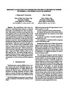
example, in the ISM band, Bluetooth Wireless Personal Area Network (WPAN) coexist with the IEEE802.11 Wireless Local Area Network (WLAN), cordless phones, radio frequency identification (RFID) cards and microwave ovens. As a result, there has been a growing interest of increasing spectral efficiency by shifting from “exclusive spectrum usage rights policy” to “shared spectrum policy”. Several recent measurements of spectrum usage indicate that many licensed spectrum bands remain relatively unused for most of the time [1, 2, 3, 4]. The measurements taken by Berkeley Wireless Research Center show that the allocated spectrum is vastly underutilized [1]. Measured results of spectrum usage activity (green means no activity) in downtown Berkeley, California are shown in Fig. 1.1. It has been reported in [2] that utilization in 30-300 MHz spectrum band is only 5.2%. In [3], it has been reported that utilization of spectrum below 3 GHz can be as low as 15%. The rest 85% of the time, unused spectrum can be allocated to “secondary users”- users without a license to operate in the band. Spectrum sharing has shown to increase spectrum utilization and has been proven to be successful and commercially practical. Allowing secondary users to operate with minimal or no interference to primary users is one way of spectrum sharing. Therefore, FCC has opened up licensed bands for opportunistic use by secondary users since 2004 [5]. In order to enable secondary users to coexist with other users in a frequency band, the radio receiver must be opportunistic [6]. Opportunistic users must quickly identify and exploit available frequency bands/channels. They must also be willing to be ready to be interrupted and look for other channels to complete transmission. This concept is called Dynamic Spectrum Access (DSA). DSA requires the radio to have the following features: (i) Intelligence: the radio must sense the environment and identify spatial, temporal or spectral voids. (ii) Programmable: the radio must be programmable to change transmission parameters such as power level, modulation order, operating frequency, transmission bandwidth, coding rate, frame size to achieve certain performance goals/QoS objectives. (iii) Agility: the radio must be able to hop quickly to available channels. (iv) Broadband: the radio must
2
Figure 1.1: Measurements of spectral usage activity in downtown, Berkeley ([1]).
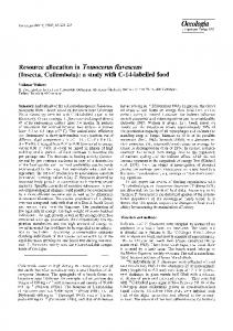
be able to scan a large number of channels in order to increase the probability of correctly identifying free channels to avoid long interruption in transmission. (v) Low cost: the cost of the radio has to be comparable with current technology. (vi) Low power consumption: power consumption of the radio has to be comparable with current wireless devices. A cognitive radio (CR) has been considered as a possible enabling solution for a DSA system. The concept of cognitive radios was first introduced by Joseph Mitola III [7]. Joseph Mitola III defines cognitive radio as an extension of software defined radio (SDR) that employs model-based reasoning about users, multimedia content and communication context. The cognition cycle employed in investigated cognitive radio architectures at Royal Institute of Technology (KTH) is shown in Fig. 1.2. In [7], cognitive radio is defined as a goal-driven framework in which the radio senses the environment, infers context, assesses alternatives, generates plans, supervises multimedia services and learns from its mistakes. As a DSA compatible system, cognitive radio adapts to the environment by sensing the spectrum and takes quick decision on appropriate transmission parameters to achieve certain 3
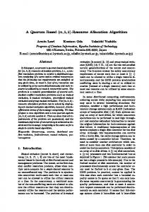
performance goals. A cognitive radio can be envisioned as shown in Fig. 1.3 [8]. Figure 1.3 depicts how the environmental parameters (as dials) and transmission parameters (as knobs) interact and are used in a cognitive radio. Orient Infer on context hierarchy
Establish priority
Pre-process
Normal Immediate
Urgent
Parse
Plan
Observe
Learn Register to current time
New States Save global states
Prior States
Receive a Message Read Buttons
Generate and Evaluate Alternatives
Send a message
Decide Allocate resources
Act
Initiate processes
Set display
Outside World
Figure 1.2: Cognition cycle ([7]).
A cognitive radio network (CRN) is defined as a network of cognitive radios/secondary users. The first task that a secondary user (SU) in CRN needs to perform is sensing the activity of primary users in its intended channel/channels. All SUs in CRNs maintain QoS through the transmission duration by dynamically seeking out the best transmission strategies (e.g., channel, rate, transmit power). In the following section, we introduce some of the challenges in CRNs and describe related prior work.
1.2
Challenges in CRNs and Prior Work
The challenges in CRNs can be broadly listed as 1. Cognitive radio architecture and implementation issues [6]-[12],
4
Figure 1.3: Visual representation of cognitive radio dials and knobs ([8]).
2. Spectrum sensing hardware requirements [6]-[11], 3. Spectrum sensing algorithms [13]-[29], 4. Resource management [30]-[53], 5. Fairness in resource allocation [54]-[66], 6. Policy challenges [67]-[71]. In this dissertation, we are primarily focused on addressing challenges in resource management and fairness which are implicitly related to spectrum sensing algorithms. Therefore, we present an overview of prior work in those areas in the following subsections.
1.2.1
Spectrum Sensing
Spectrum sensing is the most important and first task for a SU in CRNs. Spectrum sensing technique in CRNs has been widely studied. The sensing function requires the radio to step through a set of frequency bands and perform signal detection for each frequency band. Different sensing techniques such as matched filter, energy detector and cyclostationary 5
feature detection have been reviewed in [13]. Matched filtering [13] is the optimum method for detection of primary user (PU). Effectively, a matched filter does the demodulation of a PU signal. Hence, in matched filtering approach, SU is required to have priori knowledge of PU signal (such as modulation type, modulation order, pulse shaping, packet format). That is, a SU needs a dedicated receiver for every primary user class, which makes matched filtering approach impractical in CRNs. Energy detector [13] detects the signal by comparing the output of energy detector to a preset threshold and does not require any information of PU signal. Threshold setting requirement makes the energy detector vulnerable to noise and interference level. Cyclostationary feature detection approach [13] is based on properties of the modulated signal. Modulated signals are in general coupled with sine wave carriers, pulse trains or cyclic prefixes which result in built in periodicity. This periodicity helps to extract the information such as modulation, pulse shape of the received signal. In cyclostationary feature detection, instead of power spectral density, cyclic correlation function is used for detecting the signals present in the spectrum. A modified version of cyclostationary feature detector to improve spectrum sensing performance at low signal to noise ratio (SNR) is proposed in [14]. The modified detector in [14] performs the autocorrelation of received signal before the spectral correlation detection. The authors in [15] propose a sensing method to identify PU by estimating their radio frequency (RF) transmission parameters. The identification is done by matching the a priori information about PU transmission parameters to the features extracted from the received signal. In [16], the authors show a PU detection technique exploiting the local oscillator (LO) leakage power emitted by the RF front end of primary receivers. The authors in [18] derive a blind sensing algorithm based on oversampling the received signal or by employing multiple receive antennas. The proposed method in [18] does not require any information of PU signal or channel. The proposed method combines linear prediction and QR decomposition of the received signal matrix. Two signal statistics are computed from the oversampled received signal. The ratio of these two statistics indicates the presence/absence of the PU signal.
6
To increase spectrum sensing performance, network based sensing [24], cooperative sensing [25, 27, 28] have been proposed. The techniques in [24, 25, 27, 28] increase sensing time and are not well suited for practical implementation of cognitive radio in time sensitive operations. The authors in [29] propose the use of dedicated sensing receiver (DSR) that solely focuses on channel sensing and runs in parallel with a main receiver. Here, the authors also show that the DSR architecture provides up to a fivefold reduction in total mean detection time.
1.2.2
Resource Allocation
After the spectrum sensing phase, each SU in a CRN needs to identify its operating channel/channels, transmit power level, modulation type, modulation order, channel coding, spectral shaping etc. There have been significant research efforts related to determining optimal channel, transmit power, modulation type and rate for SUs [30, 31, 32, 33, 34, 35, 36, 8, 37, 38, 52, 53]. The authors in [30, 31] consider a CRN model with one PU and one SU coexisting in the same channel. In [30], power allocation strategies for the SU are developed with the objective of maximizing ergodic capacity under different constraints (such as limits on peak and average transmit and interference power). In [31], the authors develop a cognitive radio game to find optimal transmit power with the goal of minimizing total transmit power. Here, quality of service (QoS) is maintained for the PU (defined as minimum rate and maximum acceptable bit error rate (BER)). The authors claim that their formulation is applicable to the case when multiple SUs share a channel. In [32, 33], the authors consider a CRN model with one PU and multiple SUs coexisting in the same channel. Here, the authors develop distributed power allocation strategies for the SUs. The authors in [34, 35, 36] consider a system model where multiple SUs coexist in a channel. In [34], the authors design a power control game with a utility function of maximizing transmission rate to find transmit power. In [35], the authors study both centralized and distributed auction mechanisms to
7
allocate receive powers. They consider an objective function of maximizing utility which is a function of signal to interference plus noise ratio (SINR). The authors in [36] design a convex optimization problem to find optimal transmit power. A lower bound on SINR is used as a QoS constraint for secondary users. A distributed suboptimal joint coordination and power control mechanism to allocate transmit powers to secondary users is also presented in [36]. A genetic algorithm driven cognitive radio decision engine is employed to determine the optimal transmission parameters (transmit power, modulation type and rate (modulation order)) for a SU in both single and multi-carrier based CRNs in [8]. The approach presented in [8] suffers from numerous drawbacks. Genetic algorithms are notorious for slow convergence and high complexity. Therefore, their implementation is not suitable for time varying environments as well as delay sensitive applications. Additionally, the underlying optimization problem in [8] has non-convex fitness function which in turn implies that the optimality of the genetic algorithm based solution cannot be guaranteed. In [37, 38], joint allocation of channel and transmit power for multi-channel multiuser CRN has been studied. The authors in [38] apply game theory to develop distributed power allocation algorithm. However, in [37], coexistence of multiple secondary users in a channel has not been considered. Also, in [37, 38], the QoS requirement of SUs has been ignored. In [72], the authors propose two game theoretic approaches using potential game framework and ϕ-no-regret-learning schemes to allocate available channels to secondary users. Both approaches show better performance compared to random channel allocation. In [52], the authors propose a stochastic channel selection based on learning automata technique to maximize the probability of successful transmissions and to avoid frequent channel switchings in CRN. A biologically-inspired spectrum sharing algorithm based on the adaptive task allocation model in insect colonies to select channel has been presented in [53]. However, in [52, 53], though the authors have considered multiple channels to start with, only one secondary user is eventually assigned a channel.
8
1.2.3
Fairness in Resource Allocation
When multiple SUs compete for a limited number of available channels/frequency bands in CRNs, fairness among SUs in resource allocation is another important consideration. Fairness issues in resource allocation has garnered some attention in recent years [54, 55, 56, 57, 58, 66]. The authors in [54] focus on deriving fair (in terms of airtime share) random access protocol for dissimilar radio systems in open spectrum access scenario. In their proposed fair random access protocol, each radio system contends for the spectrum with a finite probability. The authors also propose a Homo Egualis (HE) society model based distributed approach to determine the contending probability. In [55], the authors propose a fair opportunistic spectrum access using fast catch-up strategy that reduces the first passage time (first passage time is the amount of time after which all SUs have equal access right to the available channels). In [56], the authors study three variants of utility functions to allocate spectrum in CRN under protocol interference model. The variants are Max-sum-Reward, Max-min-Reward and Max-Proportional Fair utility functions. The authors map the different spectrum allocation problems into color-sensitive graph coloring (CSGC) problem and consider binary geometry interference model. As the optimal graph coloring problem is NP-hard, the authors also present heuristic to solve the allocation problems. In [57], the authors study the joint spectrum allocation and scheduling in CRN with the objective to achieve a tradeoff between throughput and fairness while ensuring interference-free transmission at any time (taking into account both protocol and physical interference models). The authors in [57] transform the joint allocation and scheduling problem into a problem of finding all possible transmission modes and the active time fraction for each transmission mode. A transmission mode is composed of a subset of user-channel pairs which can be active concurrently. They define three joint spectrum allocation and scheduling problems and these are MAximum throughput Spectrum allocation and Scheduling (MASS), Max-min fair MAximum throughput Spectrum allocation and Scheduling (MMASS) and Proportional 9
fAir Spectrum allocation and Scheduling (PASS). The MASS problem finds a feasible rate allocation vector, all transmission modes along with a feasible transmission schedule vector such that the throughput is maximized. To avoid starvation of some users due to maximizing throughput, the authors consider a new variable called Demand Satisfaction Factor (DSF) into the scheduling problem. The DSF of a user is defined as the ratio of rate allocated to that user over its traffic demand. In MMASS, the rate that minimizes the maximum dissatisfaction with respect to demand is evaluated. The PASS problem finds a feasible rate allocation vector, all transmission modes along with a feasible transmission schedule vector such that the summation of the logarithmic of DSF is maximized. The authors in [57] also conclude that PASS formulation provide a better tradeoff between throughput and fairness compared to MASS or MMASS. The authors in [58] develop a set of resource allocation exploiting fairness axioms of game theory that provides fairness in allocating the “extra” resources available after satisfying the minimum requirements of primary users. In [66], the authors find optimal transmit power for users in wireless cellular and ad hoc networks considering proportional and minmax fairness. In proportional fairness resource allocation scheme formulation, the authors consider a static weight for each user and use the weight into resource allocation scheme. In minmax fairness resource allocation scheme formulation, the transmit power that maximizes the minimum signal to interference ratio is determined.
1.3
Motivation and Overview
We believe that in a practical CRN, (1) multiple channels may be available, and (2) multiple SUs may compete for available resources. To increase spectral efficiency, multiple SUs may coexist in a channel. Also, channels may be of different quality. Therefore, the SUs assigned to higher quality channels may hold an advantage over SUs assigned to the poorer channels and rate requirement of some secondary users may not be satisfied by allocating one channel to a user. That is, in practice, a single SU may occupy more than one channel.
10
Resource management in such a practical CRN is an important consideration that has not yet been addressed. The primary research question we answer in this dissertation is: How can we optimize transmit power and rate (modulation order) in a competitive CRN while maintaining QoS for SUs? Before we answer this question, the “coexistence of multiple SUs in a channel” motivates our first task in this dissertation. In a competitive environment where multiple SUs coexist in a single channel, one can expect the QoS of one user to depend on the number and behavior of other SUs. Much of the prior work in CRNs has primarily been focused on sensing primary users with very little emphasis on how multiple secondary users may compete for available spectrum. Therefore, forecasting the behavior of secondary users is equally critical in the successful operation of a CRN. For example, if a spectrum band is determined to be free and a large number of secondary users decide to use this spectrum band simultaneously, the QoS or BER performance of the secondary users will degrade due to high level of interference. Therefore, it is important to investigate strategies for enabling SUs to sense and predict the behavior of both primary and competing secondary users in a frequency band of interest. In this context, firstly we are motivated to introduce an integrated modeling and forecasting framework for monitoring spectrum use by primary and secondary users in CRNs. Next, we assume scheduling is complete and SUs have identified the channels to use. Now, our goal is to determine the optimal transmit power and rate (modulation order) that competing SUs need to employ in each channel. In this context, we propose two resource allocation frameworks. In both frameworks, our objective is to determine the optimal distribution of power and rate that a secondary user has to employ across the channels that it uses in order to (1) minimize total power consumption; (2) maximize rate, and (3) maintain QoS. Our measures for QoS include SINR or BER and minimum rate requirement. The proposed resource allocation frameworks provide the optimal transmit power and rate across the channels for all SUs for a given time instant. However, users may not be
11
satisfied with optimal allocation of resources based on instantaneous QoS. An example of dissatisfaction among SUs may arise when two SUs with different minimum rate requirements are allocated the same rate. Another example of dissatisfaction among SUs may arise when a user expends higher power relative to other users. Typically dissatisfaction is a feeling that develops over time. Hence, unlike prior efforts in resource allocation, it is imperative to consider user experience over time. Subsequently, the question that needs to be addressed is “Can we maintain fairness in user experiences over time?” To answer this question, we borrow ideas from social behavioral models and apply it to the resource management solutions in a competitive CRN setting. The centralized solution of the proposed resource allocation frameworks demand extensive control signalling and is difficult to implement in practice if information exchange about all users and channels is limited. In this context, we are motivated to develop distributed user-based approaches to solve the proposed resource allocation frameworks.
1.4
Contributions
We consider a CRN with multiple channels available for opportunistic use by multiple SUs. We also assume that multiple SUs may coexist in a channel and each SU can use multiple channels to satisfy their rate requirements. The CRN operation is shown in Fig. 1.4. Figure 1.4 tells that each SU scans the spectrum at regular intervals and starts transmitting on particular channel/channels once it determines that the channel/channels will not be used by a PU. At any instant of time, SUs ceases transmission through channel/channels if PU enters in that particular channel/channels. The key contributions of this dissertation for such a CRN setting are summarized in this section. 1. Assuming that the spectrum usage of various channels are independent, for the first time we present an integrated modeling and forecasting framework for monitoring spectrum use by primary and secondary users in a competitive CRN. (a) Assuming a continuous time Markov chain model for both primary and secondary 12
time t1
Ch-1
Ch-2
Ch-k
PU arrives
…
Ch-L
SU leaves
time (t1 + Tm )
Ch-1
Ch-2
Ch-k
…
Ch-L
time (t1 + 2Tm )
Ch-1
Ch-2
Ch-k
…
Ch-L
- Available channels/PU in use - Available channels/1 or more SU in use
Figure 1.4: CRN operation (Tm denotes measurement interval).
users activities, we propose a Kalman Filter based approach for estimating the number of primary and secondary users. These estimates are in turn used to predict the number of primary and secondary users in a future time instant. (b) Using both simulated data and measured power levels in the 2.4 GHz unlicensed band, we demonstrate the implementation of both the modeling and forecasting aspects of the proposed approach. We observe that our proposed forecasting technique, not only provides a good upper bound prediction for the number of primary and secondary user, it is also robust to model parameter estimation errors. (c) We extend the modeling and forecasting framework to the case when SU traffic is governed by Erlangian process, (i.e., the traffic model incorporates bulk arrival or bulk departure scenarios). (d) Knowledge of the upper bound provides valuable information to a SU interested in using a spectrum band that is already being used by other secondary users. Detailed analysis of proposed modeling and forecasting tools are provided in chapter 2 and in our papers [73, 74, 75]. 2. We propose two centralized resource allocation frameworks for resource allocation to secondary users in a competitive CRN. 13
(a) In the first framework, we propose a two-stage process. In the first stage, optimal choice for transmit power is determined for all SUs subject to maintaining a given SINR in each channel used. Using this power/SINR result, the optimal distribution of rate (modulation order) is determined in the second stage. In the second stage, the rate distribution is formulated as a maximum flow problem in graph theory. We also propose a simple heuristic to determine the rate allocation. (b) In the second framework, we jointly determine the best choice of power and rate distribution for every SU with the help of a bi-objective problem formulation. (c) Unlike prior efforts, we have transformed the BER constraint in both frameworks into a convex constraint in order to ensure optimality of our resulting solutions. (d) In both frameworks, we observe that optimal transmit power follows reverse water filling process and optimal rate allocation is proportional to SINR. (e) In terms of total power (i.e., net transmission cost), the joint optimization framework is more economical relative to the two-stage optimization framework. This is because, the joint formulation offers more degrees of freedom with the ability to adapt both power and rate simultaneously in order to achieve a certain BER. In the two-stage optimization framework, either power or rate is available to adapt to achieve a certain SINR or BER, respectively. Detailed analysis of the proposed resource allocation frameworks are provided in chapters 3, 4 and in our paper [76]. 3. In a competitive CRN, for the first time we determine optimal power and rate distribution choices for each SU while maintaining fairness in current and prior history of user experience with respect to QoS among SUs. (a) We quantify user experience over time by introducing dynamic fairness weights for each SU in the resource allocation framework. (b) The dynamics of the weights are governed by social behavioral models. We study 14
the effect of Homo Egualis (HE), Homo Parochius (HP) and Homo Reciprocan (HR) models. (c) We observe that considering dynamic fairness weights in the resource allocation scheme provide a better system level fairness index (as defined by Jain in [77]) relative to the unweighted allocation scheme. Detailed analysis of the proposed resource allocation framework is provided in chapter 5 and in our papers [78, 79]. 4. With the help of dual decomposition theory [80], we develop three (3) user-based distributed approaches to solve the resource allocation framework introduced in 2. We observe that the solution from each distributed implementation for both frameworks follows the centralized solution. Detailed analysis of the proposed distributed algorithms are provided in chapters 3, 4 and in our papers [81, 82]. 5. Finally, we develop game theory based implementation for joint resource allocation framework. We analyze existence of Nash Equilibrium for the game. We develop an algorithm to reach Nash Equilibrium. Detailed analysis of the proposed distributed algorithm is provided in chapter 6 and in our paper [83].
1.5
Organization
The dissertation is organized into seven chapters. Chapter 2 presents the modeling and forecasting tool for secondary users activity. We develop estimation and forecasting tools for both Poissonian and Erlangian traffic model activities of secondary users. Numerical results on predictor performances for both traffic cases are also provided. In chapter 3, we introduce the two-stage resource allocation framework. We present dual based distributed approaches to solve stage 1. Optimal and heuristic rate distribution for stage 2 are provided. Additionally, a comparison on centralized and distributed power allocation, and optimal and heuristic rate allocation are shown. Chapter 4 contains the joint resource allocation framework along with its dual distributed implementations. Besides, a comparison on resource 15
allocation between two-stage and joint allocation schemes as well as between centralized and distributed joint allocation schemes are provided. In chapter 5, we describe the resource allocation framework incorporating dynamic fairness weights. We present the analogy between the social behavior of human beings and that of SUs in CRN, and the society models of interest to this work. Chapter 6 shows the game theoretic implementation of joint resource allocation framework. Here, we analyze the existence of the Nash Equilibrium. We develop an algorithm to reach the NE. Finally, chapter 7 concludes the dissertation and possible future directions and extensions of this work.
16
Chapter 2 Spectrum Usage Modeling and Forecasting In this chapter, we seek a solution for the first task in chapter 1. Specifically, we introduce an integrated modeling and forecasting approach that SUs in a CRN can use to predict spectrum usage/availability based primarily on power level measurements. Our modeling and forecasting setup incorporates traffic behavior of both primary and competing secondary users in a spectrum band of interest. Firstly, by considering a continuous time Markov chain traffic model for PU and SUs, we propose a Kalman filter approach to estimate the number of primary and secondary users at a given time instant. Based on these estimates, we determine robust upper bound forecasts of the number of primary and secondary users for a future time instant. Secondly, we generalize the SU traffic model and develop estimation and forecasting tool accordingly. It is important to remember that this chapter offers a modeling and forecasting tool and not algorithms for spectrum sharing among multiple secondary users. Additionally, note that even though we use the words spectrum band, frequency band and channel interchangeably throughout the chapter, they convey the same meaning. The rest of the chapter is organized as follows. In Sec. 2.1, we describe the proposed spectrum usage model in detail for Poissonian traffic model. Section 2.2 presents the Kalman filtering techniques to estimate the number of primary and secondary users and Sec. 2.3
17
describes the proposed forecasting techniques for both primary and secondary users. Experimental results illustrating the application of the modeling and forecasting methods are provided in Sec. 2.4. Section 2.5 develops the estimation and prediction tool for SU generalized traffic model and also presents the performance of the predictors. Finally, conclusions are presented in Sec. 2.6.
2.1
System Model
We consider L channels within a CRN as shown in Fig. 1.4. Each of the L channels can be used by either a PU or one or more secondary users. Each SU uses the spectrum opportunistically. That is, every SU scans the spectrum at regular intervals and starts transmitting on a particular channel once it determines that the channel will not be used by a PU. Typically, researchers focus on the sensing aspect of secondary users in order to determine if a channel is available for transmission. In this chapter, in addition to determining the presence or absence of the primary user in a given channel, we also consider the impact of multiple secondary users utilizing a single channel. For example, if a channel is determined to be free and a large number of secondary users decide to use this channel simultaneously, the QoS (SINR or BER) performance of the secondary users will be poor due to high level of interference from other secondary users. Consequently, it is important for every SU to monitor the spectrum usage by other secondary users and this aspect is captured in our proposed modeling and forecasting set up. Additionally, we assume that the spectrum usage of various channels are independent. Therefore, in the rest of the chapter, we restrict ourselves to the modeling and forecasting of spectrum use to one channel. It is easy to extend the idea presented in the following sections to the case of correlated channels. We assume that both the PU and secondary users follow Poisson arrival process with rates, λp and λs , respectively. Their negative exponential service time distributions have rates, µp and µs , respectively. A similar model for arrival and departure processes of PU 18
and secondary users have been assumed in [54, 84]. The maximum number of PU and SU are Np and Ns , respectively. For ease in presentation, Np is assumed to be equal to 1, i.e., we assume that PU is either present or absent. In other words, PU follows a two-state ON-OFF Markov process. The two-dimensional state-transition-rate diagram for the CRN is shown in Fig. 2.1. λp 0, 0
µs
1, 0
N s λs
µp ( N s − K )λ s
( N s − 1)λs
0, 1
0, 2
…
0, K
0, K + 1 …
( K + 1) µ s
2µ s
λs
0, Ns − 1
0, Ns
Ns µs
Figure 2.1: Two-dimensional state-transition-rate diagram of PU and SU.
Each state in the model is denoted as (np , ns ), where np and ns represent the number of primary user and secondary users, respectively. From this state-transition-rate diagram and concepts from queueing theory [85], the differential equations for the state probabilities, pri,k (t) can be evaluated for both primary (with i = p) and secondary (with i = s) users. The state probability is defined as pri,k (t) , prob{xi (t) = k},
(2.1)
where, xi (t) is the number of users at time t and k indicates that number. Since we have an ON-OFF traffic model for PU, k = 0 or 1 when i = p. On the other hand, for secondary users, i.e., when i = s, k can vary from 0 to Ns provided that there is no primary user in
19
the channel. In general, the differential equations for the state probabilities correspond to d pri,0 (t) = µi pri,1 (t) − Ni λi pri,0 (t), dt ·
(2.2)
· · d pri,k (t) = (Ni − k + 1)λi pri,(k−1) (t) + (k + 1)µi pri,(k+1) (t) dt −(kµi + (Ni − k)λi )pri,k (t), 1 ≤ k < Ni ,
(2.3)
· · · d pri,Ni (t) = λpri,(Ni −1) (t) − Ni µi pri,Ni (t), for i = p, s. dt
(2.4)
Typically, we are interested in determining the expected number of primary and secondary users in a given time instant. Therefore, the E{xi (t)} can be written as E{xi (t)} =
Ni ∑
kpri,k (t), for i = p, s.
(2.5)
k=0
Hence, i ∑ d d k pri,k (t), for i = p, s. E{xi (t)} = dt dt k=0
N
(2.6)
Let LQ = [0 1 2 · · · Ni ]T . From Eqs. (2.2)-(2.4), (2.6), we can write d E{xi (t)} = LTQ P˙ i = LTQ Qi Pi , dt
(2.7)
where, Qi =
−Ni λi µi 0 · 0 Ni λi −[(Ni − 1)λi + µi ] 2µi · 0 0 (Ni − 1)λi −[(Ni − 2)λi + 2µi ] · 0 0 · · · 0 0 0 · λi −Ni µi 20
and
Pi =
pri,0 (t) pri,1 (t) · · · pri,Ni (t)
, for i = p, s.
In Eq. (2.7), (·)T indicates matrix or vector transpose operator. LTQ Qi Pi is obtained as Ni λi − (λi + µi )E{xi (t)}. Therefore, d E{xi (t)} = Ni λi − (λi + µi )E{xi (t)}. dt
(2.8)
We assume that measurements are performed at discrete time instants mTm , m = 1, 2, 3, · · · for a given value Tm . Using the initial condition that the number of users at time t = (m − 1)Tm is xi (m − 1), the solution of Eq. (2.8) is obtained as E [xi (m)|xi (m − 1)] = xi (m − 1)e−Tm (λi +µi ) +
] Ni λi [ 1 − e−Tm (λi +µi ) . (λi + µi )
(2.9)
Therefore, it is possible to express the number of users (primary or secondary) at time mTm in terms of the number of users (primary or secondary) at time (m − 1)Tm as xi (m) = Ai xi (m − 1) + Bi ,
(2.10)
Ai = e−Tm (λi +µi )
(2.11)
where,
and Bi =
] Ni λi [ 1 − e−Tm (λi +µi ) . (λi + µi )
(2.12)
Equation (2.10) shows us the relationship between the number of users at two successive measurement instants and in most general case, Eq. (2.10) corresponds to xi (m) = Ai xi (m − 1) + Bi ui (m) + wi (m), for i = p, s. 21
(2.13)
Specifically, we can write down the state equations for primary and secondary users as xp (m) = Ap xp (m − 1) + Bp up (m) + wp (m)
(2.14)
xs (m) = As xs (m − 1) + Bs us (m) + ws (m),
(2.15)
and
where, xp (m) and xs (m) represent the number of primary and secondary users using the spectrum, respectively, at the measurement instant m. The parameters Bp and Bs relate the optional control inputs up (m) and us (m), respectively to states. Equation (2.10) suggests that up (m) and us (m) are equal to 1 for our system model. wp (m) and ws (m) are the process noise and assumed to be zero mean Gaussian noise with variances σp2 and σs2 , respectively. The parameters Ap and As relate the states at previous and current measurement instants, in the absence of either a driving function or process noise. Ap and As are assumed to be constant over the analysis or vary very slowly. The received power at a secondary user terminal during the measurement instant m consists of relative power level increments caused by both primary and secondary users and in the most general case corresponds to, y(m) = Cp xp (m) + Cs xs (m) + D + v(m),
(2.16)
where, y(m) is received power in dBm; Cp and Cs represent the relative increase in power level (in dB) due to the presence of primary and secondary users, respectively; D represents the background thermal noise and v(m) denotes the measurement noise which may arise due to miscalculation, misalignment of timings and is assumed to be zero mean Gaussian noise with variance σv2 . y(m) is the only measurable variable in the system. In a CRN, the primary user has the right of use. Therefore, modeling and forecasting tasks are more critical for secondary users. From a secondary user perspective, we assume two modes of operation. Once a SU decides to use a channel opportunistically, it will enter a “learning and modeling phase.” In this phase, the SU measures the power levels in the 22
channel and estimates traffic parameters of primary and other secondary users. An example of this estimation process is discussed in Sec. 2.4 where a time series based approach is used for modeling. In the next phase, the SU becomes an “active” participant in opportunistic spectrum sharing process. In the “active” phase, each secondary user continues to sense the received power level in order to forecast the use of spectrum by other secondary users. This process is illustrated in Fig. 2.2. Ch-1
Ch-2
…
Ch-k
…
…
Ch-L
Power level of Ch-k is measured at current measurement instant
Estimate the no. of PU Forecast the no. of PU for next measurement instant
SU (if any is still transmitting) ceases
1 PU = 1or 0
0 Estimate the no. of SU Forecast the no. of SU for next measurement instant
Figure 2.2: Operation of the system on a single channel’s spectrum usage in “active phase.”
23
2.2
Estimation of Spectrum Usage
In Sec. 2.1, we introduced the traffic models for the number of primary and secondary users using a given channel. In this section, we propose a Kalman filter based state estimation technique (i.e., estimating the number of primary and secondary users) based on the model from Sec. 2.1. The state estimation based on Kalman filter is summarized below: State Equation: The state of the CRN can be represented by a vector x = [xp xs ]T . The corresponding state equation is x(m) = Ax(m − 1) + B + w(m), where,
[ A=
Ap 0 0 As
[
] ,B=
Bp Bs
(2.17)
]
and w(m) is a vector white Gaussian noise with mean 0 and covariance matrix, [ 2 ] σp 0 Σw = . 0 σs2 Measurement Equation: y(m) = CT x(m) + D + v(m),
(2.18)
where CT = [Cp Cs ]. Based on the state and measurement equations Eqs. (2.17) and (2.18), respectively, the Kalman filtering steps are given below: Step 1: Initialization [ b(0|0) = x
E(xp (0)) E(xs (0))
]
[ and M(0|0) =
σp2 (0) 0 2 0 σs (0)
] .
(2.19)
Step 2: Prediction b(m|m − 1) = Ab x x(m − 1|m − 1) + B, ∀ m M(m|m − 1) = AM(m − 1|m − 1)AT + Σw , ∀ m
(2.20) (2.21)
Step 3: Kalman gain vector calculation ( )−1 K(m) = M(m|m − 1)C CT M(m|m − 1)C + σv2 ,∀m 24
(2.22)
Step 4: Correction ( ) b(m|m) = x b(m|m − 1) + K(m) y(m) − CT x b(m|m − 1) − D , ∀ m x M(m|m) = {I − K(m)CT }M(m|m − 1), ∀ m
(2.23) (2.24)
From Eqs. (2.19)-(2.24), we estimate the number of primary and secondary users. The estimated value for the number of secondary users denoted as x bs (m|m) is reset to 0 if the predicted value for the number of primary user for (m + 1) th instant is 1. This is also depicted in the block diagram in Fig. 2.2. The prediction methods for both primary and secondary users is described in the following section.
2.3
Forecasting Spectrum Usage
In this section, we describe the forecasting techniques used to predict the activity of primary and secondary users in the channel of interest. One approach for forecasting is to determine the likely state at the next time instant given that we have the state estimate for the current instant. For this, we need to calculate the probability of transitioning to another state at time (m + 1)Tm . The transitioning probabilities can be determined starting from the following differential equation, ˙ i = Qi Pi , for i = p, s P
(2.25)
within the time interval mTm < t < (m + 1)Tm . The Pi and Qi are as defined in Sec. 2.1. Equation (2.25) governs the evolution of state transition probabilities. The solution of Eq. (2.25) gives the state transition probabilities from the m th measurement instant. The existence of the solution of Eq. (2.25) depends on two conditions. The first condition is the diagonalizable property of matrix Qi . The second one is non-positive definiteness of matrix Qi . The matrix Qi satisfies both conditions. It is reducible to a diagonal form Qi = Ei Γi E−1 i , where Γi is a diagonal matrix with eigenvalues of Qi , and Ei is the matrix of corresponding right eigenvectors. The eigenvalues can be found to be γr = −r(λi + µi ) 25
for r = 0, · · · , Ni . Hence, the solution, for t ∈ (mTm , (m + 1)Tm ], is given by Pi = Ei eΓi t Fi , for i = p, s;
(2.26)
where Fi is a constant vector determined from the initial condition (i.e, x bi (m|m)) as Fi = (eΓi mTm )−1 E−1 i PmTm (i) ,
(2.27)
where PmTm (i) is a vector with all 0’s except the x bi (m|m)) th element which is 1. Now, we compute state transitioning probability values for the instant (m + 1)Tm by integrating the time varying state transitioning probability expressions (i.e., Eq. (2.26)) [86] as ∫ (m+1)Tm 1 ei = P Pi dt Tm mTm (∫ ) (m+1)Tm 1 = Ei eΓi t dt Fi Tm mTm =
1 [pr e pr e · · · pr e i,Ni ]T , for i = p, s. Tm i,0 i,1
(2.28)
In the above integration notation, we have used the fact that the integral of a matrix is e i denote the the integral of each element of the matrix. The elements pr e i,k of the vector P probabilities of transitioning to state k at instant (m+1)Tm , for i = p, s. Based on the state transitioning probabilities, we can now forecast the number of primary and secondary users. For ease in presentation, the forecasting method for spectrum usage of SU is described first.
2.3.1
Forecasting Spectrum Usage of SU
Forecasting spectrum usage by other secondary users is critical for the following reasons. Each SU can now determine if a particular channel is overcrowded with secondary users. If it is, the channel may be avoided as it may degrade the QoS. Additionally, by forecasting the number of secondary users in a channel, each SU can also determine how much power it needs to transmit without violating spectral emission limits (while maintaining its QoS). In this dissertation, we propose an upper bound forecasting based on state transitioning probability matrix of SU similar to the approach taken for forecasting the number of flows in 26
Internet traffic [86]. We discuss the case when the number of PU is 0 and we are interested in forecasting the number of secondary users at the next instant. The optimal estimate of the number of secondary users i.e., x bs (m|m), at time instant m is used to forecast the number of secondary users at (m + 1) th instant. Based on estimated number of secondary users, x bs (m|m) at time mTm , state transitioning probability values is computed from Eq. (2.28) and then prediction for (m + 1) th instant is done. The predicted state of SU for (m + 1) th instant at time mTm corresponds to [86], x es (m) =
min
xs ∈[b xs (m|m), Ns ]
xs s.t. pr e s,k < β.
(2.29)
Here, β is pre-set probability value. Equation (2.29) can be understood with the help of an example. Suppose, x bs (m|m) is obtained as 3 and Ns is 8. Based on the value of x bs (m|m), es = a state transition probability vector i.e., P
1 [pr e s,0 Tm
pr e s,1 · · · pr e s,8 ]T is obtained, which
corresponds to the possible states of SU with number of users [0 1 · · · 8]T , respectively. By observing this state transition probability vector, one can determine multiple states for which pr e s,k < β. All states with number of users greater than 5 might satisfy this condition. This effectively suggests that the probability of xs (m + 1) being 5 or more is going to be negligible. Therefore, the upper bound for the xs (m + 1) should be 5. In general, the chosen state is the state with minimum number of user satisfying Eq. (2.29). As a result, Eq. (2.29) serves as a good upper bound for the number of secondary users at time (m + 1) based on measurements up to time m.
2.3.2
Forecasting Spectrum Usage of PU
We propose two ways to forecast the presence or absence of a primary user. The first method is Kalman filter (KF) based prediction. In this method, the number of primary user obtained from the prediction stage (Eq. (2.20)) is used as the forecasted number of primary user. For example, from the estimated value at m th instant, x bp (m|m), the predicted value
27
for (m + 1) th instant at m th instant is taken as, ep (m) = x bp (m + 1|m) x = Ap x bp (m|m) + Bp .
(2.30)
The second method is based on state transitioning probabilities as given in Eq. (2.28). In this method, state transition probabilities from the present estimated state x bp (m|m) is computed in the same way as it is described for SU above and state with higher state transition probability is taken as predicted state x ep (m). For the proposed system model in this chapter, Markov chain of PU shows that it follows two states - state 0 (number of PU is 0) and state 1 (number of PU is 1). Suppose, x bp (m|m) is obtained as 1 and based on this, ep = a state transition probability vector i.e., P
1 [pr e p,0 Tm
pr e p,1 ]T is computed. The predicted
state of PU for (m + 1) th instant at time mTm is proposed as, { 1, if pr e p,1 > pr e p,0 , x ep (m) = . 0, otherwise
2.4
(2.31)
Experimental Results
In this section, we illustrate the potency of the proposed techniques for estimating and forecasting spectrum usage in a cognitive radio network through simulation. We show the performance of proposed methods on two different sets of data - (1) simulated data from a CRN; (2) real time measurement data from 2.4 GHz ISM band.
2.4.1
Simulated CRN
We consider a CRN where PU follows an ON-OFF Markov process with arrival rate (λp ) and departure rate (µp ), 0.000625 sec−1 and 0.00125 sec−1 , respectively. For primary user, λp is set smaller compared to µp to reflect the assumption that the primary user arrives less frequently but once it comes, it stays longer. The above choices for λp and µp reflect a 32% use of the channel by the PU on average. We assume that a SU is in “active phase,” i.e., SU knows all required traffic parameters. In our set up, secondary users follow Markov process 28
with 11 states. The arrival rate (λs ) and departure rate (µs ) are taken as, 0.005 sec−1 and 0.005 sec−1 , respectively. The state noise variances, σp2 and σs2 are considered as 0.2 and 1, respectively. These parameters are summarized in Table 2.1. Table 2.1: Statistics of primary and secondary users. Primary User Np = 1 Cp =30 σp2 =0.2 λp =0.000625 µp =0.00125
Maximum Number Power level increase (dB) State Noise Variance Arrival Rate (sec−1 ) Departure rate (sec−1 )
Secondary User Ns = 10 Cs =2 σs2 =1 λs =0.005 µs =0.005
The plots of evolution of primary and secondary users, xp (m) and xs (m), respectively with time are shown in Figs. 2.3(a) and 2.3(b). The number of measurement instants is 1001. The measurement interval, Tm is 10 sec. At the terminal of a SU, attempting to use this channel, the received power, y(m) is shown in Fig. 2.3(c). Background noise level D and measurement noise variance, σv2 are assumed as −135 dBm and 3, respectively. From Fig. 2.3(c), it is evident that the arrival of a primary user results in sudden increase in received power level as expected. From y(m), we first estimate the number of primary and secondary users, x bp (m|m) and x bs (m|m), respectively, from Eqs. (2.19)-(2.24) and then use these estimates for forecasting. For estimation, the Kalman filter initialization parameters are set as [ ] Bp 1−Ap Bs 1−As
b(0|0) = x and
[ M(0|0) =
σp2 1−A2p
0
0 σs2 1−A2s
] .
After estimation, prediction for both the number of primary and secondary users are done. The prediction performances for the activity of PU are shown in Fig. 2.4. Figure 2.4(a) shows the true activity of PU. In Fig. 2.4(b), performance of KF based prediction (using 29
No of secondary users No of primary user Power (dBm)
2 1
(a)
0 −1 0
100
200
300
400
500
600
700
800
900
1000
200
300
400
500
600
700
800
900
1000
200
300
400 500 600 700 Measurement Instant
800
900
1000
7 5
(b)
3 1 −1 0
100
−80 −100
(c)
−120 −140 −160 0
100
Figure 2.3: Evolution of primary and secondary users, xp (m) and xs (m) along with power level variation, y(m) with time.
Eq. (2.30)) for the activity of PU is shown. This predictor solely depends on estimated value at the present instant and choices of Ap and Bp . In this set up, since Ap is 0.9814 and Bp is small, the predicted value for the next instant is equal to the current estimate. Therefore, with a single time instant lag, the KF predictor follows presence or absence of PU correctly. The state transitioning probability prediction method performs identical to the KF predictor as shown in Fig. 2.4(c). This method computes the probabilities prp,k (t) of transitioning to all possible states from the current state (Eqs. (2.26)-(2.27)). But it is very easy to prove the probabilities prp,k (t), t ∈ (mTm , (m + 1)Tm ], as defined in Eq. (2.1), are independent of m because arrivals and departures time follow exponential distribution (which is memory less). This simplification reduces the computation effort and time. The e p (in Eqs. (2.26) and (2.27), respectively) can be performed off-line calculation of Fp and P for all possible states. Then the forecast process only involves this table-lookup to determine the next instant activity at each instant from a current instant activity based on Eq. (2.31). As shown in the block diagram in Fig. 2.2, if the predicted value for PU, x ep (m) is 1, then
30
No of primary user No of primary user No of primary user
1
−1 0
1
(a)
100
200
300
400
500
600
700
800
900
1000
200
300
400
500
600
700
800
900
1000
200
300
400 500 600 700 Measurement Instant
800
900
1000
(b)
−1 0
100
1
(c)
−1 0
100
Figure 2.4: Performance of prediction methods for PU; (a) True PU activity (absence or presence), (b) Prediction of activity by Method 1 and (c) Prediction of activity by Method 2.
any SU if present, ceases to transmit. In order to reflect this in our simulation, x bs (m|m) is reset to 0 and no prediction is done when x ep (m) = 1. But if x ep (m) is computed as 0, prediction for SU is done based on current instant state estimate, x bs (m|m) using the proposed method in Sec. 2.3. To predict the number of secondary users, the probabilities prs,k (t) of transitioning to all possible states from the current state (Eqs. (2.26)-(2.27)) can be computed off-line for all possible states. Once again, these probabilities are independent of m. The forecast process only involves this table-lookup to determine the next state at each instant from the current state estimate based on Eq. (2.29). β is fixed at 0.1 for this simulation. This value of β indicates that the system has less than 10% chance to exceed the predicted state. Figure 2.5 shows the predicted number of secondary users, x es (m) with true number of secondary users, xs (m). For clarity, only 300 to 600 measurement instants are shown in this figure. As expected, x es (m) serves as a good upper bound predictor for the number of secondary users. For the same measurement window, the variation of predicted power level acting as an upper bound to true power level is shown in Fig. 2.6. 31
7
No of secondary users
5
3
Transion time 1 PU active
SU active
PU active
−1 300 320 340 360 380 400 420 440 460 480 500 520 540 560 580 600 Measurement Instant
Figure 2.5: Performance of the predictor for SU; where (· · ·), (−−) and (−) indicate true activity of primary user, true number of secondary users and predicted upper bound number of secondary users, respectively; β = 0.1.
The performance of upper bound predictor for SU is affected by the preset value of β. For small values of β, the upper bound predictor performs satisfactorily. As β increases beyond a certain value, the upper bound begins to fail for a few time instants. As an example, Fig. 2.7 shows the performance of the predictor for β = 0.20. From this figure, it is evident that as β increases, the quality of upper bound predictor degrades. The proposed estimation and forecasting process depend on traffic parameters λp , µp , λs and µs . The traffic parameters for PU are easier to find compared to SU as it follows ON-OFF traffic characteristics. Advances in sensing techniques [13, 18], [87] enable effective PU detection which in turn can be used to estimate λp and µp . Estimating traffic parameters for SU is more involved. One approach is to use time series based Yule-Walker estimation as illustrated in next subsection. Therefore, it is important to evaluate the sensitivity of our proposed method to error in λs and µs estimates. In our simulation set up, the sensitivity performance of the predictor for SU is evaluated by using
32
−80
Power (dBm)
−100
−120
−140
−160 300 320 340 360 380 400 420 440 460 480 500 520 540 560 580 600 Measurement Instant
Figure 2.6: Variation of predicted power level with true power level; where (−−) and (−) indicate true and predicted power levels.
erroneous values of λs and µs in Kalman filter estimation other than those used to generate traffic. Figure 2.8 shows the predictor performance for SU with true number of SU where value of λs is estimated as 25% lesser than its true value. From this figure, we observe that our proposed predictor continues to serve as a good upper bound for the number of SU. Figure 2.9 shows the predictor performance where values of λs and µs are overestimated by the same amount but performance of the predictor is still satisfactory. This shows that the predictor is relatively insensitive to inaccurate estimate of the values of λs and µs up to a certain limit.
2.4.2
Measured Data Analysis
In this set up, we show the effectiveness of proposed techniques on power level measurements from the ISM band. Although this band is not allocated for CR operations, we use the measurements to illustrate how the proposed methods can be practically implemented. The ISM band power level measurements are taken in Chicago by Shared Spectrum Company
33
7
No of secondary users
5
3 Transition time 1 PU active
SU active
PU active
−1 300 320 340 360 380 400 420 440 460 480 500 520 540 560 580 600 Measurement Instant
Figure 2.7: Performance of the predictor for SU; where (· · ·), (−−) and (−) indicate true activity of primary user, true number of secondary users and predicted upper bound number of secondary users, respectively; β = 0.20.
[88]. The ISM band ranges from 2.4 to 2.4835 GHz and is divided into 11 channels with carrier frequencies 2412, 2417, 2422, 2427, 2432, 2437, 2442, 2447, 2452, 2457, and 2462 MHz, respectively. This band is an unlicensed band. Since no primary user has exclusive access to these channels, we assume that the measured power is due to secondary users only. The received power measured for 2412 MHz frequency is shown in Fig. 2.10. The measurement interval, Tm is 2 sec. The data length is 1512. Any SU, interested to use one of the channels, needs to go through the “learning and modeling phase” first to find traffic parameters λs and µs for the corresponding channel. In this phase, SU can use time series approach to get these parameters. Assume that the models described in Eqs. (2.15)-(2.16) (with no PU) hold, the received signal at the SU terminal can be written as y(m) = As y(m − 1) + Cs Bs + (1 − As )D + [Cs ws (m) + v(m) − As v(m − 1)].(2.32) Equation (2.32) indicates that the spectrum usage process is an auto regressive (AR) 34
7
No of secondary users
5
3 Transition Time 1
PU active
SU active
PU active
−1 300 320 340 360 380 400 420 440 460 480 500 520 540 560 580 600 Measurement Instant
Figure 2.8: Sensitivity of the predictor for SU (λs is under estimated by 25%); where (· · ·), (−−) and (−) indicate true PU activity, true number of secondary users and predicted upper bound number of secondary users, respectively.
process of order 1. Any standard technique can be used to find parameters of AR process. In our case, we employ Yule-Walker estimation to find the model parameters. Based on some intuitive assumptions (e.g., λs ≤ µs , σs2 ≤ σv2 ) along with Yule-Walker estimates; mean of the process, knowledge of D, Ns , Cs (considering Ns and Cs as regulatory constraints), we can solve for all traffic parameters As , Bs , λs , µs , σs2 and σv2 . Specifically, in our simulation, we solve for all parameters assuming λs = µs , D = −130 dB; and Ns and Cs to 20 and 2 dB, respectively. After finding model parameters, fitness of model is checked by finding residual partial auto correlation function (PACF) values. In general, if 95% of the residual PACF values are within the acceptable bound, the AR model parameters are valid. An example plot of the PACF of the residuals (the difference between the true and the model generated power level data) is shown in Fig. 2.11, where (···) and (−) indicate the acceptable PACF bound and residual PACF values, respectively. If PACF values are satisfactory, model parameters obtained in “learning and modeling phase” is accepted and used in the “active
35
No of secondary users
7
5
3 Transition time 1
PU active
SU active
PU active
−1 300 320 340 360 380 400 420 440 460 480 500 520 540 560 580 600 Measurement Instant
Figure 2.9: Sensitivity of the predictor for SU (both λs and µs are over estimated by 25%); where (· · ·), (−−) and (−) indicate true PU activity, true number of secondary users and predicted upper bound number of secondary users, respectively.
phase.” In the “active phase,” SU attempts to use the channel opportunistically using the traffic parameters obtained in “learning and modeling phase.” It is assumed that accepted model parameters from “learning and modeling phase” do not change during our simulation time. Once again, Eqs. (2.19)-(2.24) are used to estimate the number of secondary users and based on this estimation, Eqs. (2.26)-(2.29) are used to predict the number of secondary users. Figures 2.12 and 2.13 show the predicted number of users with the true one for two carrier frequencies, 2412 and 2437 MHz, respectively. It shows that the proposed forecasting technique also provides an good upper bound number of users for practically measured received power at user terminal. In the following section, we generalize the SU traffic model. We consider an Erlangian process model for SU traffic. The model captures bulk arrival and departure scenarios in a frequency band that is open for opportunistic use by multiple secondary users. We develop a Kalman filter based estimation and forecasting strategy for the number of secondary users. 36
−60 −70 −80
Power (dBm)
−90 −100 −110 −120 −130 −140 −150 −160 0
200
400
600 800 1000 Measurement Instant
1200
1400
Figure 2.10: Received power level for carrier frequency 2412 MHz.
Using simulated data, we demonstrate that the proposed approach provides a robust upper bound prediction on the number of secondary users.
2.5 2.5.1
SU Generalized Traffic Model System Model
As in Sec. 2.1, we assume that each channel in a CRN can be used by either a PU or one or more secondary users (once it is determined that the channel will not be used by a PU). We also assume that the PU follows Poisson arrival process with arrival and departure rates, λp and µp , respectively. The maximum number of PU is Np . For ease in presentation, Np is assumed to be equal to 1. In other words, PU follows a two-state ON-OFF Markov process. Now, unlike in Sec. 2.1, we assume that secondary users can arrive and leave the network as a bulk or group. This implies that non-nearest neighbor transitions are allowed. The maximum number of the secondary users is Ns and the acceptable maximum number of the secondary users in a bulk is Nb (Nb < Ns ). Each of the secondary users in a bulk irrespective
37
1 0.8 0.6
Residual PACF
0.4 0.2 0 −0.2 −0.4 −0.6 −0.8 −1 1
21
41 Lag
Figure 2.11: Plot of residual PACF values for carrier frequency 2412 MHz; Model parameters correspond to this plot are λs = µs = 0.4544 sec−1 .
of bulk size has exponential inter-arrival and service time distributions with rates λs and µs , respectively. Based on these assumptions, the state-transition-rate diagram for k-th state of secondary users is shown in Fig. 2.14. Our objective is to develop a prediction strategy for secondary users. To accomplish this, we need a dynamic model of secondary users activity. From the state-transition-rate diagram in Fig. 2.14 and concepts from queueing theory [85], the differential equations for the state probabilities prs,k (t) is evaluated for secondary users. The state probability is defined as prs,k (t) , prob{xs (t) = k},
(2.33)
where, xs (t) is the number of SUs at time t and k indicates that number. In general, the differential equations for the state probabilities for a system shown in Fig. 2.14 correspond
38
21 19 17 No of secondary users
15 13 11 9 7 5 3 1 −1 200
205
210 215 Measurement Instant
220
225
Figure 2.12: Performance of upper bound predictor for carrier frequency 2412 MHz; where (−−) and (−) indicate true and predicted upper bound number of users, respectively.
to d prs,0 (t) = µs dt ·
∑
min(Nb , Ns )
∑
min(Nb , Ns )
prs,j (t)jgj − Ns λs prs,0 (t)
j=1
gj
(2.34)
j=1
· · d prs,k (t) = λs dt
∑
min(Nb , (Ns −k))
min(Nb , k)
j=1
prs,(k−j) (t)(Ns − k + j)gj + µi
∑ j=1
−prs,k (t) kµs
∑
min(Nb , (Ns −k))
min(Nb , k)
gj + (Ns − k)λs
j=1
∑
prs,(k+j) (t)(k + j)gj gj , 1 ≤ k < N s ,
j=1
(2.35) · · · d prs,Ns (t) = λs dt
∑
min(Nb , Ns )
∑
min(Nb , Ns )
prs,(Ns −j) (t)jgj − Ns µi prs,Ns (t)
j=1
j=1
39
gj .
(2.36)
21 19 17 No of secondary users
15 13 11 9 7 5 3 1 −1 200
205
210 215 Measurement Instant
220
225
Figure 2.13: Performance of upper bound predictor for carrier frequency 2437 MHz; where (−−) and (−) indicate true and predicted upper bound number of users, respectively.
Figure 2.14: State-transition-rate diagram of k-th state of secondary users.
Here, gj , Probability of [group size of users = j}]. E{xs (t)} can be written as E{xs (t)} =
Ns ∑
kprs,k (t).
(2.37)
(2.38)
k=0
Hence,
s ∑ d d E{xs (t)} = k prs,k (t). dt dt k=0
N
40
(2.39)
Let LQ = [0 1 2 · · · Ns ]T . From Eqs. (2.34)-(2.36) and (2.39), we can write d ˙ s = LT Qs Ps , E{xs (t)} = LTQ P dt
(2.40)
where, Qs =
−Ns λs
∑Nb
j=1 gj
N s λs g1 N s λs g2 · ·
and
·
µs g1 ( ) ∑ b − (Ns − 1)λs N g + µ g j s 1 j=1 (Ns − 1)λs g1 · ·
Ps =
prs,0 (t) prs,1 (t) · · · prs,Ns (t)
·
· · · · · · ∑ b · −Ns µs N j=1 gj
.
In Eq. (2.40), (·)T indicates matrix or vector transpose operator. It is easy to show that LTQ Qs Ps corresponds to −(λs + µs )E{xs (t)} + fs (t). Therefore, d E{xs (t)} = −(λs + µs )E{xs (t)} + fs (t), dt
(2.41)
where, fs (t) =
Ns ∑ k=0
prs,k (t) (λs + µs )k + kµs
∑
min(Nb , (Ns −k))
min(Nb , k)
(−jgj ) + (Ns − k)λs
j=1
∑
jgj .
j=1
(2.42) We assume that measurements are performed at discrete time instants mTm , m = 1, 2, 3, · · · for a given value Tm . Using the initial condition that the number of users at time t = (m − 1)Tm is xs (m − 1), the solution of Eq. (2.41) is obtained as E [xs (m)|xs (m − 1)] = e−Tm (λs +µs ) xs (m − 1) [∫ mTm −Tm (λs +µs ) +e
(λs +µs )(t−(m−1)Tm )
fs (t)e
] dt .
(m−1)Tm
(2.43) 41
Therefore, it is possible to express the number of secondary users at time mTm in terms of the number of secondary users at time (m − 1)Tm as xs (m) = As xs (m − 1) + Bs (m),
(2.44)
As = e−Tm (λs +µs )
(2.45)
where,
and Bs (m) = e
−Tm (λs +µs )
[∫
mTm (λs +µs )(t−(m−1)Tm )
fs (t)e
] dt .
(2.46)
(m−1)Tm
Equation (2.44) establishes the relationship between the number of users at two successive measurement instants and in the most general case corresponds to xs (m) = As xs (m − 1) + Bs (m)us (m) + ws (m).
(2.47)
Equation (2.47) can be considered the state equation where, xs (m) represents the number of secondary users using the spectrum at the measurement instant m. The parameter Bs (m) relates the optional control input, us (m) to state. Equation (2.44) suggests that us (m) is equal to 1. ws (m) is the process noise and assumed to be zero mean Gaussian noise with variance σs2 . The parameter As relates the state at previous and current measurement instants, in the absence of either a driving function or process noise. As is assumed to be constant over the analysis or varies very slowly. The received power at a secondary user terminal during the measurement instant m consists of relative power level increments caused by secondary users and in the most general case corresponds to, y(m) = Cs xs (m) + D + v(m),
(2.48)
where, y(m) is received power in dBm; Cs represent the relative increase in power level (in dB) due to the presence of one secondary user; D represents the background thermal 42
noise and v(m) denotes the measurement noise which may arise due to miscalculation, misalignment of timings and is assumed to be zero mean Gaussian noise with variance σv2 . y(m) is the only measurable variable in the system. It is important to note that unlike in SU Poissonian traffic model case (Eq. (2.15)), the parameter Bs (m) relating optional control input, us (m) to the state xs (m) is not a constant and is time-dependent. The computation of time-dependent Bs (m) is discussed in Sec. 2.5.2.
2.5.2
Estimation of Spectrum Usage
In this section, we develop a Kalman filter based state estimation technique based on the model from Sec. 2.5.1. An opportunistic SU or a central controller can use this technique to estimate the number of secondary users (once the traffic parameters are determined in learning phase). The state estimation based on Kalman filter is summarized below: State Equation: The state equation is xs (m) = As xs (m − 1) + Bs (m) + ws (m),
(2.49)
where, ws (m) is a white Gaussian noise with mean 0 and variance, σs2 . Measurement Equation: y(m) = Cs xs (m) + D + v(m),
(2.50)
where, v(m) is a white Gaussian noise with mean 0 and variance, σv2 . Based on Eqs. (2.49) and (2.50), the Kalman filtering steps are given below: Step 1: Initialization x bs (0|0) = E{xs (0)}
(2.51)
Ms (0|0) = σs2 (0)
(2.52)
43
Step 2: Prediction x bs (m|m − 1) = As x bs (m − 1|m − 1) + Bs (m|m − 1), Ms (m|m − 1) = As Ms (m − 1|m − 1)As + σs2 , ∀ m
(2.53) (2.54)
Step 3: Kalman gain calculation ( )−1 ,∀m ks (m) = Ms (m|m − 1)Cs Cs Ms (m|m − 1)Cs + σv2
(2.55)
Step 4: Correction x bs (m|m) = x bs (m|m − 1) + ks (m) (y(m) − Cs x bs (m|m − 1) − D) , Ms (m|m) = {1 − ks (m)Cs }Ms (m|m − 1),∀ m
(2.56) (2.57)
Step 5: Computation of Bs (m), ∀ m From Eq. (2.46), we observe that Bs (m) is e−Tm (λs +µs ) multiplied by the integration of fs (t)e(λs +µs )(t−(m−1)Tm ) between (m − 1)Tm to mTm . fs (t) in turn can be written as aT Ps , where, Ps is as defined in Sec. 2.5.1 and aT is equal to [ ] Nb Nb ∑ ∑ Ns λs jgj · · · (λs + µs )Ns + kµs (−jgj ) . j=1
(2.58)
j=1
The state probabilities Ps can be computed from the differential equation ˙ s = Qs Ps . P
(2.59)
If the matrix Qs has unique eigenvalues then the solution of Eq. (2.59) for t ∈ ((m − 1)Tm , mTm ] is given by Ps = Es eΓs t Fs .
(2.60)
Here, Γs is a diagonal matrix with eigenvalues of Qs ; Es is the matrix of corresponding right eigenvectors, and Fs is a constant vector determined from the initial condition (i.e, x bs (m − 1|m − 1)) as Fs = (eΓs (m−1)Tm )−1 E−1 s P(m−1)Tm (s) . 44
(2.61)
Here, P(m−1)Tm (s) is a vector with all zeros except the x bs (m − 1|m − 1)) th element which is 1. It is very easy to show that at mth instant, Bs (m) = e−Tm (λs +µs ) aT Is , where
(∫
mTm Γsb t
Is = Es
e
(2.62)
) dt Fs .
(2.63)
(m−1)Tm
Here, Γsb = (Γs + (λs + µs )) and Fs is computed as Fs = (eΓsb (m−1)Tm )−1 E−1 s P(m−1)Tm (s) .
(2.64)
In Eq. (2.63), we have used the fact that the integral of a matrix is the integral of each element of the matrix.
2.5.3
Forecasting Spectrum Usage
In Sec. 2.3.1, we develop the forecasting tool for SU Poissonian traffic model assumption. For SU Erlangian traffic model assumption, the same tool can be used by an opportunistic SU for forecasting the number of secondary users at a future time instant. Here, we briefly review the forecasting tool. The approach for forecasting is to determine the most probable state at the next time instant given that we have the current instant state estimate. To do this, we need to calculate the probability of transitioning to another state at time (m + 1)Tm . The state transitioning probability values for the instant (m + 1)Tm are computed by integrating the time varying state transitioning probability expressions (i.e., Eq. (2.60)) as es = P
1 Tm
∫
Ps dt (∫
mTm
1 = Es Tm =
(m+1)Tm
(m+1)Tm
) eΓs t dt Fs
(2.65)
mT
1 [pr e s,0 pr e s,1 · · · pr e s,Ns ]T . Tm 45
(2.66)
Here, Fs is a constant vector determined from the initial condition (i.e, x bs (m|m)) as Fs = (eΓs mTm )−1 Es−1 PmTm (s) .
(2.67)
Here, PmTm (s) is a vector with all zeros except the x bs (m|m)) th element which is 1. The e s denote the probabilities of transitioning to state k at instant elements pr e s,k of the vector P (m + 1)Tm . Based on estimated number of secondary users, x bs (m|m) at time mTm , state transitioning probability values are computed from Eq. (2.66) and then prediction for (m+1) th instant is done. The predicted state of SU for (m+1) th instant at time mTm corresponds to x es (m) =
min
xs ∈[b xs (m|m), Ns ]
xs s.t. pr e s,k < β.
(2.68)
Here, β is a threshold similar to that defined in Sec. 2.3.1.
2.5.4
Experimental Results
We illustrate the performance of the proposed Kalman filter based estimate and upper bound predictor on simulated CRN data. We consider a CRN during the time when PU is absent and SU starts to use channel opportunistically. As mentioned before, secondary users follow Erlangian process. The maximum number of secondary users, Ns is taken as 20. The arrival and departure rates, λs and µs of each of the secondary users are taken as, 0.0019 sec−1 and 0.0025 sec−1 , respectively. The state noise variance σs2 is set to 1. Nb is considered as 4. The group probabilities g1 , g2 , g3 and g4 are set as 0.65, 0.20, 0.10 and 0.05, respectively. This choice of probabilities reflects a reasonable assumption that a group with 1 secondary user has the maximum probability and a group with Nb number secondary users has the minimum probability to arrive or to depart the network. The evolution of secondary users, xs (m) with measurement instant are shown in Fig. 2.15(a). The number of measurement instants is 3001. The measurement interval, Tm is 10 sec. At the terminal of a SU, attempting to use this channel, the received power, y(m) is
46
shown in Fig. 2.15(b). Background noise level D and measurement noise variance, σv2 are
Power (dBm)
No of Secondary user
assumed as −135 dBm and 3, respectively. 21 19 17 15 13 11 9 7 5 3 1 −1 0
−70 −80 −90 −100 −110 −120 −130 −140 −150 0
(a)
500
1000 1500 2000 Measurement Instant
2500
3000
500
1000 1500 2000 Measurement Instant
2500
3000
(b)
Figure 2.15: Evolution of secondary users, xs (m) and power level variation, y(m) with time.
From y(m), we first estimate the number of secondary users, x bs (m|m) from Eqs. (2.51)(2.57) and then use this estimate for forecasting. The Kalman filter initialization parameters are set as x bs (0|0) = Bs (0)/(1 − As ) and Ms (0|0) = σs2 /(1 − A2s ). Bs (0) is evaluated (using Eq. (2.62)) assuming x(−1) = 0. After estimation, prediction for the number of secondary users is done. As in Sec. 2.4, the forecast process only involves a table-lookup to determine the next state at each instant from the current state estimate based on Eq. (2.68). β is fixed at 0.006 for this simulation. This value of β indicates that the system has less than 0.6% chance to exceed the predicted state. Figure 2.16 shows the predicted upper bound number of secondary users, x es (m) with true number of secondary users, xs (m). For clarity, only 1200 to 1500 measurement instants are shown in this figure. From Fig. 2.16, it is evident that the prediction tool provides a good upper bound for the number of secondary users. 47
21 19 17 No of Secondary user
15 13 11 9 7 5 3 1 −1 1200
1240
1280
1320 1360 1400 Measurement Instant
1440
1480
Figure 2.16: Performance of the predictor; where (−−) and (−) indicate the true and predicted upper bound number of secondary users, respectively; β = 0.006.
In the analysis and simulation thus far, we assumed that secondary users have an accurate estimate of traffic parameters λs and µs . In practice, this may not be possible. Figures 2.17 and 2.18 show the robustness of the predictor with erroneous estimate of traffic parameters λs and µs . In Fig. 2.17, the parameters λs and µs are assumed to have been overestimated by 10%. These over estimated λs and µs values are used in Kalman filter estimator and then in predictor. In Fig. 2.18, the parameter estimates are assumed to be 10% smaller than their true values. In each case, the proposed upper bound predictor still performs satisfactorily. The predictor shows relatively low sensitivity to erroneous estimate of traffic parameters.
2.6
Summary
In this chapter, we present an integrated spectrum usage model and forecasting strategy for both primary and secondary users in CRNs. Firstly, assuming that primary and secondary users follow a continuous time Markov chain model, we develop a Kalman filter approach to 48
21 19 17 No of Secondary user
15 13 11 9 7 5 3 1 −1 1200
1240
1280
1320 1360 1400 Measurement Instant
1440
1480
Figure 2.17: Sensitivity of the predictor (both λs and µs are overestimated by 10%); where (−−) and (−) indicate the true and predicted upper bound number of secondary users, respectively; β = 0.006.
estimate the number of users solely based on power level measurements at the radio terminal of an opportunistic user. These estimates in turn are used to determine upper bound predictors for a future time instant. In a sense, this forecasting strategy provides secondary users not only the ability to predict if a spectrum band will be used by a primary user but also determine if a band will be overcrowded with secondary users. The effectiveness of the proposed architecture is demonstrated using experiments on both practically measured as well as simulated data. Secondly, we assume that secondary user traffic in a CRN is governed by Erlangian process, i.e., the traffic model incorporates bulk arrival or bulk departure scenarios. Accordingly, we develop a Kalman filter based state estimation technique to estimate the number of secondary users based on power level measurements. This estimate is used for upper bound prediction of the number of secondary users at future time instant. Simulation results show that the proposed forecasting strategy provides robust upper bound predictor for the number of secondary users.
49
21 19 17
No of Secondary user
15 13 11 9 7 5 3 1 −1 1200
1240
1280
1320 1360 1400 Measurement Instant
1440
1480
Figure 2.18: Sensitivity of the predictor (both λs and µs are underestimated by 10%); where (−−) and (−) indicate the true and predicted upper bound number of secondary users, respectively; β = 0.006.
50
Chapter 3 Two-Stage Resource Allocation In chapter 2, we proposed an integrated modeling and forecasting strategy that can be used to predict the number of secondary users accessing a spectral band of interest. In this chapter, we consider a multi-channel CRN where multiple secondary users share a single channel and multiple channels are simultaneously used by a single secondary user. In each channel, the number of users is determined through proposed modeling and forecasting strategy in chapter 2. Here, we are interested to find the transmission parameters for the users in each of the channels. Specifically, we propose a resource allocation framework for transmit power and rate for secondary users. Our objective is to determine the optimal distribution of power and rate that a secondary user has to employ across the channels that it uses in order to (1) minimize total power consumption; (2) maximize rate, and (3) maintain QoS. A two-stage approach is presented in this chapter. In the first stage, optimal choice for transmit power is determined for all SUs subject to maintaining a given SINR in each channel used. Firstly, stage 1 optimization problem is solved in a centralized manner and then we employ dual decomposition theory to derive three different distributed solutions. Using power/SINR result in stage 1, the optimal distribution of bits/channel is determined in the second stage. Specifically, we formulate the rate distribution problem as a maximum flow problem in graph theory. We also develop a heuristic approach to determine the rate distribution. It is important to note that unlike prior efforts, we have transformed the BER constraint into a convex constraint in order to ensure optimality of our resulting 51
solution. The rest of the chapter is organized as follows. In Sec. 3.1, along with the system model, we state all of our assumptions and notations used in the rest of the chapter. Section 3.2 describes the proposed two-stage resource allocation framework along with dual distributed versions in detail. Numerical results are presented in Sec. 3.3. Finally, Sec. 3.4 summarizes the chapter.
3.1
System Model
Consider a CRN with a total of M secondary users and L free channels available for opportunistic use (determined after spectrum sensing) by multiple SUs. We assume that each channel can be used simultaneously by multiple secondary users via some form of nonorthogonal multiple access scheme, and a single secondary user can use several channels at the same time to meet their rate requirements. Our interest in this chapter is to maintain QoS for these competing SUs via effective resource allocation. We consider SINR or BER and minimum rate requirement as measures to indicate QoS. In order to enable mathematical tractability of the resource allocation framework, we invoke the following assumptions: (1) We assume that we have a central cognitive network controller that will perform the resource allocation and has access to all SUs channel and interference parameters; (2) Every active SU radio has an upper limit on power and rate (bits/channel use) at which it can transmit; (3) All SUs employ M-ary quadrature amplitude modulation (QAM) scheme with an adaptable modulation order M; (4) Simple path loss model for channel has been assumed; (5) Each channel has a maximum rate (bits/channel use) that it can support, and (6) Each user has a minimum rate and SINR or BER constraint that needs to be maintained. Additionally, we enforce an interference temperature threshold to protect possible primary user transmission on any channel. Interference temperature is defined as the total RF power measured at a receiving antenna per unit bandwidth of primary user. Recently, Federal communications committee has removed the interference temperature limit as the
52
quantifying metric for characterizing interference [89]. However, we feel that there is value to having this limit in place especially during the transition stages. That is the interference threshold will ensure that when a PU enters a channel used by SUs, there is a certain limit to the interference that it experiences before the SUs vacate the channel. Finally, we assume that at each time instant for resource allocation, we have an estimate of the number es (k) of secondary users that may be demanding access to each of the channels denoted by N where k = 1, 2, · · · , L. This information can be obtained using traffic models along with a Kalman filter based predictor developed in chapter 2. Under this system model, we propose a resource allocation framework to find transmit power and rate. It is important to note that we use the terms rate and bits/channel use interchangeably throughout the chapter. One can also visualize the bits/channel use measure to indicate the modulation order employed by the SU in a channel. Figure 3.1 summarizes the overall resource allocation architecture with information on all the constraints considered. Table 3.1 defines most of the relevant terms used throughout the chapter. Ch-1
Ch-2
…
Ch-k
Ch-L
…
…
Predicting the no. of SUs from measured power level by tool in chapter 2
Finding optimal transmit power and rate for the predicted users Objective: Minimize transmit power and Maximize rate
Constraints: Maximum transmit power Maximum rate Total rate supported by the channels Minimum required rate of users Interference temperature QoS - PU in use - Available channels
Figure 3.1: Resource allocation model in cognitive radio network.
53
Table 3.1: Notations. es (k) N σ 2 (k) ρj,i hi,i (k) hi,m (k) pi (k) pmax (k) i Ith (k) bi (k) bmax (k) i u Rch (k) Ril pe,i (k) pth e,i γi (k) γith (k)
3.2
Predicted number of users for k-th channel Noise variance in k-th channel Orthogonality factor between users j and i Power gain from i-th transmitter to i-th receiver in k-th channel Power gain from i-th transmitter at location m in k-th channel Transmit power per bit of i-th user in k-th channel Maximum transmit power per bit of i-th user in k-th channel Interference temperature constraint in k-th channel Rate of i-th user in k-th channel Maximum rate of i-th user in k-th channel Maximum rate supported by k-th channel Minimum required rate for i-th user BER for i-th user in k-th channel BER threshold at receiver for i-th user in any channel SINR per bit for i-th user in k-th channel SINR per bit threshold at receiver for i-th user in k-th channel
Optimization Problem Formulation
In this section, we describe the proposed resource allocation framework that we solve in order to determine the best strategies for SUs from a resource utilization and QoS standpoint. We consider that the central controller has prior knowledge (based on traffic models and our proposed forecasting method in chapter 2) on which users are currently occupying each of the available channels. In the two-stage resource allocation framework, we decompose the minimization of total transmit power and maximization of total rate of SUs into two separate stages. The proposed resource allocation framework is shown as a block diagram in Fig. 3.2.
3.2.1
Stage 1: Centralized Power Allocation
In stage 1, our objective is to determine the best choice for SU transmit powers in each channel such that the overall power consumed is minimized and QoS (defined in terms of
54
Finding optimal transmit power and rate for the predicted users
Stage 1: Objective: Minimize transmit power Constraints: Maximum transmit power Interference temperature SINR threshold Stage 2: (Bit allocation based on SINR of stage 1) Objective: Maximize rate Constraints: Maximum rate Total rate supported by channel Minimum required rate of users BER
Figure 3.2: Proposed two-stage resource allocation framework SINR) is maintained. The mathematical description of stage 1 corresponds to: Determine
p = [p1 (1) · · · pNes (1) (1) · · · p1 (L) · · · pNes (L) (L)]T e
To Minimize
L N s (k) ∑ ∑
pi (k)
k=1 i=1
subject to C11 : 0≤pi (k)≤pmax (k), ∀ i, k; i es (k) N
C12 :
∑
pi (k)hi,m (k)≤Ith (k), ∀ k;
i=1
C13 : γi (k)≥γith (k), ∀ i, k;
(3.1)
where γi (k) = ∑ e Ns (k) j=1,
pi (k)hi,i (k)
2 2 j̸=i pj (k)hj,i (k)ρj,i + σ (k)
, ∀ i, k.
(3.2)
Here, C11 indicates limit on transmit power; C12 indicates the interference temperature constraint, and C13 is SINR constraint required to guarantee desired QoS. This is a convex optimization (linear programming) problem. The following theorem shows the convexity of QoS/SINR constraint (C13). 55
Theorem 3.2.1. γi (k)≥γith (k), ∀ i, k is a convex constraint. Proof. From Eqs. (3.1) and (3.2), we can write the constraint as es (k) N ∑ pi (k)hi,i (k)≥γith (k) pj (k)hj,i (k)ρj,i 2 + σ 2 (k) .
(3.3)
j=1, j̸=i
Equation (3.3) is equivalent to es (k) N ∑ γith (k) pj (k)hj,i (k)ρj,i 2 + σ 2 (k) − pi (k)hi,i (k)≤0.
(3.4)
j=1, j̸=i
This inequality is a linear combination of the variables pi (k). Hence, the inequality is linear, can be treated as convex. Solution to this optimization problem provides optimal transmit powers that every secondary user needs to use in the channels that they are operating in. In the following subsection, we derive the user-based distributed approach to solve the above proposed optimization problem.
3.2.2
Stage 1: Distributed Power Allocation
The centralized solution of the first stage requires a central controller and information about all users and channels. That is, centralized power allocation demands extensive control signalling and is difficult to implement in practice. Hence, we develop a distributed userbased approach to solve stage 1 of our proposed resource allocation framework. We use the dual decomposition of stage 1 optimization problem in order to derive the user-based power allocation algorithm. For ease in presentation, we assume that there are equal number of users in each of the channels. The discussion below can be easily extended to the case when there are different number of users in each channel. Stage 1 of the proposed resource allocation problem (Eq. ∑Nes (k) 2 (3.1)) has one coupled constraint (C12) and one cross power term ( j=1, j̸=i pj (k)hj,i (k)ρj,i ) in constraint C13. Introducing an auxiliary variable ini (k) (representing the interference 56
power that user i experiences in k-th channel) for the cross power term, the optimization problem can be restated as
[pT inT ]T
Determine To Minimize
L ∑ M ∑
pi (k)
k=1 i=1
subject to C11 : 0≤pi (k)≤pmax (k), ∀ i, k; i M ∑ C12 : pi (k)hi,m (k)≤Ith (k), ∀ k; i=1
C13 : pi (k)hi,i (k)≥(ini (k) + σ 2 (k))γith (k), ∀ i, k; C14 : ini (k)≥Ci (k), ∀ i, k;
(3.5)
where, in = [in1 (1) · · · inM (1) · · · inM (L)]T and Ci (k) equal to
∑M j=1, j̸=i
pj (k)hj,i (k)ρj,i 2 is
the lower bound for ini (k). From (3.5), the Lagrangian of stage 1 optimization problem can be written as Determine
[pT inT ]T
To Minimize: Lts =
M L ∑ ∑
pi (k) +
L ∑
k=1 i=1 k=1 L M ∑∑ + νits (k) (ini (k) − k=1 i=1
λ(k)
(M ∑
) pi (k)hi,m (k) − Ith (k)
i=1
Ci (k))
subject to CD11 : 0≤pi (k)≤pmax (k), ∀ i, k; i CD12 : pi (k)hi,i (k)≥(ini (k) + σ 2 (k))γith (k), ∀ i, k; CD13 : ini (k)≥Ci (k), ∀ i, k;
57
(3.6)
Here, λ(k) and νits (k) are dual variables. Rearranging (3.6) results in [pT inT ]T
Determine To Minimize:
Lts =
M ∑ L ∑ (
pi (k) + λ(k)pi (k)hi,m (k) +
νits (k)ini (k)
i=1 k=1 L ∑ M ∑ − νits (k)Ci (k) k=1 i=1
)
−
L ∑
λ(k)Ith (k)
k=1
subject to (3.7)
CD11, CD12, CD13.
Now, we can easily decompose the optimization problem (3.7) into M subproblems. Based on how we model the impact of ini (k) in each of the subproblems, three formulations for decomposed problem from Lagrangian (3.7) can be derived. CASE 1: For the scenario when ini (k) is assumed constant but measurable, each of the subproblems can be written as Determine To Minimize:
pi gi (pi , λ) =
L ∑
pi (k) (1 + λ(k)hi,m (k))
k=1
subject to CDL11 : 0≤pi (k)≤pmax (k), ∀ k; i CDL12 : pi (k)hi,i (k)≥(ini (k) + σ 2 (k))γith (k), ∀ k;
(3.8)
where, pi = [pi (1) pi (2) · · · pi (L)]T ,
(3.9)
λ = [λ(1) λ(2) · · · λ(L)]T , M ∑ ini (k) = pj (k)hj,i (k)ρj,i 2 ,
(3.10) (3.11)
j=1, j̸=i
pi and gi (pi , λ) are the transmit powers across different channels and the Lagrangian 58
function for user i, respectively. The corresponding master dual problem is Determine To Minimize:
λ Dts,1 (λ) =
M ∑ i=1
gi (pi , λ) −
L ∑
λ(k)Ith (k)
k=1
subject to λ≥0.
(3.12)
The user-based distributed power allocation algorithm using the gradient projection method (where the power and dual variables are adjusted in the opposite direction to the gradient ∇Dts,1 (λ)) can be summarized as follows. Dual variables λ are initialized. ini are measured. Each user executes one optimization subproblem to compute transmit power for each of its intended channels. At regular intervals, each user measures ini and updates the dual variables. Each user continues to do the same until it achieves desired SINR along with satisfying system constraint (C12). The pseudo code for the algorithm is shown in Algorithm 3.1. In Algorithm 3.1, t is the iteration counter, αts is a sufficiently small positive step-size. Algorithm 3.1: Dual Algorithm to solve (3.7) based on CASE 1 Initialization: p(0), λ(0); while termination criterion is not true do ◃ % Execute subproblems for i = 1, 2, · · · , M do Measure ini ; Solve optimization subproblem (3.8) for pti ; end for ◃ % Update λ for k =∑1, 2, · · · , L do if ( M i=1 pi (k)hi,m (k) > Ith (k)) then t+1 λ (k) = [λt (k) − ∑M αts (− i=1 pi (k)hi,m (k) + Ith (k))]; else λt+1 (k) = λt (k); end if end for end while The power sequences generated from Algorithm 3.1 converge to the optimal power solu59
tion. This implies that Dts,1 (λ) is a Lipschitz function which guarantees the convergence of gradient projection algorithms [90]. Lemma 3.2.1. (Lipschitz Continuity of ∇Dts,1 (λ)) The function Dts,1 (λ) is differentiable and there exists a constant K > 0 such that, ||Dts,1 (λa ) − Dts,1 (λb )||2 ≤ K||λa − λb ||2 ∀λa , λb ∈ ℜL+ .
(3.13)
Proposition 3.2.1. (Convergence of Algorithm 3.1) If Dts,1 (λ) satisfies Lemma 3.2.1 and 0 < αts < 2/K, then starting with any power 0 ≤ pi (0) ≤ pmax , ∀i and dual variables i λ(0) ≥ 0, each point (p, λ) of sequence (pt , λt ) generated by algorithm is converged. The details on convergence of gradient projection algorithms can be found in [80, 91]. It is important to note that the distributed approach does not fully avoid central control. This is due to the requirement of updating dual variables λ. The dual variables capture information regarding how well the interference temperature threshold constraint is being satisfied. If the interference temperature threshold constraint is violated, then the corresponding dual variable increases in magnitude. This increase forces the objective function in our resource allocation problem to increase. To counter this effect, the resource allocation variables (power of users) are reduced which in turn improves the ability of satisfying the interference temperature threshold constraint. CASE 2: Consider the case when ini (k) is assumed a variable. However, in each iteration of distributed approach, a lower bound for this interference is measurable. In this case, each of the subproblems can be written as, Determine To Minimize:
[pi T ini T ]T gi (pi , ini , λ) =
L ∑
pi (k) (1 + λ(k)hi,m (k))
k=1
subject to CDL11, CDL12, CDL13 : ini (k)≥Ci (k), ∀ k, 60
(3.14)
where, Ci (k) is the lower bound for ini (k) and equal to
∑M j=1, j̸=i
pj (k)hj,i (k)ρj,i 2 . The
corresponding master dual problem is Determine To Minimize:
λ Dts,2 (λ) =
M ∑ i=1
gi (pi , ini , λ) −
L ∑
λ(k)Ith (k)
k=1
subject to λ≥0.
(3.15)
The user-based distributed power allocation algorithm using the gradient projection method (where the power and dual variables are adjusted in the opposite direction to the gradient ∇Dts,2 (λ)) can be summarized as follows. Dual variables λ are initialized. At the beginning of each iteration, each user measures the lower bound of expected interference from other users Ci (equals to [Ci (1) Ci (2) · · · Ci (L)]T ). Each user executes one optimization subproblem to compute transmit power for each of its intended channels. At regular intervals, each user measures Ci and updates the dual variables. Each user continues to do the same until it achieves desired SINR along with satisfying system constraint (C12). The pseudo code for the algorithm is shown in Algorithm 3.2. Here, t and αts are as defined above. The pseudo code for the corresponding algorithm is shown in Algorithm 3.2.
61
Algorithm 3.2: Dual Algorithm to solve (3.7) based on CASE 2 Initialization: p(0), λ(0); while termination criterion is not true do ◃ % Execute subproblems for i = 1, 2, · · · , M do Measure Ci ; Solve optimization subproblem (3.14) for pti ; end for ◃ % Update λ for k =∑1, 2, · · · , L do if ( M i=1 pi (k)hi,m (k) > Ith (k)) then t+1 λ (k) = [λt (k) − ∑M αts (− i=1 pi (k)hi,m (k) + Ith (k))]; else λt+1 (k) = λt (k); end if end for end while The power sequences generated from Algorithm 3.2 converge to the optimal power solution. This implies that Dts,2 (λ) is a Lipschitz function which guarantees the convergence of gradient projection algorithms [90]. Lemma 3.2.2. (Lipschitz Continuity of ∇Dts,2 (λ)) The function Dts,2 (λ) is differentiable and there exists a constant K > 0 such that, ||Dts,2 (λa ) − Dts,2 (λb )||2 ≤ K||λa − λb ||2 ∀λa , λb ∈ ℜL+ .
(3.16)
Proposition 3.2.2. (Convergence of Algorithm 3.2) If Dts,2 (λ) satisfies Lemma 3.2.2 and 0 < αts < 2/K, then starting with any power 0 ≤ pi (0) ≤ pmax ∀i and dual variables i λ(0) ≥ 0, each point (p, λ) of sequence (pt , λt ) generated by algorithm is converged. CASE 3: An alternative formulation can be created by absorbing the constraint CD13
62
in the objective function. The subproblems for this case can be formulated as Determine To Minimize:
[pi T ini T ]T gi (pi , ini , λ, ν ts i ) =
L ∑ (
) pi (k)(1 + λ(k)hi,m (k)) + νits (k)ini (k)
k=1
subject to CDL11, CDL12, CDL13.
(3.17)
The corresponding master dual problem is Determine To Minimize:
T [λT ν ts,T · · · ν ts,T · · · ν ts,T 1 i M ]
Dts,3 (λ, ν ts i ∀ i) M L L ∑ M ∑ ∑ ∑ ts = gi (pi , ini , λ, ν i ) − λ(k)Ith (k) − νits (k)Ci (k) i=1
k=1
k=1 i=1
subject to λ≥0; ν ts i ≥0;
(3.18)
where, ts ts ts T ν ts i = [νi (1) νi (2) · · · νi (L)] .
(3.19)
The user-based distributed power allocation algorithm using the gradient projection method (where the power and dual variables are adjusted in the opposite direction to the gradient ts Dts,3 (λ, ν ts i ∀ i)) can be summarized as follows. Dual variables λ and ν i ∀i are initial-
ized. At the beginning of each iteration, each user measures the lower bound of expected interference from other users Ci (equals to [Ci (1) Ci (2) · · · Ci (L)]T ). Each user executes one optimization subproblem to compute transmit power for each of its intended channels. At regular intervals, each user measures Ci and updates the dual variables. Each user continues to do the same until it achieves desired SINR along with satisfying system constraint (C12). The pseudo code for the algorithm is shown in Algorithm 3.3. Here, t and αts are 63
as defined above. The pseudo code for the corresponding algorithm is shown in Algorithm 3.3. In Algorithm 3.3, βts is also a sufficiently small positive step-size and [·]+ denotes the projection onto nonnegative orthant. Algorithm 3.3: Dual Algorithm to solve (3.7) based on CASE 3 Initialization: p(0), λ(0); ts ts Initialization: ν ts 1 (0), · · · , ν i (0), · · · , ν M (0); Measure C1 , · · · , Ci , · · · , CM ; while termination criterion is not true do ◃ % Execute subproblems for i = 1, 2, · · · , M do Solve optimization subproblem (3.17) for t pi ; end for ◃ % Update λ for k =∑1, 2, · · · , L do if ( M i=1 pi (k)hi,m (k) > Ith (k)) then t+1 = [λt (k) − ∑M λ (k) αts (− i=1 pi (k)hi,m (k) + Ith (k))]; else λt+1 (k) = λt (k); end if end for ts ts ◃ % Update ν ts 1 , · · · , νi , · · · , νM for i = 1, 2, · · · , M do Measure Ci ; for k = 1, 2, · · · , L do νits,t+1 (k) = [νits,t (k) − βts (−ini (k) + Ci (k))]+ ; end for end for end while The power sequences generated from Algorithm 3.3 converge to the optimal power solution. This implies that Dts,3 (λ, ν ts i ∀ i) is a Lipschitz function which guarantees the convergence of gradient projection algorithms [90]. ts Lemma 3.2.3. (Lipschitz Continuity of Dts,3 (λ, ν ts i ∀ i)) The function Dts,3 (λ, ν i ∀ i)
64
is differentiable and there exists a constant K > 0 such that, ts ||Dts,3 (λa , ν ts a,i ∀ i) − Dts,3 (λb , ν b,i ∀ i)||2 ts,T T T T ts ts L ≤ K||[λTa ν ts,T a,i ∀ i] − [λb ν b,i ∀ i] ||2 ∀λb , λb , ν a,i ∀ i, ν b,i ∀ i ∈ ℜ+ .(3.20)
Proposition 3.2.3. (Convergence of Algorithm 3.3) If Dts,3 (λ, ν ts i ∀ i) satisfies Lemma 3.2.3 and 0 < αts , βts < 2/K, then starting with any power 0 ≤ pi (0) ≤ pmax ∀ i and dual i ts,t t ts t variables λ(0), ν ts ∀ i) i (0) ∀ i ≥ 0, each point (p, λ, ν i ∀ i) of sequence (pi , λ , ν i
generated by algorithm is converged. In summary, based on a priori information or ability to measure interference power, we can formulate the different versions of distributed implementation of stage 1. It is also important to note that initializing dual variables and choice of step sizes are critical for convergence speed of the distributed solution [80, 91].
3.2.3
Stage 2: Centralized Rate Allocation
In the second stage, we attempt to satisfy the rate requirement for each secondary user. Our goal in this stage is to determine how each SU distributes its information across the multiple channels in a way that the overall rate is maximized and the individual rate requirement is met. Employing the optimal transmit powers and SINRs from first stage, the following rate
65
allocation problem is proposed: Determine
b
To Maximize e
L N s (k) ∑ ∑
bi (k)
k=1 i=1
subject to (k)], ∀ i, k; C15 : bi (k) ∈ [1, · · · , bmax i es (k) N
C16 :
∑
u bi (k)≤Rch (k), ∀ k;
i=1
C17 :
L ∑
bi (k)≥Ril ∀ i;
k=1
C18 : pe,i (k)≤pth e,i , ∀ i, k;
(3.21)
where, (√
) 4 3b (k)γ (k) i i pe,i (k) = 1 − 2− 2 Q , ∀ i, k, even bi (k); bi (k) (2bi (k) − 1) (√ ) 3bi (k)γi (k) 4 pe,i (k) ≤ Q , ∀ i, k, odd bi (k). bi (k) (2bi (k) − 1) (
) bi (k)
(3.22)
(3.23)
Here, b = [b1 (1) · · · bNes (1) (1) · · · bNes (L) (L)]T ; C15 indicates limit on rate; C16 indicates total rate that a channel can support, C17 captures the rate requirements for each SU, and C18 ∫∞ 2 is BER requirement for every SU. It is to be noted that Q(x) is defined as x e−ζ /2 dζ. It is very easy to show that to achieve a certain BER, constraint C18 is equivalent to the following constraint C19 : − γi (k)≤ − Cqarg (2bi (k) − 1), ∀ i, k;
(3.24)
(k) = 1 (in where, Cqarg is a constant and can be determined using (1) minimum rate, bmin i min (k) = 1 (k), and (3) value of pth our system); (2) bmax e,i from C18. As an example, with bi i −3 bi (k) to achieve pth − 1) has to be greater than e,i = 10 , Eq. (3.23) suggests that γi (k)/(2
66
4.08 and with bmax (k) = 6, Eq. (3.22) suggests that γi (k)/(2bi (k) − 1) has to be greater than i 0.50. From this, we can conclude that by setting Cqarg = 4.08, we can guarantee a BER that is less than or equal to 10−3 for the feasible values of bi (k). For ease in presentation, we define Qqarg,i (k) = −γi (k)/(2bi (k) − 1); so that constraint C19 can be rewritten as C19 : Qqarg,i (k) ≤ −Cqarg .
(3.25)
Optimal Allocation The rate allocation problem (Eq. (3.21)) can be formulated as a maximum flow problem in a directed network in graph theory. A directed network is expressed as G = (N, A) defined by a set N of n nodes and a set A of m directed links [92]. Each link (i, j)∈A is associated with a capacity uij that denotes the maximum amount that can flow on the link and a lower bound lij that denotes the minimum amount that must flow on the link. The maximum flow problem seeks a feasible solution that sends the maximum amount of flow from a specified source node s to another specified sink node d in such a directed network. The rate measure in our problem of interest takes the role of flow in the maximum flow problem formulation. Therefore, the equivalent graph formulation of Eq. (3.21) corresponds to Fig. 3.3. ( R1l , R1u ) 2
( R 2l , R 2u )
M +2
3
M +3
. .
. .
(1 , u ( M + 2 )(2 M + 2 ) )
. .
2M + 2
2M + 3
l u ( R ch (1) , Rch (1))
l u ( Rch (2), Rch (2) )
2M + L + 2
2M + L + 3 2M + 2 L + 2
1
. .
. .
. . M +1
l u (RM , RM )
l u ( R ch ( L) , R ch ( L)) 2M + 2 L + 1 2M +1 + L
2M + 1
Figure 3.3: Rate distribution problem as a maximum flow problem in graph theory. In the graph shown in Fig. 3.3, nodes 1 and 2M + 2L + 2 are the source and sink nodes, respectively. Nodes (2, 3, · · · , M +1, M +2, · · · , 2M +1) and (2M +2, 2M +3, · · · , 2M +1+ L, 2M +L+2, · · · , 2M +2L+1) represent users and channels, respectively. The lower bounds 67
on link capacities between nodes (2, 3, · · · , M +1) and (M +2, · · · , 2M +1) can be obtained from the minimum rate requirement of the users (constraint C17). The upper bounds on link capacities for these links can be set to some reasonable high values. As for example, the upper bound can be set to the value obtained by multiplying the maximum capacity of the links between nodes (M + 2, M + 3, · · · , 2M + 1) and (2M + 2, 2M + 3, · · · , 2M + 1 + L) by the number of total available channels. The upper bounds on link capacities between nodes (2M + 2, 2M + 3, · · · , 2M + 1 + L) and (2M + L + 2, 2M + L + 3, · · · , 2M + 2L + 1) can be obtained from the maximum rate supporting capabilities of the channels (constraint l C16). The lower bounds on link capacities for these links i.e., Rch (k)’s can be set to 0. The
lower and upper bounds on link capacities between nodes (M + 2, M + 3, · · · , 2M + 1) and (2M + 2, 2M + 3, · · · , 2M + 1 + L) can be computed from the constraints C15 and C19 with obtained SINR in first stage. The upper bounds on the link capacities between nodes 1 to (2, 3, · · · , M + 1) and (2M + L + 2, 2M + L + 3, · · · , 2M + 2L + 1) to 2M + 2L + 2 can be set to the total capacity of the links between nodes between (M + 2, M + 3, · · · , 2M + 1) to (2M + 2, 2M + 3, · · · , 2M + 1 + L). There are several algorithms to solve maximum flow problem such as labeling algorithm, capacity scaling algorithm, successive shortest path algorithm. The running time of the labeling algorithm, capacity scaling algorithm and successive shortest path algorithm are O(nmU ), O(nmlogU ) and O(n2 m), respectively [92]. Here, U is the maximum capacity of the links in the network. The running time may increase with a high number of nodes (n) or links (m) or maximum capacity (U ) of the link in the network. The running time of the above mentioned algorithms for finding maximum flow in a network corresponding to Fig. 3.3 is shown as O(M 2 LU ), O(M 2 LlogU ) and O(M 2 L), respectively. In the following, we develop an heuristic to solve problem (3.21). Heuristic Allocation The rate allocation algorithm that can be employed to solve rate allocation problem (3.21) as follows. First, we allocate the maximum feasible rate (i.e., maximum bi (k) that satisfies 68
Eq. (3.25)) to all users across channels. Based on this allocated rate, the average Qqarg,i (k) is calculated for all users and compared with −Cqarg in the next step. For a specific user, if average Qqarg,i (k) does not satisfy constraint C19, the maximum rate allocated to a channel for that user is reduced by 1. This process is repeated until constraint C19 is satisfied or a maximum number of iterations (l1max ) are completed. In the latter case, the average Qqarg,i (k) (though not satisfactory) is the achievable Qqarg,i (k) for that user. In the following step, the algorithm checks if the total rate limits that are set for all channels are violated. If the rate constraint per channel (constraint C16) is not met, the maximum rate allocated to a user in that channel is reduced by 1. This process is repeated until constraint C16 is satisfied or a maximum number of iterations (l2max ) are completed. The pseudo code for the algorithm is provided below:
69
Algorithm 3.4: Rate allocation algorithm ◃ % Initialize rate for k = 1, 2, · · · , L do es (k) do for i = 1, 2, · · · , N bi (k)=max(1, · · · , bmax (k)) that satisfies i Eq. (3.25); end for end for ◃ % Checking average bit error rate for i = 1, 2, · · · , M do Stopping counter, l1 = 1; while l1 < l1max do ∑L ¯ qarg,i = k=1∑biL(k)Qqarg,i (k) ; Compute Q k=1 bi (k) ¯ qarg,i > −Cqarg then if Q Reduce the highest rate (in a channel) by 1; l1 = l1 + 1; else l1 = l1max ; end if end while end for ◃ % Checking rate supported by a channel for k = 1, 2, · · · , L do Stopping counter, l2 = 1; while l2 < l2max do ∑ es (k) u if N i=1 bi (k)>Rch (k) then Reduce the highest rate (allocated to the user) by 1; l2 = l2 + 1; else l2 = l2max ; end if end while end for The running time of our developed heuristic is shown as O(M (max{L, l1max , l2max })) which is less than that of the optimal graph theoretic algorithms. In summary, the two-stage resource allocation framework decomposes the power calculation and rate allocation into two stages. In the first stage, the transmit power for every
70
SU is governed by the SINR threshold and in the second stage, we attempt to maximize the rate for each SU given the BER requirement.
3.3
Numerical Results
In this section, we quantify the performance of the proposed two-stage resource allocation framework. We assume a CRN with L = 11 available channels and a total of M = 10 secondary users. We assume a usage pattern as shown in Table 3.2, where a 1 indicates that the corresponding channel is being used by the SU. Table 3.3 provides information on the channel quality for all L channels. Table 3.4 lists the minimum rate requirement for each SU. Finally, Table 3.5 contains all other system parameters that are relevant to our resource allocation framework. Based on all this information, our objective is to find the optimal transmit power and rate that each of the M SUs should employ to guarantee their QoS. Table 3.2: Usage pattern across channels. Channel, k User, 1 User, 2 User, 3 User, 4 User, 5 User, 6 User, 7 User, 8 User, 9 User, 10
1 1 1 0 0 0 0 0 1 1 1
2 0 1 1 1 1 1 1 1 0 0
3 1 1 1 1 1 1 0 1 1 1
4 0 0 0 0 1 1 1 0 0 0
5 0 0 1 1 1 1 1 1 1 1
6 1 1 1 1 1 0 0 0 0 1
7 1 1 0 1 1 1 1 1 1 0
8 0 0 0 0 1 1 1 1 1 1
9 10 11 0 0 1 1 0 1 1 0 1 1 1 1 1 1 1 1 1 1 0 1 1 0 1 1 0 1 1 0 1 1
Table 3.3: Channel quality parameters. Channel, k σ 2 (k), (×10−3 )
1 2 3 4 5 6 7 8 9 10 11 5 4 3 2 2.5 6 4 4 5 3.5 4.5
71
Table 3.4: Minimum rate requirement of users. User, u Ril
1 2 3 4 5 6 7 8 9 10 3 8 4 12 9 7 14 5 10 8
Table 3.5: System parameters. pmax (k) ∀ i, k i bmax (k) ∀ i, k i th pe,i ∀ i Ith (k) ∀ k u Rch (k) ∀ k ρj,i
5 6 10−3 200 × σ 2 (k) 20 0.03125
As discussed in section 3.2, the first stage of resource allocation framework is a linear programming (LP) problem, and any LP solver can be used to find the solution. In this work, we use the “Linear Interior Point Solver (LIPSOL)” to solve stage 1. LIPSOL method has been briefly discussed in Appendix A. We use “Mixed Integer Programming (MIP)” to solve second stage for optimal rate distribution.We set the SINR threshold, γith (k) to 12 dB. Based on the system parameters defined earlier, we can calculate Cqarg at 4.5. For second u stage, we set Rch (k) to 20 for all channels.
Figure 3.4 illustrates the transmit power and rate allocation across channels for users 1 and 8. The channel noise variance and resulting SINR are also plotted for reference. Here, user 1 operates on channels 1, 3, 6, 7 and 11; user 8 operates on channels 1, 2, 3, 5, 7, 8, 10 and 11. From Fig. 3.4, it is evident that for both users, higher transmit powers are allocated to channels with higher noise variance. In other words, optimal transmit power allocation follows “reverse water filling” process since the goal is to satisfy the minimum SINR threshold. Figure 3.4 also indicates that the SINR threshold is attained in every channel. The allocated rate across channels directly follows SINR and since SINR is maintained at the threshold value, the rate allocation is also a constant across channels. The allocated power
72
and rate for other users follow the pattern presented for users 1 and 8. Figure 3.5 shows the total transmit power and rate allocation across users. From this figure, we can conclude that the proposed resource allocation framework has been successful in meeting the rate requirement for every active SU. Figure 3.6 captures the effects of increasing number of users on the total transmit power and rate for user 1. It is clear that with increase in the number of users in the system (i.e., increasing the number of users in the channels based on usage pattern), user 1 is forced to use higher transmit power. This is because, with increase in number of users, interference increases and therefore more power is required to satisfy the SINR threshold. Since, SINR is maintained at the threshold level irrespective of the number of users, the total rate (that is a function of SINR) for user 1 remains unchanged as seen in Fig. 3.6. Figure 3.7 shows us the allocation of transmit power across users obtained from three formulations of distributed approach, i.e., CASE 1, CASE 2 and CASE 3 with centralized solution. In each case, we initialize dual variable λ(k) to 0 for all channels. The step size αts is set to 0.1. For CASE 3, νits (k) is initialized to 0 for all users and channels and the step size βts is set to 0.1. From Fig. 3.7, we can conclude that the solution from each of the distributed formulations converges to the centralized solution. The distributed formulations require measurement of interference power (ini for CASE 1, Ci for CASE 2 and 3). Figure 3.8 shows the number of iterations that the three formulations of distributed approach need to converge with error (overestimation) in measurements. This figure illustrates that with increase in percentage of error, the number of iteration decreases. The reason behind this behavior can be better understood by observing the impact of erroneous measurement of interference power in each of the subproblems. When ini for CASE 1, Ci for CASE 2 and 3 are overestimated, then it causes an increase in the magnitude of optimizing variables pi . The increase in magnitude of optimizing variables improves the ability to satisfy the SINR constraints at a faster rate. Figure 3.9 illustrates the rate distribution resulting from our proposed heuristic with
73
Transmit power Noise Variance (dBm)
5
0
1
2
3
4
5
6
7
8
9
10
11
0.1 User 1 User 8
SINR (dB)
0.05 0
1
2
3
4
5
6
7
8
9
10
11
1
2
3
4
5
6
7
8
9
10
11
1
2
3
4
5
6 Channel
7
8
9
10
11
10 5 0
Rate
2 1 0
Figure 3.4: Allocation of transmit power and rate with channel noise variance and SINR for users 1 and 8. u optimal graph theoretic approach. We consider three example cases. In example 1, Rch (k) u is set as 20 for all channels; In example 2, Rch (k) is set as 15 for all channels; In example
3, the maximum rate supporting capabilities of the channels are set as 10, 12, 14, 18, 15, 8, 11, 11, 8, 14 and 14, respectively for channels 1 through 11. The total minimum rate requirement for all users in the system is 80 in all examples. In example 1, both heuristic and graph theoretic approaches result in identical rate distribution for users. However in examples 2 and 3, the rate distribution profile from both approaches are different. In all (∑ ∑ e ) L Ns (k) opt three example cases, the total rate b (k) supported is found to be equal. i k=1 i=1 From Fig. 3.9, we can conclude that our proposed heuristic performs comparable to optimal graph theoretic approach.
74
Total transmit power
1 0.8 0.6 0.4 0.2 0 1
2
3
4
5
6
7
8
9
10
User
Total rate
20 15 10 5 0
User minimum rate requirement Allocated rate
1
2
3
4
5
6
7
8
9
10
User
Figure 3.5: Allocation of total transmit power and total rate across users.
1
2
3
4
5
6
7
8
9
10 11
0.38
0.37
0.365 10 Rate
0.36
Total rate of user 1
Total transmit power of user 1
0.375
0.355
0.35
0.345 1
Transmit power
2
3
4
5 6 No of users
7
8
9
9 10
Figure 3.6: Total transmit power and total rate for user 1 with number of users.
75
1 0.9 0.8
Total transmit power
0.7 0.6 0.5 0.4 Centralized Distributed (CASE 1) Distributed (CASE 2) Distributed (CASE 3)
0.3 0.2 0.1 0 1
2
3
4
5
6
7
8
9
10
User
Figure 3.7: Allocation of total transmit power across users from different distributed approaches.
30
Overestimate % in measurement
25
20
15 CASE 1 CASE 2 CASE 3
10
5
0 2
4
6
8 10 No of iteration to converge
12
14
16
Figure 3.8: Convergence speed of the distributed approach with imperfect measurement of interference power of adjacent users.
76
20 18 16 14
Total rate
12 10 8 6 User minimum rate requirement Heuristic (Example 1) Graph theoretic (Example 1) Heuristic (Example 2) Graph theoretic (Example 2) Heuristic (Example 3) Graph theoretic (Example 3)
4 2 0
1
2
3
4
5
6
7
8
9
10
User
Figure 3.9: Total rate allocation across users from proposed heuristic and graph theoretic analysis.
3.4
Summary
In this chapter, we propose a two-stage resource allocation framework that provides the optimal transmit power and rate distribution that each SU needs to employ while maintaining QoS in a multi-channel CRN. We assume that multiple secondary users may coexist in a single channel and a single secondary user can simultaneously employ multiple channels to meet its rate requirements. We show that optimal transmit power follows reverse water filling process and optimal rate allocation is proportional to SINR. We also observe that the dual decomposed user-based distributed solution of stage 1 converges to centralized solution and rate distribution in stage 2 based on our proposed heuristic is close to optimal graph theoretic solution.
77
Chapter 4 Joint Resource Allocation In chapter 3, we proposed a two-stage resource allocation framework to determine transmit power and rate separately for secondary users in a multi-channel multiuser competitive CRN. In this chapter, we jointly determine the best choice of power and rate distribution for every SU with the help of a bi-objective optimization problem formulation. We adopt the same system model and notations introduced in chapter 3. As in two-stage resource allocation framework, our objective is to determine the optimal distribution of power and rate that a secondary user has to employ across the channels that it uses in order to (1) minimize total power consumption; (2) maximize rate, and (3) maintain QoS. Firstly, resource allocation problem is solved in a centralized manner and then we employ dual decomposition theory to derive three different distributed solutions. The rest of the chapter is organized as follows. Section 4.1 describes the proposed resource allocation framework. Section 4.2 shows the dual distributed versions in detail. Numerical results are presented in Sec. 4.3. Finally, Sec. 4.4 summarizes the chapter.
4.1
Optimization Problem Formulation
The objectives of the joint resource allocation framework are to (1) minimize the total transmit power, and (2) maximize the total rate while satisfying the QoS requirements of all active SUs. The mathematical description of the proposed bi-objective resource allocation
78
corresponds to: Determine
[pT bT ]T e
To Minimize:
F1 =
L N s (k) ∑ ∑
pi (k) and
k=1 i=1 e
Maximize:
F2 =
L N s (k) ∑ ∑
bi (k)
k=1 i=1
subject to C21 : 0≤pi (k)≤pmax (k), ∀ i, k; i (k)], ∀ i, k; C22 : bi (k) ∈ [1, · · · , bmax i es (k) N
C23 :
∑
pi (k)hi,m (k)≤Ith (k), ∀ k;
i=1 es (k) N
C24 :
C25 :
∑
i=1 L ∑
u bi (k)≤Rch (k), ∀ k;
bi (k)≥Ril , ∀ i;
k=1
C26 : pe,i (k)≤pth e,i , ∀ i, k.
(4.1)
Here, p and b are as defined in chapter 3; pe,i (k) is as defined earlier in Eqs. (3.22)- (3.23); constraints C21 and C22 indicate limits on transmit power and rate, respectively; C23 indicates the interference temperature constraint; C24 indicates the total rate supported by a channel; C25 represents the required rate of users and finally C26 is QoS/BER constraint. Since bi (k) is discrete and constraint C26 is nonlinear, the optimization problem formulation presented above is a constrained multi-objective mixed integer nonlinear programming (multi-objective MINLP) optimization problem, which is NP-hard in general. Relaxing the integer constraint on rate, bi (k) (as assumed in [93]) and assuming bi (k) as continuous variable, the above optimization problem can be restated with C22 as: (k), ∀ i, k. C22 : 1≤bi (k)≤bmax i
79
(4.2)
This optimization problem is non-convex due to constraint C26. We transform C26 into a simplified form (similar to the approximation of C18 to C19 in two-stage resource allocation) and then perform convex approximation to ensure optimality of the resulting solution. Constraint C26 can be rewritten as C27 : − γi (k)≤ − Cqarg (2bi (k) − 1), ∀ i, k;
(4.3)
where, Cqarg is determined using the same procedure as discussed in two-stage resource allocation framework. The following theorem discusses the convex approximation of constraint C27. Theorem 4.1.1. −γi (k)≤ − Cqarg (2bi (k) − 1), ∀ i, k is a convex constraint. Proof. Equation (4.3) can be written as γi (k)≥Cqarg (2bi (k) − 1).
(4.4)
From Eqs. (3.2) and (4.4), we can write (∑ e
Ns (k) j=1 j̸=i
) + σ (k)
Cqarg (2 − 1) pj (k)hj,i (k)ρj,i ∑Nes (k) bi (k) = Cqarg j=1 hj,i (k)ρj,i 2 + Cqarg 2bi (k) σ 2 (k) j̸=i pj (k)2 ∑Nes (k) 2 2 −Cqarg j=1 j̸=i pj (k)hj,i (k)ρj,i − Cqarg σ (k).
pi (k)hi,i (k)≥
bi (k)
2
2
(4.5)
Finally, rearranging Eq. (4.5), we get Cqarg
∑Nes (k) j=1 j̸=i
pj (k)2bi (k) hj,i (k)ρj,i 2 + Cqarg 2bi (k) σ 2 (k) − Cqarg −pi (k)hi,i (k) − Cqarg σ 2 (k)≤0.
∑Nes (k) j=1 j̸=i
pj (k)hj,i (k)ρj,i 2 (4.6)
Here, bi (k), pi (k) and pj (k) are the optimization variables. 2bi (k) is a convex function. The second term is convex as it is a function of 2bi (k) . The third and fourth terms are convex as these are linear functions of pj (k) and pi (k), respectively. The first term vanishes if ρj,i = 0 and the entire inequality becomes convex i.e., users are orthogonal and constraint C27 is convex. But if ρj,i is not equal to zero, the component functions pj (k)2bi (k) can be 80
T
linearized via Taylor expansion around a point of interest [ptj (k) bti (k)] . In that case, the entire inequality (Eq. (4.6)) can be considered a convex inequality corresponding to Cqarg
( ) ) t t t ptj (k)2bi (k) + 2bi (k) pj (k) − ptj (k) + ptj (k)2bi (k) loge 2 (bi (k) − bti (k)) ∑Nes (k) 2 ×hj,i (k)ρj,i 2 + Cqarg 2bi (k) σ 2 (k) − Cqarg j=1 j̸=i pj (k)hj,i (k)ρj,i
∑Nes (k)
(
j=1 j̸=i
−pi (k)hi,i (k) − Cqarg σ 2 (k)≤0.
(4.7)
The optimization problem defined above has two objective functions F1 and F2 that work against each other. That is, as each SU attempts to increase the rate (bits/channel use) in order to maximize F2 , the constraint C27 becomes difficult to satisfy unless more transmit power is used. Therefore, F1 will increase if we attempt to increase F2 and viceversa. It is common to combine such mutually conflicting objectives into a single objective function using the “weighted sum” approach [94] and look at pareto optimal solutions. The optimization problem with combined single objective can now be rewritten as: Minimize τ1 F1 − τ2 F2
(4.8)
subject to C21, C22, C23, C24, C25, C27. The parameters τ1 and τ2 in the combined objective function are the scalarization factors and can be set following the discussion in [94]. Finally, we use the solution obtained from the convex formulation (Eq. (4.8)) as a starting point to search in the neighborhood for the optimal discrete valued bi (k) (denoted as bopt ). Based on the new discrete solution, the optimal transmit power popt is recalculated using Eq. (4.3). In the next section, we derive the user-based distributed approach to solve the proposed resource allocation problem.
81
4.2
Distributed Implementation
The centralized solution of the proposed resource allocation framework demands extensive control signalling and is difficult to implement in practice as information about all users and channels is needed at the central controller. Hence, we develop a distributed user-based approach to solve the proposed resource allocation problem. We use dual decomposition theory to derive the user-based joint power and rate allocation algorithm. For ease in presentation, we assume that there are equal number of users in each of the channels. The discussion below can be easily extended to the case when there are different number of users in each channel. The proposed resource allocation problem has two ∑Nes (k) 2 coupled constraints (C23 and C24) and one cross power term ( j=1, j̸=i pj (k)hj,i (k)ρj,i ) in constraint C27. Introducing an auxiliary variable ini (k) (representing the interference power that user i experiences in k-th channel) for the cross power term, the resource allocation problem (Eq. (4.8)) can be restated as Determine To Minimize:
[pT inT bT ]T M M L ∑ L ∑ ∑ ∑ bi (k) pi (k) − τ2 τ1 k=1 i=1
k=1 i=1
subject to C21 : 0≤pi (k)≤pmax (k), ∀ i, k; i C22 : 1≤bi (k)≤bmax (k), ∀ i, k; i M ∑ C23 : pi (k)hi,m (k)≤Ith (k), ∀ k; C24 :
C25 :
i=1 M ∑ i=1 L ∑
u bi (k)≤Rch (k), ∀ k;
bi (k)≥Ril , ∀ i;
k=1
C27 : − pi (k)hi,i (k)≤ − Cqarg (ini (k) + σ 2 (k))(2bi (k) − 1), ∀ i, k;(4.9) where, in = [in1 (1) · · · inM (1) · · · inM (L)]T and Ci (k) (corresponding to 82
∑M j=1, j̸=i
pj (k)hj,i (k)ρj,i 2 )
is the lower bound for ini (k). The Lagrangian of the proposed resource allocation problem (Eq. (4.9)) can be written as Determine
[pT inT bT ]T
To Minimize: Lj = τ1 +
L ∑
L ∑ M ∑
λ1 (k)
−
λ2 (k)
(M ∑
bi (k)
k=1 i=1
)
pi (k)hi,m (k) − Ith (k)
i=1
k=1 L ∑
pi (k) − τ2
k=1 i=1 (M ∑
L ∑ M ∑
) bi (k) −
u Rch (k)
+
i=1
k=1
L ∑ M ∑
νij (k)(ini (k) − Ci (k))
k=1 i=1
subject to CD21 : 0≤pi (k)≤pmax (k), ∀ i, k; i CD22 : 1≤bi (k)≤bmax (k), ∀ i, k; i CD23 : − pi (k)hi,i (k)≤ − Cqarg (ini (k) + σ 2 (k)) ×(2bi (k) − 1), ∀ i, k; L ∑ bi (k)≥Ril , ∀ i; CD24 : k=1
CD25 : ini (k)≥Ci (k), ∀ i, k.
(4.10)
Here, λ1 (k), λ2 (k) and νij (k) are dual variables. Note that in CD25, Ci (k) corresponds to ∑M 2 j=1, j̸=i pj (k)hj,i (k)ρj,i , and is therefore dependent on allocated power for other users. Within a resource allocation period, pj (k) for other users may change. Therefore, taking a conservative approach, we set Ci (k) as a lower bound for the variable ini (k) that represents the expected interference experienced by user i from other users in the channel k. In a sense, the lower bound reflects an optimistic guess at what the interference may be at the next iteration. It is prudent for us to consider this as a lower bound as the actual interference
83
could be higher. Rearranging (4.10) results in Determine
[pT inT bT ]T
To Minimize: Lj =
M ∑ L ∑
(τ1 + λ1 (k)hi,m (k)) pi (k) +
i=1 k=1
− +
M ∑ L ∑
M ∑ L ∑
νij (k)ini (k)
i=1 k=1
(τ2 + λ2 (k)) bi (k) −
i=1 k=1 L ∑
L ∑
λ1 (k)Ith (k) −
k=1
M ∑ L ∑
νij (k)Ci (k)
i=1 k=1
u λ2 (k)Rch (k)
k=1
subject to CD21, CD22, CD23, CD24, CD25.
(4.11)
Now, we can easily decompose the resource allocation problem (4.11) into M subproblems. Based on how we model the impact of ini (k) in each of the subproblems, three different decomposed formulations of (4.11) can be derived. CASE 1: For the scenario when ini (k) is assumed constant but measurable, each of the subproblems can be written as Determine To Minimize:
[pTi biT ]T gi (pi , bi , λ1 , λ2 ) =
L ∑
(τ1 + λ1 (k)hi,m (k)) pi (k) −
L ∑
(τ2 + λ2 (k)) bi (k)
k=1
k=1
subject to CDL21 : 0≤pi (k)≤pmax (k), ∀ k; i CDL22 : 1≤bi (k)≤bmax (k), ∀ k nonumber i
(4.12)
CDL23 : − pi (k)hi,i (k)≤ − Cqarg (ini (k) + σ 2 (k))(2bi (k) − 1), ∀ k; L ∑ CDL24 : bi (k)≥Ril ; (4.13) k=1
84
where, pi = [pi (1) pi (2) · · · pi (L)]T ,
(4.14)
bi = [bi (1) bi (2) · · · bi (L)]T ,
(4.15)
λ1 = [λ1 (1) λ1 (2) · · · λ1 (L)]T ,
(4.16)
λ2 = [λ2 (1) λ2 (2) · · · λ2 (L)]T , M ∑ ini (k) = pj (k)hj,i (k)ρj,i 2 .
(4.17) (4.18)
j=1, j̸=i
Here, pi and bi are the transmit power and rate across different channels, respectively; and gi (pi , bi , λ1 , λ2 ) is the Lagrangian function for user i. The corresponding master dual problem is Determine To Minimize:
[λT1 λT2 ]T Dj,1 (λ1 , λ2 ) =
M ∑
gi (pi , bi , λ1 , λ2 ) −
i=1
L ∑ k=1
λ1 (k)Ith (k) +
L ∑
u λ2 (k)Rch (k)
k=1
subject to λ1 (k)≥0, ∀ k; λ2 (k)≥ − τ2 , ∀ k.
(4.19)
The pseudo code for user-based distributed joint power and rate allocation algorithm using the gradient projection method (where the primal variables and dual variables are adjusted in the opposite direction to the gradient ∇Dj,1 (λ1 , λ2 )) for CASE 1 can be summarized in Algorithm 4.1. Dual variables λ1 and λ2 are initialized. At the beginning of an iteration, each user measures the interference ini (equals to [ini (1), ini (2), · · · , ini (L)]T ). Then, each user executes the corresponding resource allocation subproblem to compute transmit power and rate for all its channels. The corresponding dual variables λ1 and λ2 are updated. Each user continues to do (1) measure ini , (2) solve subproblem and (3) update the dual variables until the desired QoS is achieved and all system constraints (C23 and C24) are satisfied. In Algorithm 4.1, t is the iteration counter, αj,1 and αj,2 are sufficiently small positive step size, used to evolve the Lagrange multipliers. 85
Algorithm 4.1: Dual Algorithm to solve (4.11) based on CASE 1 Initialization: p(0), λ1 (0), λ2 (0); while termination criterion is not true do ◃ % Execute subproblems for i = 1, 2, · · · , M do Measure ini ; Solve optimization subproblem (4.13) for pti and for bti ; end for ◃ % Update λ1 , λ2 for k =∑1, 2, · · · , L do if ( M i=1 pi (k)hi,m (k) > Ith (k)) then t+1 λ = [λt1 (k) − ∑M 1 (k) αj,1 (− i=1 pi (k)hi,m (k) + Ith (k))]; else t λt+1 1 (k) = λ1 (k); end∑if u if ( M i=1 bi (k) > Rch (k)) then t+1 min[−τ2 , λt2 (k) + ∑Mλ2 (k) = u αj,2 (− i=1 bi (k) + Rch (k))]; else t λt+1 2 (k) = λ2 (k); end if end for end while The power and rate sequences generated from Algorithm 4.1 converge to the optimal power and rate solution. This implies that Dj,1 (λ1 , λ2 ) is a Lipschitz function which guarantees the convergence of gradient projection algorithms [90]. Lemma 4.2.1. (Lipschitz Continuity of Dj,1 (λ1 , λ2 )) The function Dj,1 (λ1 , λ2 ) is differentiable and there exists a constant K > 0 such that, ||Dj,1 (λa,1 , λa,2 ) − Dj,1 (λb,1 , λb,2 ))||2 ≤ ||K[λTa,1 λTa,2 ]T − [λTb,1 λTb,2 ]T ||2 ∀λa,1 , λa,2 , λb,1 , λb,2 ∈ ℜL+ .
(4.20)
Proposition 4.2.1. (Convergence of Algorithm 4.1) If Dj,1 (λ1 , λ2 ) satisfies Lemma 4.2.1 ∀ i and dual and 0 < αj,1 , αj,2 < 2/K, then starting with any power 0 ≤ pi (0) ≤ pmax i variables λ1 (0), λ2 (0) ≥ 0, each point (p, b, λ1 , λ2 ) of sequence (pt , bt , λt1 , λt2 ) generated 86
by algorithm is converged. The details on convergence of gradient projection algorithms can be found in [80, 91]. It is important to note that the distributed approach does not fully avoid central control. This is due to the requirement of updating dual variables λ1 and λ2 . The dual variables capture information regarding how well the interference temperature threshold constraints and upper bound of maximum rate supporting capability (of the channel) constraints are being satisfied. If the interference temperature threshold constraint is violated, then the corresponding dual variable increases in magnitude. This increase forces the objective function in our resource allocation problem to increase. To counter this effect, the resource allocation variables (power of users) are reduced which in turn improves the ability of satisfying the interference temperature threshold constraint (constraint C23). If the upper bound of channel maximum rate supporting capability constraint is not maintained, then the corresponding dual variable decreases in magnitude. This decrease causes the objective function in our resource allocation problem to increase. To counter this effect, the resource allocation variables (rate of users) are reduced which in turn improves the ability of satisfying the maximum rate constraint (constraint C24). Finally, each user search in the neighborhood for the optimal discrete valued bi (k) (deopt noted as bopt corresponds to bopt is recalculated using i ) and optimal transmit power pi i
equality of constraints CD23. CASE 2: Consider the case when ini (k) is assumed a variable. However, in each iteration of distributed approach, a lower bound for this interference is measurable. In this
87
case, each of the subproblems can be written as, Determine To Minimize:
[pTi inTi bTi ]T gi (pi , ini , bi , λ1 , λ2 ) =
L ∑
(τ1 + λ1 (k)hi,m (k)) pi (k)
k=1
−
L ∑
(τ2 + λ2 (k)) bi (k)
k=1
subject to CDL21, CDL22, CDL23, CDL24, CDL25 : ini (k)≥Ci (k), ∀ k,
(4.21)
where, Ci (k) is the lower bound for ini (k) and equal to
∑M j=1, j̸=i
pj (k)hj,i (k)ρj,i 2 . The
corresponding master dual problem is Determine To Minimize:
[λT1 λT2 ]T Dj,2 (λ1 , λ2 ) =
M ∑
gi (pi , ini , bi , λ1 , λ2 )
i=1
−
L ∑
λ1 (k)Ith (k) +
L ∑
u λ2 (k)Rch (k)
k=1
k=1
subject to λ1 (k)≥0, ∀ k, λ2 (k)≥ − τ2 , ∀ k.
(4.22)
The pseudo code for user-based distributed joint power and rate allocation algorithm using the gradient projection method (where the primal variables and dual variables are adjusted in the opposite direction to the gradient ∇Dj,2 (λ1 , λ2 )) for CASE 2 can be summarized in Algorithm 4.2. Dual variables λ1 and λ2 are initialized. At the beginning of each iteration, each user measures the lower bound of expected interference from other users Ci (equals to [Ci (1) Ci (2) · · · Ci (L)]T ). Then, each user executes the corresponding resource allocation subproblem to compute transmit power and rate for all its channels. The corresponding dual variables are updated. Each user continues to do (1) measure Ci , (2) solve subproblem and 88
(3) update the dual variables until the desired QoS is achieved and all system constraints (C23 and C24) are satisfied. Here, αj,1 and αj,2 are as defined before. The power and rate sequences generated from Algorithm 4.2 converge to the optimal power and rate solution. This implies that Dj,2 (λ1 , λ2 ) is a Lipschitz function which guarantees the convergence of gradient projection algorithms [90]. Lemma 4.2.2. (Lipschitz Continuity of Dj,2 (λ1 , λ2 )) The function Dj,2 (λ1 , λ2 ) is differentiable and there exists a constant K > 0 such that, ||Dj,2 (λa,1 , λa,2 ) − Dj,2 (λb,1 , λb,2 ))||2 ≤ K||[λTa,1 λTa,2 ]T − [λTb,1 λTb,2 ]T ||2 ∀λa,1 , λa,2 , λb,1 , λb,2 ∈ ℜL+ .
(4.23)
Proposition 4.2.2. (Convergence of Algorithm 4.2) If Dj,2 (λ1 , λ2 ) satisfies Lemma 4.2.2 and 0 < αj,1 , αj,2 < 2/K, then starting with any power 0 ≤ pi (0) ≤ pmax ∀ i and dual i variables λ1 (0), λ2 (0) ≥ 0, each point (p, b, λ1 , λ2 ) of sequence (pt , bt , λt1 , λt2 ) generated by algorithm is converged. Finally, each user search in the neighborhood for the optimal discrete valued bi (k) (deopt noted as bopt corresponds to bopt is recalculated using i ) and optimal transmit power pi i
equality of constraints CD23.
89
Algorithm 4.2: Dual Algorithm to solve (4.11) based on CASE 2 Initialization: p(0), λ1 (0), λ2 (0); while termination criterion is not true do ◃ % Execute subproblems for i = 1, 2, · · · , M do Measure Ci ; Solve optimization subproblem (4.21) for pti and for bti ; end for ◃ % Update λ1 , λ2 for k =∑1, 2, · · · , L do if ( M i=1 pi (k)hi,m (k) > Ith (k)) then t+1 λ = [λt1 (k) − ∑M 1 (k) αj,1 (− i=1 pi (k)hi,m (k) + Ith (k))]; else t λt+1 1 (k) = λ1 (k); end∑if u if ( M i=1 bi (k) > Rch (k)) then t+1 min[−τ2 , λt2 (k) + ∑Mλ2 (k) = u αj,2 (− i=1 bi (k) + Rch (k))]; else t λt+1 2 (k) = λ2 (k); end if end for end while CASE 3: An alternate formulation can be derived by absorbing the constraint CD25 in the objective function. The subproblems for this case can be formulated as Determine
[pTi inTi bTi ]T
To Minimize: gi (pi , ini , bi , λ1 , λ2 , ν ji ) =
L ∑
(τ1 + λ1 (k)hi,m (k)) pi (k)
k=1
+
L ∑ k=1
νij (k)ini (k) −
L ∑
(τ2 + λ2 (k)) bi (k)
k=1
subject to CDL21, CDL22, CDL23, CDL24, CDL25.
90
(4.24)
The corresponding master dual problem is Determine To Minimize:
T [λT1 λT2 ν j,T · · · ν j,T · · · ν j,T 1 i M ] M ∑ Dj,3 (λ1 , λ2 , ν ji ∀ i) = gi (pi , ini , bi , λ1 , λ2 , ν ji ) i=1
− −
L ∑
λ1 (k)Ith (k) +
k=1 L ∑ M ∑
L ∑
u λ2 (k)Rch (k)
k=1
νij (k)Ci (k)
k=1 i=1
subject to λ1 (k)≥0, ∀ k, λ2 (k)≥ − τ2 , ∀ k, νij (k)≥0, ∀ i, k;
(4.25)
where, ν ji = [νij (1) νij (2) · · · νij (L)]T .
(4.26)
The pseudo code for user-based distributed joint power and rate allocation algorithm using the gradient projection method (where the primal variables and dual variables are adjusted in the opposite direction to the gradient ∇Dj,3 (λ1 , λ2 , ν ji ∀ i)) for CASE 3 can be summarized in Algorithm 4.3. Dual variables λ1 , λ2 and ν ji ∀ i are initialized. At the beginning of each iteration, each user measures the lower bound of expected interference from other users Ci (equals to [Ci (1) Ci (2) · · · Ci (L)]T ). Then, each user executes the corresponding resource allocation subproblem to compute transmit power and rate for all its channels. The corresponding dual variables are updated. Each user continues to do (1) measure Ci , (2) solve subproblem and (3) update the dual variables until the desired QoS is achieved and all system constraints (C23 and C24) are satisfied. In Algorithm 4.3, αj,1 and αj,2 are as defined before; βj is a sufficiently small positive step size, and [·]+ denotes the projection onto nonnegative orthant. 91
Algorithm 4.3: Dual Algorithm to solve (4.11) based on CASE 3 Initialization: p(0), λ1 (0), λ2 (0); Initialization: ν j1 (0), · · · , ν ji (0), · · · , ν jM (0); Measure C1 , · · · , Ci , · · · , CM ; while termination criterion is not true do ◃ % Execute subproblems for i = 1, 2, · · · , M do Solve optimization subproblem (4.24) for t pi and for bti ; end for ◃ % Update λ1 , λ2 for k =∑1, 2, · · · , L do if ( M i=1 pi (k)hi,m (k) > Ith (k)) then t+1 = [λt1 (k) − ∑Mλ1 (k) αj,1 (− i=1 pi (k)hi,m (k) + Ith (k))]; else t λt+1 1 (k) = λ1 (k); end∑if u if ( M i=1 bi (k) > Rch (k)) then t+1 min[−τ2 , λt2 (k) + ∑Mλ2 (k) = u αj,2 (− i=1 bi (k) + Rch (k))]; else t λt+1 2 (k) = λ2 (k); end if end for ◃ % Update ν j1 , · · · , ν ji , · · · , ν jM for i = 1, 2, · · · , M do Measure Ci ; for k = 1, 2, · · · , L do νij,t+1 (k) = [νij,t (k) − βj (−ini (k) + Ci (k))]+ ; end for end for end while The power and rate sequences generated from Algorithm 4.3 converge to the optimal power and rate solution. This implies that Dj,3 (λ1 , λ2 , ν ji ∀ i) is a Lipschitz function which guarantees the convergence of gradient projection algorithms [90]. Lemma 4.2.3. (Lipschitz Continuity of Dj,3 (λ1 , λ2 , ν ji ∀ i)) The function Dj,3 (λ1 , λ2 , ν ji ∀ i)
92
is differentiable and there exists a constant K > 0 such that, ||Dj,3 (λa,1 , λa,2 , ν ji ∀ i) − Dj,3 (λb,1 , λb,2 , ν ji ∀ i))||2 ≤ j,T T T T T K||[λTa,1 λTa,2 ν j,T a,i ∀ i] − [λb,1 λb,2 , ν b,i ∀ i] ||2
∀λa,1 , λa,2 , λb,1 , λb,2 , ν ja,i ∀ i, ν jb,i ∀ i ∈ ℜL+ .
(4.27)
Proposition 4.2.3. (Convergence of Algorithm 4.3) If Dj,3 (λ1 , λ2 , ν ji ∀ i) satisfies Lemma 4.2.3 and 0 < αj,1 , αj,2 , βj < 2/K, then starting with any power 0 ≤ pi (0) ≤ pmax ∀ i and i dual variables λ1 (0), λ2 (0), ν ji (0) ∀ i ≥ 0, each point (p, b, λ1 , λ2 , ν ji ∀ i) of sequence (pt , bt , λt1 , λt2 , ν j,t i ∀ i) generated by algorithm is converged. Finally, each user search in the neighborhood for the optimal discrete valued bi (k) (deopt noted as bopt corresponds to bopt is recalculated using i ) and optimal transmit power pi i
equality of constraints CD23. In summary, based on a priori information or ability to measure interference power, we can formulate different versions of distributed implementation of the proposed resource allocation problem. It is also important to note that initializing dual variables and choice of step sizes are critical for convergence speed of the distributed solution [80, 91]. From an exchange of information standpoint, the distributed approach is more attractive than a centralized scheme (depending on the number of iterations, I). This is because, the centralized scheme requires information about all users and channels in the network. The required amount of information exchange in centralized scheme is O(M 2 ). As a result, it incurs a high communication overhead and poor scalability in CRN with large number of SUs. In the proposed distributed resource allocation framework, every SU requires local information along with knowledge of dual variables, λ1 and λ2 . The required amount of information exchange in each of the distributed cases is O(M ). Thus, the distributed implementation needs minimal communication overhead making it more attractive than a centralized scheme.
93
4.3
Numerical Results
In this section, we quantify the performance of the proposed joint resource allocation framework. We assume a CRN with L = 11 available channels and a total of M = 10 secondary users. We assume a usage pattern as shown in Table 4.1, where a 1 indicates that the corresponding channel is being used by the SU. Table 4.2 provides information on the channel quality for all L channels. Table 4.3 lists the minimum rate requirement for each SU. Finally, Table 4.4 contains all other system parameters that are relevant to our resource allocation framework. Based on all this information, our objective is to find the optimal transmit power and rate that each of the M SUs should employ to guarantee their QoS. Table 4.1: Usage pattern across channels. Channel, k User, 1 User, 2 User, 3 User, 4 User, 5 User, 6 User, 7 User, 8 User, 9 User, 10
1 1 1 0 0 0 0 0 1 1 1
2 0 1 1 1 1 1 1 1 0 0
3 1 1 1 1 1 1 0 1 1 1
4 0 0 0 0 1 1 1 0 0 0
5 0 0 1 1 1 1 1 1 1 1
6 1 1 1 1 1 0 0 0 0 1
7 1 1 0 1 1 1 1 1 1 0
8 0 0 0 0 1 1 1 1 1 1
9 10 11 0 0 1 1 0 1 1 0 1 1 1 1 1 1 1 1 1 1 0 1 1 0 1 1 0 1 1 0 1 1
Table 4.2: Channel quality parameters. Channel, k σ (k), (×10−3 ) 2
1 2 3 4 5 6 7 8 9 10 11 5 4 3 2 2.5 6 4 4 5 3.5 4.5
As the joint resource allocation problem has one non-linear constraint (constraint C27), we use “Sequential Quadratic Programming (SQP)” method to solve this problem. SQP method has been briefly discussed in Appendix B. Figure 4.1 presents the transmit power 94
Table 4.3: Minimum rate requirement of users. User, u Ril
1 2 3 4 5 6 7 8 9 10 3 8 4 12 9 7 14 5 10 8
Table 4.4: System parameters. pmax (k) ∀ i, k i bmax (k) ∀ i, k i th pe,i ∀ i Ith (k) ∀ k u Rch (k) ∀ k ρj,i
5 6 10−3 200 × σ 2 (k) 20 0.03125
and rate allocation across channels for users 7 and 10 assuming scalarization parameters τ1 and τ2 to 0.5. Here, user 7 operates on channels 2, 4, 5, 7, 8, 10 and 11; user 10 operates on channels 1, 3, 5, 6, 8, 10 and 11. As in the two stage formulation, we can see that “reverse water filling” effect is once again observed as users tend to use more transmit power in poor quality channels. Since, SINR is not a constraint in this formulation, the users do not attempt to maintain a constant SINR in the channels. However, QoS is maintained by adjusting the rate allocated to each channel; e.g., Fig. 4.1 shows that for high SINR channels, more bits/channel are allocated and vice versa. Figure 4.2 shows the allocation of total transmit power and total rate across users. Once again, the resource allocation engine is successful in meeting the rate requirements for all SUs. Finally, Fig. 4.3 illustrates the variation in total power and rate employed by user 1 as the number of interfering users increases. Unlike, the two stage resource allocation approach, the joint resource allocation solution reflects a different optimal strategy for user 1. From Fig. 4.3, it is clear that best strategy for user 1 is to reduce its rate (and therefore, transmit power) up to a point where it can barely satisfy its rate and BER requirement. In a sense, the solution reflects an “accommodating attitude” for all users until they are all functioning at a state where their
95
Transmit power Noise Variance (dBm)
bare minimum requirements are met. One can visualize this as a socially optimal solution.
5
0
1
2
3
4
5
6
7
8
9
10
11
SINR (dB)
0.05 User 7 User 10
0
1
2
3
4
5
6
7
8
9
10
11
1
2
3
4
5
6
7
8
9
10
11
1
2
3
4
5
6 Channel
7
8
9
10
11
10 5 0
Rate
3 2 1 0
Figure 4.1: Allocation of transmit power and rate with channel noise variance and SINR for users 7 and 10 (τ2 /τ1 = 1). Figure 4.4 compares the total transmit power and total rate across users obtained from three formulations of distributed approach (CASE 1, CASE 2 and CASE 3) with a centralized solution (for τ2 /τ1 = 0.20). In each case, we initialize dual variables λ1 (k) and λ2 (k) to 0 for all channels. The step sizes αj,1 and αj,2 are set to 0.6 and 0.01, respectively. For CASE 3, νij (k) is initialized to 0 for all users and channels and the step size βj is set to 0.1. From Fig. 4.4, we see that all three distributed formulations are successful in meeting minimum rate requirements of all active users. We also observe that the distributed solution obtained from CASE 2 matches that obtained from CASE 3. Whereas the solution from CASE 1 is different from CASE 2 and CASE 3. In terms of total rate, each of distributed formulations is inferior with respect to centralized formulation beyond a certain value of the scalarization ratio τ2 /τ1 . This is due to the impact of scalarization ratio τ2 /τ1 on the decision variables (rate bi (k) and transmit power pi (k)) in the objective function.
96
Total transmit power
0.5 0.4 0.3 0.2 1
2
3
4
5
6
7
8
9
10
User
Total rate
15 10 5 User minimum rate requirement Allocated rate
0
1
2
3
4
5
User
6
7
8
9
10
Figure 4.2: Allocation of total transmit power and total rate across users (τ2 /τ1 = 1). The centralized solution is obtained with this scalarization ratio as importance on rate and transmit power, respectively in each of the channels and for each user. In the distributed formulations, this scalarization ratio (0.2 in this example) is the starting importance on rate and transmit power, respectively, in intended channels for a user. With iteration, this importance changes and is determined by the evolution of dual variables (see Eqs. (4.19), (4.22) and (4.25); and Algorithms 4.1, 4.2 and 4.3). The solution obtained from the distributed approach depends on this importance factor at the terminating iteration. At the terminating iteration, if the importance factor is same in different distributed formulations then same solution is achieved in different formulations. Figures 4.5 and 4.6 show the evolution of dual variables i.e., λ1 (4) and λ2 (4), correspond ∑M ∑ to measured interference temperature ( M i=1 bi (k)) for i=1 pi (k)hi,m (k)) and allocated rate ( channel 4 with iteration (CASE 2). Figures 4.7 and 4.8 show the evolution of dual variables ∑ i.e., λ1 (8) and λ2 (8), correspond to measured interference temperature ( M i=1 pi (k)hi,m (k)) ∑M and allocated rate ( i=1 bi (k)) for channel 8 with iteration (CASE 2). From Figs. 4.5 and ∑ 4.7, we see that at some iteration, if measured interference temperature ( M i=1 pi (k)hi,m (k)) 97
1
2
3
4
5
6
7
8
9
10 17
0.9 16 15 14 0.7 13 0.6
12 Rate
11
0.5
Total rate of user 1
Total transmit power of user 1
0.8
10 0.4
9
Transmit power
8
0.3 1
2
3
4
5 6 No of users
7
8
9
7 10
Figure 4.3: Total transmit power and total rate for user 1 with number of users (τ2 /τ1 = 1). in a channel is above the limit (Ith (k)) then corresponding dual variable (λ1 (k)) increases. This in turn causes an increase in importance on transmit power in the objective function and hence, in next iteration, transmit power in that channel is reduced or at best remains the same that results measured interference temperature getting closer to the limit. At some iteration, if measured interference temperature is within the limit, then dual variable is kept to its previous iteration value. From Figs. 4.6 and 4.8, we see that if allocated ∑ u rate ( M i=1 bi (k)) in a channel is above the limit (Rch (k)), then corresponding dual variable (λ2 (k)) decreases. This in turn causes an decrease in importance on rate in the objective function and hence, in next iteration, allocated rate in that channel is reduced or at best remains the same that forces allocated rate getting closer to the limit. If allocated rate is within the limit then dual variable is kept to its previous iteration value. This pattern of evolution of dual variables is consistent across other channels and for three distributed formulations. Figure 4.9 shows the convergence time for proposed distributed approaches in terms of number of iterations required to satisfy system constraints (C23 and C24) for the given
98
1.4 Centralized CASE 1 CASE 2 CASE 3
Total transmit power
1.2 1
0.8 0.6 0.4
1
2
3
4
5
6
7
8
9
10
9
10
User
30
Total rate
25 20 15 User minimum rate requirement Centralized CASE 1 CASE 2 CASE 3
10 5 0
1
2
3
4
5
6
7
8
User
Figure 4.4: Allocation of total transmit power and total rate across users from different formulations of distributed approach (τ2 /τ1 = 0.20). simulation set up. From Fig. 4.9, we see CASE 1, CASE 2 or CASE 3 are comparable in convergence time. However, in terms of net transmission cost i.e., the numeric value ∑ ∑ opt opt of Lk=1 M i=1 pi (k)bi (k) (as shown in Table 4.5), CASE 1 is preferable than CASE 2 or CASE 3. The reason can be explained by looking at resource allocation problem formulation. ∑ 2 In CASE 1, ini (k) (corresponding to M j=1, j̸=i pj (k)hj,i (k)ρj,i ) is assumed as constant; and in CASE 2 or CASE 3, ini (k) is treated as a variable and is lower bounded by Ci (k) (constraint CDL25). As power allocation is done based on the lower bound in CASE 2 or CASE 3, the optimal power/rate is higher than in CASE 1. From Fig. 4.9 and Table 4.5, we can conclude that CASE 2 and CASE 3 exhibits similar performances. From (4.21) and (4.24), we can see that CASE 2 is a special case of CASE 3 (when νij (k) = 0). The presence of νij (k) into objective function (CASE 3) works as a importance factor for the variable ini (k). From Algorithm 4.3, we can see that at the end of an iteration, if ini (k) goes beyond the measured Ci (k), then νij (k) goes up. This higher value of νij (k) results in a decrease of ini (k) at next iteration. However, since both CASE 2 and CASE 3 impose the same lower 99
1
2
3
4
5
6
7
8
9
10 0.9
0.8 0.8 0.75 0.7
0.6
Dual variable, λ1(4)
0.65
Dual variable, λ1(4)
Measured interference temperature
0.7
0.6
0.5
0.55
0.4 Measured interference temperature
0.5
0.3 0.45 0.2 0.4 Interference temeprature limit, Ith(4)
0.1
0.35 0.3
1
2
3
4
5 6 Iteration, t
7
8
9
0 10
Figure 4.5: Evolution of dual variable and measured interference temperature with iteration (τ2 /τ1 = 0.20, Channel 4). Table 4.5: Net Transmission Cost
CASE 1 CASE 2 CASE 3
(∑
L k=1
) opt opt p (k)b (k) for different cases i i=1 i
∑M
τ2 /τ1 = 0.20 τ2 /τ1 = 0.05 τ2 /τ1 = 0.00 15.60 7.30 2.43 19.40 8.30 2.53 19.40 8.30 2.53
bound on ini (k), the resulting transmission cost is similar. Next, we present a comparison between the two resource allocation frameworks (solved as centralized allocation problem) by evaluating their ability to minimize F1 and maximize F2 . Table 4.6 demonstrates that while both schemes maximize rate to a comparable level, the total transmit power to maintain QoS is lower when the joint resource allocation approach is employed. This is because, the joint resource allocation approach provides the capability to adapt two variables (power and bits/channel use) simultaneously in order to achieve a certain BER. In the two stage resource allocation framework, only one of these variables is adapted in each stage resulting in a lower degree of freedom. 100
21
1
2
3
4
5
6
7
8
9
10 1
0.8
20 Channel rate capacity, Ru (4) ch
19
0.6
0.4
0.2 17 0 16 Dual variable, λ2(4)
−0.2
Dual variable, λ2(4)
Allocated rate
18
15 −0.4 14 −0.6 Allocated rate
13
−0.8 12 1
2
3
4
5 6 Iteration, t
7
8
9
−1 10
Figure 4.6: Evolution of dual variable and allocated rate with iteration (τ2 /τ1 = 0.20, Channel 4). Table 4.6: Comparison between resource allocation frameworks.
Total power/bit,
(∑
L k=1
(∑
∑Nes (k) i=1
)
popt i (k)
∑Nes (k)
) bopt (k) i
L Total bit/channel use, i=1 (∑ k=1 ) ∑Nes (k) opt L opt Net Transmission cost, k=1 i=1 pi (k)bi (k)
4.4
Two-stage Joint 5.14
3.56
148
135
10.27
6.93
Summary
In this chapter, we propose a joint resource allocation framework that provide the optimal transmit power and rate distribution that each SU needs to employ while maintaining QoS in a multi-channel CRN. We consider that a single channel can be used by multiple SUs and a single secondary user can simultaneously employ multiple channels. Simulation results illustrate that optimal transmit power follows reverse water filling process and optimal rate allocation is proportional to SINR. The solution obtained from proposed user-based distributed approaches follow the centralized solution. We also observe joint resource allo101
1.6
1
2
3
4
5
6
7
8
9
10
1.5 0.5 Dual variable, λ1(8)
0.4
1.3
Dual variable, λ1(8)
Measured interference temperature
1.4
1.2
0.3 1.1
0.2
1
Measured interference temperature
0.9
0.1 0.8 Interference temperature limit, I (8) th
0.7
1
2
3
4
5
6 Iteration, t
7
8
9
0 10
Figure 4.7: Evolution of dual variable and measured interference temperature with iteration (τ2 /τ1 = 0.20, Channel 8). cation of power and rate results in a more power efficient solution relative to a two stage resource allocation architecture. In the following chapters, we consider fairness and game theoretic distributed solution approach for the joint resource allocation problem.
102
1
2
3
4
5
6
7
8
9
10 0
22.5 22
−0.005
21.5
Allocated rate
20.5
Channel rate capacity, Ruch(8)
−0.015 20 19.5
Dual variable, λ2(8)
−0.01
21
−0.02 19 18.5
−0.025 Allocated rate
18
Dual variable, λ2(8)
17.5 1
2
3
4
5 6 Iteration, t
7
8
9
−0.03 10
1.25 1.2 1.15 1.1 1.05 1 0.95
2
4
6 Iteration, t
8
10
Measured Interference temperature
Measured Interference temperature
Figure 4.8: Evolution of dual variable and allocated rate with iteration (τ2 /τ1 = 0.20, Channel 8).
1.8 1.6 1.4 1.2 1 0.8 0.6 2
4
6 Iteration, t
8
10
2
4
6 Iteration, t
8
10
21 28 Allocated rate
Allocated rate
20 19 18 17
26 24 22 20 18
16
16 15
2
4
6 Iteration, t
8
10
Figure 4.9: Evolution of measured interference temperature and allocated rate with iteration (τ2 /τ1 = 0.20, Channel 1 and 10).
103
Chapter 5 Fairness in Resource Allocation In chapter 4, we proposed a joint resource allocation framework to determine transmit power and rate for secondary users in a multi-channel multiuser competitive CRN. If the underlying optimization problem is convex, resource allocation is optimal. However, users may not be satisfied with optimal allocation of resources based on instantaneous QoS. An example of dissatisfaction among SUs may arise when two SUs with different minimum rate requirements are allocated the same rate. Another example of dissatisfaction among SUs may arise when a user is assigned higher average power per bit relative to other users. Typically dissatisfaction is a feeling that develops over time. Hence, fairness in terms of current and prior history of user satisfaction with respect to QoS in optimal resource allocation is an important consideration. In this chapter, we quantify user experience over time (time index is denoted by n) by introducing dynamic fairness weights for each SU in the resource allocation framework. The dynamics of the weights are governed by social behavioral models. We study the effect of Homo Egualis (HE), Homo Parochius (HP) and Homo Reciprocan (HR) models. We consider Jain system level fairness index [77] as a measure of fairness in resource allocation. We adopt the same system model introduced in chapter 4. Table 5.1 defines all relevant terms (at n-th time instant) used throughout the chapter. The rest of the chapter is organized as follows. Section 5.1 describes the proposed resource allocation framework. Section 5.2 shows the analogy between the social behavior of human beings and that of SUs in CRN, and introduces the society models of interest to 104
Table 5.1: Notations σ 2 (n, k) ρj,i (n) hi,i (n, k) hi,m (n, k) pi (n, k) pmax (n, k) i Ith (n, k) bi (n, k) max bi (n, k) u (n, k) Rch l Ri (n) pe,i (n, k) pth e,i (n) γi (n, k)
Noise variance in k-th channel Orthogonality factor between users j and i Power gain from i-th transmitter to i-th receiver in k-th channel Power gain from i-th transmitter at location m in k-th channel Transmit power per bit of i-th user in k-th channel Maximum transmit power per bit of i-th user in k-th channel Interference temperature constraint in k-th channel Rate of i-th user in k-th channel Maximum rate of i-th user in k-th channel Maximum rate supported by k-th channel Minimum required rate for i-th user BER for i-th user in k-th channel BER threshold at receiver for i-th user in any channel SINR per bit for i-th user in k-th channel
this chapter. Modeling fairness is described in Sec. 5.3. Numerical results are presented in Sec. 5.4. Finally, Sec. 5.5 summarizes the chapter.
5.1
Resource Allocation Framework
The objectives of the resource allocation framework are to (1) minimize the total transmit power, and (2) maximize the total rate while satisfying the QoS requirements and maintaining fairness across all active SUs. The mathematical description of the bi-objective resource
105
allocation scheme corresponds to: Determine where,
To Minimize:
Maximize:
[pT (n) bT (n)]T p(n) = [p1 (n, 1) · · · pM (n, 1) · · · p1 (n, L) · · · pM (n, L)]T and b(n) = [b1 (n, 1) · · · bM (n, 1) · · · b1 (n, L) · · · bM (n, L)]T L ∑ M ∑ F1 = wip (n)pi (n, k) and F2 =
k=1 i=1 L ∑ M ∑
wib (n)bi (n, k)
k=1 i=1
subject to (n, k), ∀ i, k; C1 : 0≤pi (n, k)≤pmax i C2 : bi (n, k) ∈ [1, · · · , bmax (n, k)], ∀ i, k; i M ∑ C3 : pi (n, k)hi,m (n, k)≤Ith (n, k), ∀ k; C4 :
C5 :
i=1 M ∑ i=1 L ∑
u bi (n, k)≤Rch (n, k), ∀ k;
bi (n, k)≥Ril (n), ∀ i;
k=1
C6 : pe,i (n, k)≤pth e,i (n), ∀ i, k. where
(5.1)
(√
) 3bi (n, k)γi (n, k) , ∀ i, k, odd bi (n, k); (5.2) (2bi (n,k) − 1) (√ ) ( ) b (n,k) 4 3b (n, k)γ (n, k) i i i pe,i (n, k) = 1 − 2− 2 Q , ∀ i, k, even bi (n, k);(5.3) bi (n, k) (2bi (n,k) − 1) 4 pe,i (n, k) ≤ Q bi (n, k)
γi (n, k) = ∑M j=1, j̸=i
pi (n, k)hi,i (n, k) pj (n, k)hj,i (n, k)ρ2j,i (n) + σ 2 (n, k)
, ∀ i, k.
(5.4)
Here, wip (n) and wib (n) are the dynamic fairness weights for user i based on allocation of transmit power and rate till time instant (n − 1), respectively; constraints C1 and C2 106
indicate limits on transmit power and rate, respectively; C3 indicates the interference temperature constraint; C4 indicates the total rate supported by a channel; C5 represents the required rate of users and finally C6 is QoS/BER constraint. Since bi (n, k) is discrete and constraint C6 is nonlinear, the optimization formulation presented above is a constrained multi-objective mixed integer nonlinear programming (multi-objective MINLP) resource allocation scheme, which is NP-hard in general. Relaxing the integer constraint on rate, bi (n, k) (as assumed in [93]) and assuming bi (n, k) as continuous variable, the above resource allocation scheme can be restated with C2 as: C2 : 1≤bi (k)≤bmax (k), ∀ i, k. i
(5.5)
As in chapter 3, constraint C6 can be written as C7 : − γi (n, k)≤ − Cqarg (n)(2bi (n,k) − 1), ∀ i, k;
(5.6)
where, Cqarg (n) is a constant and is also determined following the analysis in chapter 3. The resource allocation scheme with combined single objective can be rewritten as: Minimize τ1 F1 − τ2 F2
(5.7)
subject to C1, C2, C3, C4, C5, C7. The parameters τ1 and τ2 in the combined objective function are the scalarization factors and can be set following the discussion in [94]. Finally, we use the solution obtained from the convex formulation (Eq. (5.7)) as a starting point to search in the neighborhood for the optimal discrete valued bi (n, k) (denoted as bopt ). Based on the new discrete solution, the optimal transmit power popt is recalculated using Eq. (5.6). In the following section, we describe the analogy between the social behavior of human beings and that of SUs in CRN. We then use the society models to design the evolution models for the fairness weights wip (n) and wib (n). 107
5.2
Human Society Model and Cognitive Radio Networks
Behavior of human beings in a society can be categorized as individual or group. Selfinterest, rationality or irrationality are the notions of individual behavior. Grouping for some public good (survival, fairness) is an example of group behavior. The secondary users in a CRN may behave rationally while competing and cooperating for resources, survival and social efficiency just like human beings in society [95]. Hence, secondary users behavior in CRN can be modeled based on human society model. HE society model, HP society model and HR society model are some examples of society models. In this work, our objective is to define effective instantaneous fairness weight for each user in the network and to develop an evolution model for fairness weight based on present and past user experiences with respect to QoS. We first introduce the society models of interest to this work.
5.2.1
Homo Egualis Society Model
In many decision-making and strategy-settings people do not behave like the self-interested “rational” actor depicted in neoclassical economics and game theory [96]. In a Homo Egualis society, individuals have an inequality aversion. As a result altruists appear in ultimatum and public games. As Gintis states in [96], support for Homo Egualis comes from the anthropological literature describing how Homo Sapiens evolved in small hunter-gatherer groups. Such societies had no centralized structure of governance, so the enforcement of norms depends on the voluntary participation of peers. A Homo Egualis Society can be modeled following [96] where the utility function of player m, um in an M -player game is: M M ∑ ∑ αm βm u m = zm − (zo − zm ) − (zm − zo ) M − 1 o=1,z >z M − 1 o=1,z zo
where z = [z1 , · · · , zm , · · · , zN ]T is the pay-off vector of the members and 0 ≤ αm < 1. The utility model in Eq. (5.9) captures the fact that when insiders in a group are performing worse than others in the same group, then others suppress their personal goals by allowing a decrease in utility. Similarly, in the cognitive society, the secondary users belonging to the same service provider or association may provide expedient access to other members such as sharing more airtime or offering higher spectrum opportunities [95].
5.2.3
Homo Reciprocan Society Model
Homo reciprocans interact strategically with a propensity to cooperate [96]. They respond to cooperate behavior by maintaining or increasing the level of cooperation and retaliate against offenders that exhibit noncooperative behavior even if this comes at cost. That the retaliatory action could lead to a loss of future personal gains does not matter to the Homo reciprocan. Homo reciprocans are not selfish in that they try to maximize their own payoffs but they are not selfless altruists of Utopian theory either (when other forms of 109
punishment are not available, homo reciprocan responds to defection with defection, leading to a downward spiral of noncooperation). Gift exchange is a good example of reciprocal behavior where one agent behaves more kindly than required toward another, with the hope and expectation that the other will respond kindly as well [95]. In [97], the author defines utility function of each player incorporating kindness in a two players game. In [97], the utility function of player i is defined as ui (ei , dj , ci ) = πi (ei , dj ) + fej (dj , ci )[1 + fi (ei , dj )],
(5.10)
where, πi (ei , dj ) is individual i’s material payoff given that he takes action ei and he believes individual j’s actions are dj , ci is the individual j’s belief about individuals i’s actions, fi (ei , dj ) and fej (dj , ci ) are kindness function of individual i and belief of individual i how kind the other individual to him, respectively. fi (ei , dj ) and fej (dj , ci ) are defined as πj (dj , ei ) − πje (dj ) πjh (dj ) − πjmin (dj )
(5.11)
πi (ci , dj ) − πie (ci ) fej (dj , ci ) = h , πi (ci ) − πimin (ci )
(5.12)
fi (ei , dj ) = and
where, πje (dj ) is what individual i think is the “equitable payoff” for individual j and is defined as πje (dj ) = [πjh (dj ) + πjl (dj )]/2, πjh (dj ) is individual j’s highest possible payoff and πjl (dj ) is individual j’s lowest possible payoff from all possible Pareto outcomes, and πjmin (dj ) is individual j’s lowest income. The utility model in Eq. (5.10) captures the individuals desire to be unkind to somebody that has been unkind to them. If individual i believes that individual j is kind to him (the function fej (dj , ci ) is positive), then he would increase his utility be being kind in return (the function fi (ei , dj ) is positive). If individual i believes that individual j is unkind to him (the function fej (dj , ci ) is negative), then he would increase his utility be being unkind in return (the function fi (ei , dj ) is negative). In the following section, we develop evolution models for wip (n) and wib (n) following the concepts of HE, HP and HR society models. 110
5.3
Modeling Fairness
We define two fairness metrics, one based on instantaneous average power per bit popt i (n, k) and another based on instantaneous allocated rate bopt i (n, k) for user i as 1 ∑ opt = p (n, k) L k=1 i L
xpi (n)
(5.13)
and xbi (n) = ∑L
Ril (n)
opt k=1 bi (n, k)
.
(5.14)
Equation (5.13) tells that a lower value of xpi (n) means a favorable power allocation from the resource allocation scheme to a user. Equation (5.14) tells that xbi (n) can take value between 0 to 1. It is to be noted that xbi (n) with value close to 0 indicates a comparatively higher allocated rate to minimum requirement (favorable rate allocation to a user) and xbi (n) with value close to 1 indicates a comparatively lower allocated rate to minimum requirement. The fairness weights wip (n) and wib (n) are modeled as a function of metrics xpi (n) and xbi (n), respectively, following the concepts in human society model. The metrics xpi (n) and xbi (n) into fairness weights wip (n) and wib (n), respectively, capture the current quality of experiences and the evolution models of wip (n) and wib (n) capture the past quality of experiences. The system level fairness (as in [77]) at time instant n can be defined as ∑M M ∑ 1 i=1 xi (n) F airness index(n) = xi (n), ∑ 2 M M i=1 xi (n) i=1
(5.15)
where, xi (n) = xpi (n) or xbi (n). It is also to be noted that system fairness index can take value from 0 to 1. An index 0/1 means that system is totally unfair/fair in allocation. An index close to 1 results when xi (n) of all users are comparable and close to 1. As an example, for a system with three users (M = 3), an allocation scheme that results x1 (n), x2 (n) and x3 (n) as 0.85, 0.75 and 0.60, respectively (system fairness index value is computed as 0.98) is more fair than the allocation scheme that results x1 (n), x2 (n) and x3 (n) as 1.00, 0.90 and 0.30, respectively (system fairness index value is computed as 0.85). This is because 0.85, 0.75 and 0.60 has lower variance than 1.00, 0.90 and 0.30 (same average in both cases). 111
5.3.1
Weight Evolution based on HE Society Model
The evolution model for the fairness weights wip,HE (n) and wib,HE (n) based on HE society model are shown in Algorithm 5.1. In Algorithm 5.1, nmax represents considered time horizon. In the first time instant, fairness weight vectors, wp,HE (n) and wb,HE (n) are initialized to 1. In the following time instants, based on relative values of quality of experiences xpi (n) and xbi (n), weights wip,HE (n) and wib,HE (n) are updated. A relatively higher value of xpi (n) and xbi (n) (with respect to other users) result wip,HE (n) and wib,HE (n) to be a higher value. A higher value of wip,HE (n) and wib,HE (n) causes more importance on minimizing power and maximizing allocated rate, respectively, in next time instant. For a user i, a smaller value for βm than αm indicates a weak urge to reduce wip,HE (n) and wib,HE (n) (as it reduces importance on minimizing power and maximizing allocated rate, respectively, in next time instant). The criteria βm < αm captures the Homo Egualis society attitude among the SUs in CRN.
112
Algorithm 5.1: Evolution model of weights wip,HE (n) and wib,HE (n) while n