step at the beginning of the simulation, (ii) sensitively time dependent rate of ...... batch and semi-batch reactors is also computationally extremely demanding. (A.
Modeling and Simulation Frameworks for Synthesis of Nanoparticles
A thesis submitted for the degree of Doctor of Philosophy in the faculty of engineering by
Jayanta Chakraborty
Department of Chemical Engineering Indian Institute of Science Bangalore 560 012 (India) August 2008
i Synopsis Nanoparticles are used in various applications like medical diagnostics, drug delivery, energy technology, electronics, catalysis etc. Although particles of such small dimensions can be synthesized through various methods, the liquid phase synthesis methods stands out for their simplicity. Typically, these methods involve reaction of precursors to form solute. At high concentration of solute, nucleation commences and nuclei are formed. These nuclei grow in size by assimilating solute from the bulk. Stabilizers or capping agents compete with solute for adsorption on the surface of a growing particle. Two partially protected particles can form bigger particle by coagulation. Uncontrolled turbulent flow field in laboratory scale reactors combined with all the above quite fast and poorly understood steps often lead to poorly controlled synthesis of particles. In many a systems, it also leads to very poor reproducibility. Any attempt to synthesis nanoparticles at engineering scale, with good control on mean size and polydispersity, requires quantitative understanding of the synthesis process. It can then be combined with description of other transport processes in reactors to optimize synthesis protocols. Two main factors hinder progress in this direction: complex and often poorly understood chemistry, and inefficient tools to simulate particle synthesis. In the first part of the thesis, a quantitative model is developed for tannic acid method of synthesis of gold nanoparticles. It showcases the approach used to model a system with poorly understood chemistry and which defies an understanding through the widely used homogeneous nucleation based mechanism for particle synthesis. An organizer based mechanism in which tannic acid brings together nucleating species to facilitate nucleation is invoked. Simple reaction network based models however fail to explain the experimental findings. The underlying chemistry is
ii explored to develop a comprehensive reaction network. This network is used as a guide to seek pathways which can mimic burst of nucleation, a characteristic of homogeneous nucleation based mechanism, through self-limiting nucleation, and various other features present in the experimental data. After successful prediction of all the features of the experimental data through this network, a minimal organizer based mechanism which leads to self-limiting nucleation is developed. The minimal organizer model offers itself as a competing and alternative mechanism to explain nanoparticle synthesis. A few new predictions made by the new model are verified by others in our group.
Monte-Carlo (MC) simulations are used as a powerful tool to simulate stochastic processes. Their application to nanoparticle synthesis is limited by three problems: (i) zero initial rate of stochastic processes which leads to infinite time step at the beginning of the simulation, (ii) sensitively time dependent rate of stochastic processes, and (iii) computation intensive simulations. We propose a new approach to carry out MC simulations. It makes use of simulation results obtained with systems of extremely small sizes. These system size dependent predictions, obtained at substantially reduced computational cost are used to construct results for system of infinite size. The approach is based on a new power law scaling that we have found in this work. An efficient implementation of MC simulation for time dependent rate processes is also developed. In this method, an additional variable is introduced for inter-event evolution. It increases the number of differential equation by one, but significantly reduces the computational effort required to estimate the interval of quiescence for time dependent rate processes. All the above ideas are combined in the new approach to simulate complete size distribution for simultaneous nucleation and growth of nanoparticles for a system of infinite size from erroneous simulations carried out
iii with three extremely small size systems. A new framework for solving multidimensional population balance equations (PBEs) which routinely arise in modeling of nanoparticle synthesis is also developed. The new framework advances the concept of minimal internal consistency of discretization. It suggests that an n dimensional PBE is a statement of evolution of population of particles while accounting for how n internal attributes of particles change in particulate events. Thus, a minimum of n + 1 attributes of particles, instead of 2n attributes used hitherto, need to be represented perfectly in discrete representation. This is termed as the concept of minimum internal consistency of discretization in this work. The elements used for discretization should therefore be triangles for 2-d, tetrahedrons for 3-d, and an object with n + 1 vertices in n-d space for the solution of a n-d PBE. The results presented for the solutions for 2-d and 3-d PBEs show the superiority of this framework over the earlier framework. The present work also shows that directionality of elements plays a critical role in the solution of multi-dimensional PBEs. A mere change in connectivity of pivots in space, which changes their directionality, is shown to influence numerical results. This work led to new radial discretization of space, which has been followed up by others in the group and demonstrated to be quite powerful. A physical model is developed to understand digestive ripening of nanoparticles, a technique which is in extensive use in the literature to improve monodispersity of nanoparticles. The physical model is based on critical analysis of the large body of experimental findings available in the literature on several variations of this technique. The physical model is the first one to consistently and qualitatively explain all the reported experimental findings.
v
Acknowledgments
I thank my advisor Prof Sanjeev Kumar for his constant support and encouragement. I also thank Dr. S. Venugopal for his advise and help on innumerable occasions. I also thank Prof. K. S. Gandhi and Prof. R. Kumar for many helpful discussions and constant encouragement. I thank Prof. Govind Gupta for allowing me to use some of his computing facilities. I also thank Mr. Sankar Kalidas and Mr. Ramana Reddy for many helpful discussions. I thank all my lab-mates for there consistent co-operation and help during the execution of the project. Jayanta
Contents
1 Introduction References
1 13
2 Modeling of Citrate-Tannic Acid Method of Synthesis of Gold Nanoparticles
17
2.1
Introduction . . . . . . . . . . . . . . . . . . . . . . . . . . . . . . 17
2.2
Salient Features of Tannic Acid Method . . . . . . . . . . . . . . 21
2.3
Model Development . . . . . . . . . . . . . . . . . . . . . . . . . . 23 2.3.1
Mechanism of Reduction . . . . . . . . . . . . . . . . . . . 24
2.3.2
Mechanism of Nucleation . . . . . . . . . . . . . . . . . . . 28
2.3.3
Mechanism of Growth . . . . . . . . . . . . . . . . . . . . 29
2.3.4
Role of Sodium Citrate . . . . . . . . . . . . . . . . . . . . 33
2.4
Model Equations . . . . . . . . . . . . . . . . . . . . . . . . . . . 34
2.5
Results and Discussion . . . . . . . . . . . . . . . . . . . . . . . . 45 2.5.1
Mechanism of Particle Formation . . . . . . . . . . . . . . 50
2.5.2
Effect of Concentration of Reactants . . . . . . . . . . . . 55
2.6
Minimal Organizer for Self-limiting Nucleation . . . . . . . . . . . 64
2.7
Conclusions . . . . . . . . . . . . . . . . . . . . . . . . . . . . . . 67
2.A A Homogeneous Nucleation Based Model . . . . . . . . . . . . . . 69 vii
viii
Contents 2.A.1 Introduction . . . . . . . . . . . . . . . . . . . . . . . . . . 69 2.A.2 Development of the Model . . . . . . . . . . . . . . . . . . 70 Homogeneous Nucleation . . . . . . . . . . . . . . . . . . . 73 Model Equations . . . . . . . . . . . . . . . . . . . . . . . 74 Values of Parameters . . . . . . . . . . . . . . . . . . . . . 75 2.A.3 Results and Discussion . . . . . . . . . . . . . . . . . . . . 76 Prediction of Experimental Data . . . . . . . . . . . . . . 76 Synthesis of Concentrated/Diluted Mixture of Particles . . 76 2.A.4 Conclusions . . . . . . . . . . . . . . . . . . . . . . . . . . 81 2.B Organizer Mechanism Based Simple Model: First Order Nucleation 85 2.C Organizer Mechanism Based Simple Model: Second Order Nucleation . . . . . . . . . . . . . . . . . . . . . . . . . . . . . . . . . . 90
References
95
3 Kinetic Monte Carlo Simulations: A New Approach
101
3.1
Introduction . . . . . . . . . . . . . . . . . . . . . . . . . . . . . . 101
3.2
Previous Work
3.3
. . . . . . . . . . . . . . . . . . . . . . . . . . . . 106
3.2.1
Time Independent Rates of Stochastic Events . . . . . . . 106
3.2.2
Time Dependent Rates of Stochastic Events . . . . . . . . 113
3.2.3
Conclusions . . . . . . . . . . . . . . . . . . . . . . . . . . 115
A New Approach . . . . . . . . . . . . . . . . . . . . . . . . . . . 116 3.3.1
Power Law Scaling . . . . . . . . . . . . . . . . . . . . . . 116
3.3.2
Simulation Strategy for Time Dependent Stochastic Processes . . . . . . . . . . . . . . . . . . . . . . . . . . . . . 119
3.4
The Choice of ODE Solvers . . . . . . . . . . . . . . . . . . . . . 121
3.5
Results and Discussion . . . . . . . . . . . . . . . . . . . . . . . . 124
Contents
ix
3.5.1
Validation: Cell Division and Growth . . . . . . . . . . . . 124
3.5.2
Large System Size vs. Time Dependent Rates . . . . . . . 131
3.5.3
Particle Synthesis: Nucleation and Growth . . . . . . . . . 133 Power Law Scaling . . . . . . . . . . . . . . . . . . . . . . 135 Construction of Accurate Moments . . . . . . . . . . . . . 140 Direct Construction of Size Distribution . . . . . . . . . . 142 Two-Step Approach to Construct Particle Size Distribution 144
3.6
Conclusions . . . . . . . . . . . . . . . . . . . . . . . . . . . . . . 156
3.A Approximate Solution of Equation 3.8 References
. . . . . . . . . . . . . . . 157 159
4 A New Framework for Solution of Multidimensional Population Balance Equations
163
4.1
Introduction . . . . . . . . . . . . . . . . . . . . . . . . . . . . . . 163
4.2
Previous Work
4.3
. . . . . . . . . . . . . . . . . . . . . . . . . . . . 166
4.2.1
Discretization Methods for the Solution of 1-D PBEs . . . 166
4.2.2
Solution of Multidimensional PBEs . . . . . . . . . . . . . 171
4.2.3
Discretization Methods for Multi-dimensional PBEs . . . . 172
Formulation of Discrete Equations . . . . . . . . . . . . . . . . . . 174 4.3.1
Subdivision of Space—Triangulation . . . . . . . . . . . . 177
4.3.2
Derivation of Discretized Equations . . . . . . . . . . . . . 180
4.4
Results and Discussion . . . . . . . . . . . . . . . . . . . . . . . . 181
4.5
Directionality of Grid . . . . . . . . . . . . . . . . . . . . . . . . . 200
4.6
New Discretization of Space . . . . . . . . . . . . . . . . . . . . . 210
4.7
Conclusions . . . . . . . . . . . . . . . . . . . . . . . . . . . . . . 213
References
215
x
Contents
5 A Physical Model For Digestive Ripening
219
5.1
Introduction . . . . . . . . . . . . . . . . . . . . . . . . . . . . . . 219
5.2
Literature Survey . . . . . . . . . . . . . . . . . . . . . . . . . . . 222 5.2.1
Digestive Ripening . . . . . . . . . . . . . . . . . . . . . . 222
5.2.2
Other Heat Treatment Based Strategies . . . . . . . . . . . 228
5.2.3
A Critique of the Proposed Explanations . . . . . . . . . . 230
5.2.4
Summary . . . . . . . . . . . . . . . . . . . . . . . . . . . 232
5.3
A Physical Model for Digestive Ripening . . . . . . . . . . . . . . 232
5.4
Discussion . . . . . . . . . . . . . . . . . . . . . . . . . . . . . . . 237
5.5
5.4.1
Digestive Ripening . . . . . . . . . . . . . . . . . . . . . . 237
5.4.2
Solution Annealing . . . . . . . . . . . . . . . . . . . . . . 240
5.4.3
Solid State Annealing . . . . . . . . . . . . . . . . . . . . . 241
5.4.4
Low Temperature Alloying . . . . . . . . . . . . . . . . . . 242
Conclusions . . . . . . . . . . . . . . . . . . . . . . . . . . . . . . 244
References
245
6 Conclusions and Scope for Future Work
249
6.1
Conclusions . . . . . . . . . . . . . . . . . . . . . . . . . . . . . . 249
6.2
Future Work . . . . . . . . . . . . . . . . . . . . . . . . . . . . . . 252
A Notation
255
List of Figures 1.1
Various processes that occur during the synthesis of single component and alloy nanocrystals. . . . . . . . . . . . . . . . . . . . .
2.1
7
Chemical structure of tannic acid molecule. Source: http://www. chinaphytochemicals.com . . . . . . . . . . . . . . . . . . . . . . . 24
2.2
Location of three nearest gallic acid units inside a tannic acid molecule which take part in reduction process together. . . . . . . 26
2.3
Reduction of trivalent gold into elemental gold through the two step mechanism. . . . . . . . . . . . . . . . . . . . . . . . . . . . . 26
2.4
Representation of the reduction process through a single step loading reaction, and complete loading of a tannic acid molecule through three successive loading reactions. . . . . . . . . . . . . . 27
2.5
Nucleation of doubly and triply loaded species. A filled circle represents an arm loaded with a dimer of gold atoms. . . . . . . . 29
2.6
Nucleation through collision of loaded tannic acid species: A filled circle represents an arm loaded with a dimer of gold atoms. A half filled circle indicates that the arm could be empty, loaded or unreacted. . . . . . . . . . . . . . . . . . . . . . . . . . . . . . . . 30
2.7
Growth of a gold nanoparticle through multi-step mechanism: Various steps involved in the growth process are mass transfer (step-1 and step-5), adsorption-desorption (steps-2 and 4) of active tannic acid species on surface and surface integration (step-3). 32
2.8
Various species present in the system during the synthesis of nanoparticles by tannic acid reduction. . . . . . . . . . . . . . . . . . . . . 35 xi
xii
List of Figures 2.9
Schematic representation of the synthesis process for instantaneous nucleation of doubly loaded tannic acid species as the only route to the formation of nuclei. The dotted circle represents an unreacted or empty arm while the half filled circle represents an unreacted, loaded or empty arm
. . . . . . . . . . . . . . . . . . 37
2.10 Schematic representation of the synthesis process for collision between loaded tannic acid species being the principal route for nucleation. The dotted circle represents an unreacted or empty arm
38
2.11 The interaction among various tannic acid species represented through a network of reactions (complete network). Solid, dotted and curved arrows represents reduction, growth and nucleation pathway respectively. . . . . . . . . . . . . . . . . . . . . . . . . . 39 2.12 The interaction among various tannic acid species represented through a network of reactions (reduced network). Solid, dotted and curved arrows represents reduction, growth and nucleation pathway respectively. . . . . . . . . . . . . . . . . . . . . . . . . . 41 2.13 Experimental data versus model prediction for the entire range of tannic acid concentration. The amount of tannic acid is in terms of ml of 1% tannic acid solution. The corresponding values of various parameters are shown in table. 2.3. . . . . . . . . . . . . . 47 2.14 Final particle size distribution for the case of addition of 5 ml of tannic acid solution. . . . . . . . . . . . . . . . . . . . . . . . . . 48 2.15 Final particle size distribution for the case of addition of 0.05 ml of tannic acid solution. . . . . . . . . . . . . . . . . . . . . . . . . 49 2.16 Time evolution of concentration of various species of tannic acid for the case of addition of 5 ml of tannic acid solution. . . . . . . 53 2.17 Time evolution of concentration of trivalent gold and particles for the case of addition of 5 ml of tannic acid. All concentrations are in mol/m3 . . . . . . . . . . . . . . . . . . . . . . . . . . . . . . . 54 2.18 Time evolution of concentration of various species of tannic acid for the case of addition of 0.01 ml of tannic acid solution. . . . . . 56 2.19 Time evolution of concentration of trivalent gold and particles for the case of addition of 0.01 ml of tannic acid. All concentrations are in mol/m3 . . . . . . . . . . . . . . . . . . . . . . . . . . . . . 57
List of Figures
xiii
2.20 Effect of concentration of tannic acid on the final diameter of the particle over a wide range of concentration of tannic acid. . . . . . 59 2.21 Time evolution of concentration of various species of tannic acid for addition of excess tannic acid (indicated by the superscript x) and that for the highest concentration (5 ml of 1% TA) used by Slot and Geuze (1985). . . . . . . . . . . . . . . . . . . . . . . . . 60 2.22 Effect of scaled up (twice) and scaled down (half) concentrations of all the precursors on average diameter of gold particles for the protocol of Slot and Geuze (1985) . . . . . . . . . . . . . . . . . . 62 2.23 The reaction network corresponding to the minimal organizer (see text for details) . . . . . . . . . . . . . . . . . . . . . . . . . . . . 65 2.24 The experimental data versus model prediction for minimal organizer model. The corresponding reaction network is presented in Fig. 2.23. The amount of tannic acid added is in terms of ml of 1% solution . . . . . . . . . . . . . . . . . . . . . . . . . . . . . . 67 2.25 LaMer’s classical model of homogeneous nucleation and growth of particles. Nucleation occurs for a short range of concentration indicated as ‘nucleation window’. . . . . . . . . . . . . . . . . . . 72 2.26 Model prediction vs. experimental data for HN-1 model for homogeneous nucleation and surface process controlled growth. The parameters used are provided in Table. 2.8 . . . . . . . . . . . . . 77 2.27 Model prediction vs. experimental data for HN-2 model for homogeneous nucleation and surface process controlled growth. The parameters used are provided in Table 2.8 . . . . . . . . . . . . . 78 2.28 Model prediction vs. experimental data for HN-3 model for homogeneous nucleation and surface process controlled growth. the parameters used are provided in Table 2.8 . . . . . . . . . . . . . 79 2.29 The effect of the doubling and halving the concentrations of all the precursors with respect to those used in the standard protocol of Slot and Geuze (1985) for HN-1 model for homogeneous nucleation 82 2.30 The effect of the doubling and halving the concentrations of all the precursors with respect to those used in the standard protocol of Slot and Geuze (1985) for HN-2 model for homogeneous nucleation 83
xiv
List of Figures 2.31 The effect of the doubling and halving the concentrations of all the precursors with respect to those used in the standard protocol of Slot and Geuze (1985) for HN-3 model for homogeneous nucleation 84 2.32 A typical particle size distribution obtained at an intermediate time for instantaneous nucleation of doubly loaded tannic acid species. . . . . . . . . . . . . . . . . . . . . . . . . . . . . . . . . . 87 2.33 Continued nucleation at low concentration of tannic acid for instantaneous nucleation of doubly loaded tannic acid species. Concentration of particles is in mol/m3 . . . . . . . . . . . . . . . . . . 88 2.34 A comparison of model predictions and experimental data for instantaneous nucleation of doubly loaded tannic acid species. Prediction could be obtained only for higher concentrations of tannic acid. The nucleation process does not come to a halt for low concentrations of tannic acid. Amount of tannic acid is in terms of ml of 1% solution added. . . . . . . . . . . . . . . . . . . . . . . . 89 2.35 Experimental data versus model prediction for the entire range of tannic acid concentration for instantaneous nucleation following collision of loaded tannic acid species. Amount of tannic acid is in of ml of 1% tannic acid solution. . . . . . . . . . . . . . . . . . 92 2.36 Comparison of experimental data with prediction of various models for extended range of concentration of tannic acid. Curve 1: detailed network model; curve 2: instantaneous nucleation of doubly loaded tannic acid species; curve 3: instantaneous nucleation following collision of loaded tannic acid species. . . . . . . . . . . 94 3.1
The power law scaling observed for the simulation data of Singh et al. (2003) for synthesis of nanoparticles in micellar media. The principal processes here are the binary fusion among micelles followed by their immediate re-dispersion, and nucleation of particles inside a micelle loaded with solute. . . . . . . . . . . . . . . . . . 118
3.2
Computational flow diagram for the IQ algorithm: pi represents the particle state vector and xi represents the set of deterministic variable. The rates of various stochastic processes like breakage, aggregation etc. are given by λi . . . . . . . . . . . . . . . . . . . 122
List of Figures 3.3
xv
The cell mass distribution at non-dimensional time τ = 1.0 for simultaneous division and growth of cells. The cells grow at rate R(x) = x and divide at rate Γ(x) = x5 . The other details of the simulation are given in Mantzaris (2006). This particular result has been obtained with the INT-TNR scheme by simulating 50,000 cells once. . . . . . . . . . . . . . . . . . . . . . . . . . . . . . . . 126
3.4
The cell mass distribution predicted by using different numerical schemes for computation of IQ. The simulations were carried out with an initial population of 500 cells and repeated 100 times. . . 127
3.5
The cell mass distributions predicted using different initial populations for the same total population (50000) for RK-Q scheme: A: 50 cells ×1000 simulations, B: 500 cells×100 simulations, C: 5000 cells×10 simulations, D: 50000 cells×1 simulation. . . . . . . 128
3.6
A comparison of the cell mass distribution obtained for IQ determined exactly (eq. 3.5) and approximately (eq. 3.3) for initial cell population of 50,000 and 50×1000. The results obtained with the approximate technique are labelled as (A) . . . . . . . . . . . . . 133
3.7
The power law scaling observed between error in various moments (E(M (j) )) and system size (represented by the number of particles present in the system, M(0) ) . . . . . . . . . . . . . . . . . . . . . 139
3.8
Monotonic approach of the particle size distribution (PSD) towards the large population limit. Distributions corresponding to (0) (0) (0) various system sizes (M1 = 3.53, M2 = 6.60, M3 = 12.7, (0)
(0)
M4 = 20.9 and M5 = 41.5) crossover nearly at the same points. 143 3.9
(0)
Variation of error in prediction of population of bins, Mi , for the size distributions shown in Fig. 3.8 with system size (M(0) ). The bins are identified by their nominal diameter: d1 = 1.45, d2 = 1.65, d3 = 1.85, d4 = 1.95, d5 = 2.05, d6 = 2.25, d7 = 2.55 . . 145
3.10 Converged particle size distributions obtained for various simulation strategies. 1: system size corresponding to M(0) = 12.7; 2: system size corresponding to M(0) = ∞; 3: the converged concentration profile from ‘1’ is used to construct particle size distribution. . . . . . . . . . . . . . . . . . . . . . . . . . . . . . . . . . . 146 3.11 Power law scaling observed for the error in prediction of C(t) vs. system size. . . . . . . . . . . . . . . . . . . . . . . . . . . . . . . 149
xvi
List of Figures 3.12 Prediction of the C(t) corresponding to the large population by using the power law behavior shown in Fig. 3.11 . . . . . . . . . . 150 3.13 Prediction of particle size distribution using the C(t) constructed from simulations 1,2, and 3 presented in Table 3.3 . . . . . . . . . 152 3.14 The power law scaling of error in estimates of moments vs. system size for homogeneous nucleation rate with constant pre factor (eq. 3.27) . . . . . . . . . . . . . . . . . . . . . . . . . . . . . . . 154 3.15 The particle size distribution predicted using the new approach for homogeneous nucleation rate with constant pre-factor.(eq. 3.27)155 4.1
Assignment of non-pivot particles of volume v to the neighboring pivots xi−1 and xi in the fixed pivot technique of Kumar and Ramkrishna (1996a). . . . . . . . . . . . . . . . . . . . . . . . . . 169
4.2
Rectangular array of pivots in 2-dimensional space, used in straightforward extension of fixed pivot technique of Kumar and Ramkrishna (1996a). . . . . . . . . . . . . . . . . . . . . . . . . . . . . . 172
4.3
Division of 2-dimensional space using natural elements, and the arbitrary distribution of pivots made possible for the new framework proposed in this work. . . . . . . . . . . . . . . . . . . . . . 178
4.4
Comparison of numerical and analytical solutions for particle population on pivots located on the diagonal for a regular rectangular grid consisting of 676 pivots. The particle population is initially gamma distributed, and the extent of evolution corresponds to N (t)/N (0) = 0.047.xk = yk for diagonal pivots.
4.5
. . . . . . . . . . 184
Flat representation of numerical and analytical solution for particle population at all the pivots. The other details are the same as those for Fig. 4.4. . . . . . . . . . . . . . . . . . . . . . . . . . . . 186
4.6
The Fluent generated 2-dimensional grid with selective refinement along the diagonal for a total of 653 grid point. . . . . . . . . . . 187
4.7
Same as that for Fig. 4.4 for the grid shown in Fig. 4.6. . . . . . . 189
4.8
A comparison of analytical and numerical solutions for time variation of moments of the size distribution for Fluent generated grid shown in Fig. 4.6. The other details are the same as those for Fig. 4.7 . . . . . . . . . . . . . . . . . . . . . . . . . . . . . . . . 190
4.9
Same as that for Fig. 4.5, but for the grid shown in Fig. 4.6. . . . 192
List of Figures
xvii
4.10 Three dimensional visualization of the analytically computed 2dimensional number density for constant kernel and initially gamma distributed population, for extent of evolution corresponding to N (t)/N (0) = 0.047. . . . . . . . . . . . . . . . . . . . . . . . . . . 194 4.11 The three dimensional grid generated by Fluent for a total of 2195 pivots with refinement along the diagonal. . . . . . . . . . . . . . 196 4.12 Flat representation of numerical and analytical solution for 3dimensional PBE for initially gamma distributed particle population for constant kernel for an evolution of N (t)/N (0) = 0.09. The numerical solution is obtained using a cuboidal grid with preservation of eight properties on 3375 (153 ) pivots. . . . . . . . 198 4.13 Same as that for Fig. 4.12. Numerical results are obtained using Fluent generated grid shown in Fig. 4.11. . . . . . . . . . . . . . . 199 4.14 A comparison of analytical and numerical solutions for time variation of moments for 3-dimensional PBE. The numerical results are obtained by using the grid shown in Fig. 4.11 for sum kernel for an evolution of N (t)/N (0) = 0.09. . . . . . . . . . . . . . . . . 201 4.15 Along (a) and across (b) arrangement of triangles
. . . . . . . . 202
4.16 Same as that for Fig. 4.5, but with orientation of triangles along the diagonal.
. . . . . . . . . . . . . . . . . . . . . . . . . . . . . 202
4.17 Same as that for Fig. 4.5, but with orientation of triangles across the diagonal. . . . . . . . . . . . . . . . . . . . . . . . . . . . . . 203 4.18 Dispersion of a non pivot entity with various element shapes: uniform dispersion with rectangular element (a), enhanced across dispersion (b) with across triangles and enhanced along dispersion with along (c)triangles. . . . . . . . . . . . . . . . . . . . . . . . . 206 4.19 Partitioning of a cuboid into six tetrahedrons with elements oriented along (a) and across (b) the diagonal. . . . . . . . . . . . . 207 4.20 Same as that for Fig. 4.12, but with tetrahedrons oriented along the diagonal. . . . . . . . . . . . . . . . . . . . . . . . . . . . . . 208 4.21 Same as that for Fig. 4.12, but with tetrahedrons oriented across the diagonal.
. . . . . . . . . . . . . . . . . . . . . . . . . . . . . 209
4.22 Radial grid with zonal refinement: type-I triangulation . . . . . . 211 4.23 Radial grid with zonal refinement: type-II triangulation . . . . . . 212
xviii 5.1
5.2 5.3
List of Figures The raw particles obtained through NaBH4 reduction of HAuCl4 in water-toluene-DDAB micellar system (reproduced from (Lin et al., 2000)). . . . . . . . . . . . . . . . . . . . . . . . . . . . . . 223 The same sample as shown in Fig. 5.1, but after digestive ripening (reproduced from (Lin et al., 2000)). . . . . . . . . . . . . . . . . 224 The raw colloid prior to digestive ripening. The particles having diameter dp ∼ dc can be present either in the form of a stable particle or present in an aggregate (shown as PC7 and PC4 ). The aggregated particles contain amorphous zone as shown in grey and
such particles are termed as composite particles. Finer particles dp < dc is also present in the polydisperse system of particles. . . 234 5.4
5.5
Breakage of composite particle due to addition of etchant at room temperature. Etchant dissolves away the non-crystalline zone as shown in grey in Fig. 5.3 and regenerate the primary particles. . . 235 Dissolution of finer particles during prolong heating of the colloid in thiol solution of toluene. The particles form a complex with thiol represented as Au(SR)3 . Thiol can not dissolve the particles of diameter ≥ dc (shown by dark filled circle) due to their highly
5.6
crystalline nature. . . . . . . . . . . . . . . . . . . . . . . . . . . . 236 Various processes that occur during high temperature treatment of smaller (dp < dc ) particles. At higher temperature (Th ) the thiol layer desorb and irreversible coagulation of particle occurs (shown by the upper pair of boxes). As temperature of the mixture is brought down (Tl ), further irreversible aggregation is arrested but transient contact between particles continues (shown by the lower pair of boxes). . . . . . . . . . . . . . . . . . . . . . . . . . . . . . 238
List of Tables 2.1
Experimental data of Slot and Geuze (1985) and calculation of the number of tannic acid molecule per gold nanoparticles (R) for different amounts of tannic acid added to the reaction mixture. . . 23
2.2
The form of the growth rate expression obtained by considering different steps shown in Fig. 2.7 to be rate limiting. The quantities ka ,kg ,kd and kL are constants and Tb is the bulk concentration of the loaded tannic acid species. . . . . . . . . . . . . . . . . . . . . 32
2.3
The best fit values of the parameters used in the simulation to obtain the model predictions shown in Fig. 2.13 . . . . . . . . . . 46
2.4
Comparison of the COV obtained with the detailed network model with the experimentally obtained values. The corresponding prediction for diameters are shown in Fig. 2.13 . . . . . . . . . . . . 50
2.5
Model prediction of COV for the same diameter obtained in different concentration regime when the detailed network model is applied over extended range of concentration . . . . . . . . . . . . 61
2.6
Comparison of the diameter and COV obtained with various scale factors (s.f.). The results presented in a given row corresponds to a fixed ratio of concentrations of two precursors. . . . . . . . . . . 63
2.7
Typical values of different parameters and constants used in homogeneous nucleation model
2.8
. . . . . . . . . . . . . . . . . . . . 75
Values of different parameters used to obtain simulation results presented in Figs 2.26, 2.27, and 2.28: unit of kn1 φ(A) is mol/m3 .s and that of kg m/s. Units of other quantities have been provided in Table 2.7. . . . . . . . . . . . . . . . . . . . . . . . . . . . . . . 80
2.9
Set of parameters used in obtaining the result shown in Fig. 2.34 (Nucleation through first order mechanism) . . . . . . . . . . . . 87 xix
xx
List of Tables 2.10 Values of different parameters used for the prediction shown in Fig. 2.35 (Nucleation through second order mechanism) . . . . . . 92 2.11 Prediction of COV for the case where nucleation is governed by the collision of loaded tannic acid species . . . . . . . . . . . . . . 93 3.1
Time required for computation (sec) for simulation of cell breakage and growth. Columns compare among different technique for determination of IQ. Rows compare different denomination of cells in simulations (see text for details) . . . . . . . . . . . . . . . . . 129
3.2
Values of various parameters used for simulating homogeneous nucleation and growth of colloidal particles in solution . . . . . . 135
3.3
Change in various moments upon increasing the system volume: monotonic approach towards the large population limit: M(j) represents the value of the moment for a specified system volume and M (j) represents the same per unit volume basis. The values of various M (j) provided in the last row correspond to the value ob(0) tained for a very large system size ( V∞ and M∞ ) and are denoted (j)
as M∞ . . . . . . . . . . . . . . . . . . . . . . . . . . . . . . . . . 137
3.4
Errors in estimates of various moments for systems of different sizes for the simulation results presented in Table 3.3 . . . . . . . 138
3.5
Predicted values of zeroth moment from erroneous predictions for the three small size systems presented in Table 3.3. The third column shows error in the estimated value, fourth column shows (0) the least error in simulations used to construct Mest . The last column shows the value of the power law exponent. . . . . . . . . 142
3.6
Comparison of the effectiveness of the decoupled simulation approach with direct Monte Carlo approach for estimation of various (j) moments. E(M1 ) represents error in prediction of moments with (j)
direct simulation and E(M2 ) represents the same for decoupled simulation approach. . . . . . . . . . . . . . . . . . . . . . . . . . 148 3.7
Comparison of the errors in estimation of various moments obtained with different simulation schemes. . . . . . . . . . . . . . . 152
3.8
Parameters used in simulating homogeneous nucleation and growth for the homogeneous nucleation rate given in eq. 3.27 . . . . . . . 153
List of Tables
xxi
4.1
Comparison of the errors through ∆ variables (defined in eq. 4.15) for the predictions shown in Figs 4.5 and 4.9 . . . . . . . . . . . 193
4.2
Comparison of the errors through ∆ variables (defined in eq. 4.15) for the predictions shown in Figs 4.12 and 4.13 . . . . . . . . . . 197
4.3
Comparison of the errors through ∆ variables (defined in eq. 4.15) for the predictions shown in Figs 4.16 and 4.17. . . . . . . . . . . 204 Comparison of the errors through ∆ variables defined through
4.4
eq. 4.15 for Figs 4.20 and 4.21 . . . . . . . . . . . . . . . . . . . . 209
Chapter 1 Introduction Feynman in his famous 1959 lecture at California Institute of Technology foresaw plenty of room at the bottom of the scale with the hope that an ability to manipulate structures at nanoscale would open up a new field altogether. After about half a century of this visionary lecture, with the development of breakthrough technologies to characterize and manipulate material at nanoscale, scientists and engineers have today started putting plenty-of-space to use to develop new products (Capus, 2003) some of which have already changed the quality of life (Wagner et al., 2006) and to unravel new physics. The entire field involving controlled manipulation at nanoscale has emerged as a broad interdisciplinary field of Nanoscience and Nanotechnology. Nanotechnology finds applications in fields like medical diagnostics (Qian et al., 2008), drug delivery (LaVan et al., 2002), energy technology (Lewis, 2007), electronics (Lu and Lieber, 2007), catalysis (Stair, 2008), etc. The extensive potential of nanotechnology projected in its early days has seen some moderation. Nonetheless, the list of applications harnessing nanotechnology continues to expand. We illustrate here two striking applications of nanotechnology which have received wide attention. These also provide part of the motivation for the work 1
2
Chapter 1
presented in this thesis. One of the applications is in the field of biomedical diagnostics. Many of the recent developments in this area have come through nanotechnology (Qian et al., 2008). These developments would not have been possible otherwise. Spherical gold nanoparticles find excellent applications in bio-sensing (Alivisatos, 2004), early tumor detection (Qian et al., 2008), localized destruction of cancerous cells (Gannon et al., 2008), etc. Another important application of nanotechnology is in production of super-efficient solar cells (Lewis, 2007; Tulloch, 2004). These cells can capture low intensity solar energy efficiently with the help of nano size pores or nano pillers which provide low resistance paths for efficient electrical conduction and huge surface area which helps capture nearly every photon incident on a solar cell (Law et al., 2005). Nanoparticles constitute building blocks for the most of the functional nanomaterial. For example, the nano-pillars discussed above are grown on an array of nanoparticles immobilized on a suitable substrate. In all the biomedical applications, the nanomaterial used is mostly colloidal gold. The global market for nanotechnology based product was $10.5 billion in 2006, and is estimated to be $25.2 billion in the year 2011 (http://www.marketresearch.com/product/). Almost 90% of the products are in the form of nanoparticles which are used in electronics, energy and biomedical fields. Although nanoparticles can be produced by a variety of methods, generally they come under one of the broad synthesis methodologies listed below. • Liquid phase synthesis: precursors are mixed together in liquid phase, and particles are formed through reaction, nucleation and growth (Park et al., 2007). • Gas phase synthesis: vapors of precursor are quenched to obtain small particles (Swihart, 2003).
Chapter 1
3
• Synthesis in confined media: confined media like micelles are used as template to produce nano sized particles (Eastoe et al., 2006). The liquid phase synthesis is among the most promising routes for synthesis of nanoparticles as it requires quite low energy input and offers satisfactory control over mean size and polydispersity of particles for a number of systems. Synthesis in confined media like micelles offers similar control, but it introduces a large amount of surface active species, which may not be desirable for many applications and may also need to be recycled for cost and environmental considerations. Gas phase synthesis methods are in use for relatively large scale production of nanoparticles. The high cost of production and high energy input make this method less attractive in long run. This synthesis route often produces coagulated particles which increase polydispersity of particles quite substantially. In this thesis we restrict ourselves to liquid phase methods for synthesis of nanoparticles. In a number of applications, a small quantity of nanoparticles is required, but with stringent control on their size distribution. For example, gold nanoparticles used for array formation must have a coefficient of variance smaller than 0.05. This has not been achieved commercially so far. Size selective separation has been used instead to obtain particles with desired characteristics (Inoue et al., 2007). In general, nanoparticles are prepared in batch reactors following some fixed protocol which is expected to produce particles of desired mean size and polydispersity. A slight variation in the protocol in most cases produces particles of quite different characteristics, often of unacceptable quality. Reproducible production of nanoparticles using the existing methods is a serious issue. Scaled up production using batch methods of particle synthesis has posed even greater
4
Chapter 1
challenges. One of the methods currently being investigated to synthesize nanoparticles reproducibly is the use of continuous laminar flow reactors operating at steady state (Shalom et al., 2007). Microchannel reactors are being actively investigated to reach this goal for their well defined mixing and flow field characteristics and short diffusion time across the channel width (Jensen, 2001). While some reports indicate an improvement over the results obtained with batch mode of synthesis, some others suggest quite the opposite. Interestingly, diametrically opposite effect of residence time in flow reactors on polydispersity of particles has been rationalized by correspondingly opposite semi-quantitative explanations for the same physical process (Krishnadasan et al., 2004; Khan et al., 2004)! The purely experimental approach undertaken thus far has served the objective of engineering scale synthesis of nanoparticles quite well. Several recipes are presently available to synthesize nanoparticles at laboratory scale. It is interesting to note that notwithstanding some minor variations, these recipes, in some cases as old as fifty years, have not been improved upon ever since they were first reported. The possibility of developing continuous processes based on these recipes remains as remote as ever. In fact, the process variables engineers usually control to effect a desired change in product profile are not studied in the context of batch synthesis also. It is possible to develop continuous processes and new and more efficient protocols for synthesis of nanoparticles by following a purely experimental approach. It is well established though that progress in this direction is accelerated a great deal with efforts directed to obtain a quantitative and mechanistic understanding of the simplest system– well mixed batch scale operation. The process of model development leads to consideration of alternative and competing hypotheses for
Chapter 1
5
the observed behavior, which in turn lead to model driven experimentation and therefore new insights into the mechanisms involved. It is the quantitative understanding of mechanisms involved which can open possibilities for development of new and/or substantially improved recipes. (Chapter 2 presents one such attempt at quantitative understanding of the widely used citrate-tannic acid method of synthesis of gold nanoparticles.) A validated model for batch mode of synthesis forms the basis for development of scaled up batch and semi-batch reactors or development of optimized continuous flow reactors which permit mean particle size and polydispersity to be controlled in a unit in operation. With the exception of micellar route of synthesis which has been quantified using highly refined and quite elaborate models, the other liquid-liquid synthesis methods have hardly been investigated to obtain a quantitative understanding of the underlying processes. The reasons for poor quantitative understanding of these synthesis processes appear to be as follows. First, the underlying chemistry is often quite complex and poorly understood. This holds true even for the methods that have been used in research laboratories and for small scale synthesis for decades. One such example is the citrate method of Turkevich et al. (1951) for the synthesis of gold nanoparticles whose complex chemistry has been put together only recently in the detailed model of Kumar et al. (2006). The disaggregation of particles at high temperature in presence of alkane thiols and the other processes which together lead to the formation of nearly monodisperse particles from highly polydispersed starting particle of large mean size offers another example of highly complex nature of processes involved in the synthesis of nanoparticles. (This method of improving monodispersity is called digestive ripening. A physical model for this phenomenon is presented in Chapter 5.)
6
Chapter 1 The second reason for poor quantitative understanding of synthesis processes
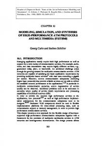
is that, the set of tools available to develop models and simulate them to validate/unravel the actual mechanism of synthesis process require substantial effort. The synthesis of nanoparticles in bulk requires a number of simultaneously occurring steps, shown in Fig. 1.1. In most instances, the material that is to be crystallized into nanocrystals is produced through a reduction reaction. This material in turn nucleates and grows. The most intricate step in the synthesis is often the concurrently occurring processes of nucleation and growth of particles, both of which compete for the same material. Currently homogeneous nucleation based model are in use to describe the burst of nucleation. The applicability of this theory may be limited however, necessitating exploration of other mechanisms to capture nucleation of particles. (One example is provided in Chapter 2.) Once the particles are nucleated, they need to be capped or stabilized, else they undergo simultaneous growth and coagulation processes which invariably produces polydisperse nanoparticles. The amount and composition of stabilizer and capping agents adsorbed on the surface of a particle is an important attribute of a particle along with its volume and composition. A quantitative understanding of the mechanism/processes involved in these systems under well mixed conditions prevailing in batch reactors is possible through Monte Carlo simulations. These are easy to formulate but computationally quite expensive for time varying rates of stochastic processes such as nucleation, growth, and aggregation of particles. (Chapter 3 presents a new approach to carry out Monte Carlo simulations.) Incorporation of quantitative understanding of a synthesis protocols to facilitate development of a engineering scale process for nanoparticle synthesis requires
Chapter 1
7
Metal-1
Nucleation
Growth
PSfrag replacements Reduction Metal-2
Alloy
Stabilization
Coagulation
Coagulated particles
Stable particles
Figure 1.1: Various processes that occur during the synthesis of single component and alloy nanocrystals.
8
Chapter 1
description of the same processes through bivariate, tri-variate, and multi-variate population balance equations so that these can be combined with description of flow field and mixing in reactors to eventually develop optimized processes. Solution of multi-variate population balance equations to obtain spatial evolution of complete particle size distribution in flow reactors and temporal evolution in batch and semi-batch reactors is also computationally extremely demanding. (A new framework to solve multi-variate population balance equations is presented in Chapter 4.) The work presented in this thesis seeks to develop tools and techniques that facilitate quantitative understanding of nanoparticle synthesis. Four contribution made in the thesis are: modeling of widely known protocol of nanoparticle synthesis which required development of new concepts, development of a new approach to carry our Monte-Carlo simulations efficiently using small size systems, development of a new framework to solve multi-dimensional population balances for aggregation, and development of a physical model for digestive ripening which brings together a large body of apparently unrelated experimental findings. The first and last also showcase the complexity associated with the systems one encounters in this field, and some possible ways to address this complexity. The rest of the thesis is organized as follows. Chapter 2 deals with modeling of tannic acid method of synthesis of gold nanoparticles. This protocol is used extensively for synthesis of gold nanoparticles for biomedical applications. We first show that the classical framework provided by the LaMer (LaMer and Dinegar, 1950) type nucleation and growth model based on homogeneous nucleation does not explain the experimental data which has several unusual features. We examined chemistry of tannic acid–tetrachloroauric acid reaction to look for organizer based nucleation mechanism. From among a number of possible pathways that
Chapter 1
9
such an exercise leads to, quite a few were modeled. These failed to quantitatively explain the reported experimental observations. A reaction network of the type used to describe the large number of reactions that occur simultaneously in biological cells was developed. The network served as a guide to isolate reaction pathways which can potentially capture various features present in the experimental data. A minimum network of elementary reactions which captures burst of nucleation, otherwise quite easily captured by the expressions available for homogeneous nucleation (with concentration appearing in an exponential term), was identified. The detailed model developed in the work is the first one for this widely practiced method, and it captures all the reported features. It also makes new predictions and explains why the protocol proposed more than 25 years back has been used without any further modification. Kinetic Monte-Carlo simulations and mean-field population balance models serve as two tools that are used to quantify particulate processes in general. These tools are currently being used to understand synthesis of nanoparticles as well. In kinetic Monte Carlo simulation technique, stochastic events are interspersed with randomly distributed interval of quiescence. Simulations are normally carried out for a large system in which particle population builds to large levels so as to eliminate the effect of statistical fluctuations in small systems. Estimation of interval of quiescence is straightforward for time independent rates of stochastic processes. In nanoparticle synthesis, the concentration of the nucleating species at initial time is zero. As time proceeds, it builds up as governed by the rate of reaction among the precursors. The rate of homogeneous nucleation which is zero at initial time, remains close to zero till the concentration of the nucleating species
10
Chapter 1
far exceeds the saturation concentration. In a narrow range of time, the rate of nucleation increased rapidly and a large number of nuclei are born. The surface area offered by these particles consumes solute for their growth, which rapidly depletes solute concentration and the rate of nucleation again comes to zero. If the birth of nuclei is considered to be a stochastic process, the rate of this process is highly time dependent, with the special difficulty that in the beginning of the process it is zero. If the time dependence of rate processes is not addressed correctly, it leads to (i) situations such as the first interval of quiescence being infinity, and (ii) erroneous simulation results. The problem of formation of first nucleus is resolved in an ad hoc manner in the literature and the time dependence of rate of stochastic processes has been handled through computation intensive algorithms. We propose in Chapter 3 a new approach to carry out MC simulations. It makes use of simulations carried out with systems of extremely small sizes. These simulations yield system size dependent predictions obtained at substantially reduced computational cost. We use a new scaling that we found in this work to construct results for systems of infinite size. An efficient implementation of MC simulation for time dependent rate processes is also developed. In this method. an additional variable is introduced for inter-event evolution. It increases the number of differential equation by one, but dramatically reduces the computational effort required to estimate interval of quiescence for time dependent rate processes. All the above ideas are combined to simulate complete size distribution for simultaneous nucleation and growth of nanoparticles for a system of infinite size from erroneous (system size dependent) simulations carried out with three extremely small size systems. Chapter 4 presents a new framework for solving multidimensional population
Chapter 1
11
balance equations (PBEs) which arise in population balance models that recognize a particle with more than one internal attribute. Solution of one dimensional PBE by discretization, when generalized to n-d PBE, requires discrete elements to be rectangular for 2-d, cuboid for 3-d, and an object with 2n vertices for the solution of n-d PBEs. A new particle born in such a elements is represented though 2n vertices of the element by preserving 2n of its properties. The new framework advances the concept of minimal internal consistency of discretization. It suggests that a n dimensional PBE is a statement of evolution of population of particles while accounting for how n internal attributes of particles change in particulate events. Thus, only a minimum of n+1 attributes of particles need to be preserved perfectly in discrete representation. The discrete elements should therefore be triangles for 2-d, tetrahedrons for 3-d, and an object with n+1 vertices in n-d space for the solution of a n-d PBE. The results obtained show the superiority of this framework over the earlier framework through a comparison of solutions for 2-d and 3-d PBEs. The work also shows that directionality of elements plays a critical role for the solution of multi-dimensional PBEs. A mere change in connectivity of grid points in space which changes their directionality is shown to influence numerical results substantially. This work led to a new discretization of space which has been followed up by others in the group. Chapter 5 deals with digestive ripening of nanoparticles, a technique which has been used extensively in the literature to improve monodispersity of particles produced by techniques which are incapable of producing monodisperse particles themselves. In this technique, particles are boiled under total reflux conditions for a long time to obtain particles of very low values of COV (less than 0.05– 0.10). A critical analysis of the large body of experimental findings reported in the literature is carried out, and a physical model is proposed. It consistently
12
Chapter 1
explains all the reported experimental findings. The overall summary of the work and the scope for future work are presented in Chapter 6.
References Alivisatos, P. (2004) The use of nanocrystals in biological detection. Nature Biotechnology 22, 47–52. Capus, D. J. M. (2003) Nanoparticle markets. Powder Metallurgy 46, 8–8. Eastoe, J., Hollamby, M. J. and Hudson, L. (2006) Recent advances in nanoparticle synthesis with reversed micelles. Advances in Colloid and Interface Science 128–130, 5–15. Gannon, C. J., Patra, C. R., Bhattacharya, R., Mukherjee, P. and Curley, S. A. (2008) Intracellular gold nanoparticles enhance non-invasive radiofrequency thermal destruction of human gastrointestinal cancer cells. Journal of Nanobiotechnology 6, 1–9. Inoue, T., Gunjishima, I. and Okamoto, A. (2007) Synthesis of diametercontrolled carbon nanotubes using centrifugally classified nanoparticle catalysts. Carbon 45, 2164–2170. Jensen, K. F. (2001) Microreaction engineering – is small better? Engineering Science 56, 293–303.
Chemical
Khan, S. A., Gunther, A., Schmidt, M. A. and Jensen, K. F. (2004) Microfluidic synthesis of colloidal silica. Langmuir 20, 8604–8611. Krishnadasan, S., Tovilla, J., Vilar, R., deMello, A. J. and deMello, J. C. (2004) On-line analysis of cdse nanoparticle formation in a continuous flow chip-based microreactor. Journal of Materials Chemistry 14, 2655–2660. Kumar, S., Gandhi, K. S. and Kumar, R. (2006) Modeling of formation of gold nanoparticles by citrate method. Industrial and Engineering Chemistry Research 46, 3128–3136. 13
14
References
LaMer, V. K. and Dinegar, R. H. (1950) Theory, production and mechanism of formation of monodispersed hydrosols. Journal of American Chemical Society 72, 4847–4853. LaVan, D. A., Lynn, D. M. and Langer, R. (2002) Moving smaller in drug discovery and delivery. Nature Reviews 1, 77–84. Law, M., Greene, L. E., Johnson, J. C., Saykally, R. and Yang, P. (2005) Nanowire dye-sensitized solar cells. Nature Materials 4, 455–459. Lewis, N. S. (2007) Toward cost-effective solar energy use. Science 315, 798–801. Lu, W. and Lieber, C. M. (2007) Nanoelectronics from the bottom up. Nature Materials 6, 841–850. Park, J., Joo, J., Kwon, S. G., Jang, Y. and Hyeon, T. (2007) Synthesis of monodisperse spherical nanocrystals. Angewandte Chemie 46, 4630–4660. Qian, X., Peng, X.-H., Ansari, D. O., Yin-Goen, Q., Chen, G. Z., Shin, D. M., Yang, L., Young, A. N., Wang, M. D. and Nie, S. (2008) In vivo tumor targeting and spectroscopic detection with surface-enhanced raman nanoparticle tags. Nature Biotechnology 26, 83–90. Shalom, D., Wootton, R. C. R., Winkle, R. F., Cottam, B. F., Vilar, R., deMello, A. J. and Wilde, C. P. (2007) Synthesis of thiol functionalized gold nanoparticles using a continuous flow microfluidic reactor. Materials Letters 61, 1146– 1150. Stair, P. C. (2008) Advanced synthesis for advancing heterogeneous catalysis. The Journal of Chemical Physics 128, 182507–1–182507–4. Swihart, M. T. (2003) Vapor-phase synthesis of nanoparticles. Current Opinion in Colloid and Interface Science 8, 127–133. Tulloch, G. E. (2004) Light and energy-dye solar cells for the 21st century. Journal of Photochemistry and Photobiology A: Chemistry 164, 209–219. Turkevich, J., Stevenson, P. C. and Hillier, J. (1951) A study of the nucleation and growth processes in the synthesis of colloidal gold. Discussions of Faraday Society 11, 55–75.
References
15
Wagner, V., Dullaart, A., Bock, A.-K. and Zweck, A. (2006) The emerging nanomedicine landscape. Nature Biotechnology 24, 1211–1217.
Chapter 2 Modeling of Citrate-Tannic Acid Method of Synthesis of Gold Nanoparticles 2.1
Introduction
Gold nanoparticles find applications in electronics (Schmid and Chi, 1998; Zhao et al., 1992), catalysis (Haruta, 2004), biomedical (Jahn, 1999; Xu et al., 2006), electrochemical (Guo and Wang, 2007), and a number of other fields. Given the diversity of applications gold nanoparticles facilitate, they have emerged as an important building block for nanotechnology (Brust and Kiely, 2002). For details on synthesis, properties and applications of gold nanoparticles the reader is referred to review article by Masala and Seshadri (2004); Cushing et al. (2004); Daniel and Astruc (2004); Park et al. (2007), and books by Hayat (1989) and Schmid (2004), and a large number of references available therein. A number of protocols are available for the synthesis of gold nanoparticles. The wet synthesis route which involves mixing of liquids containing reactive precursors is among the most energy efficient ones. This route also does not require specialized equipment and can produce spherical nanoparticles of small 17
18
Chapter 2
size with acceptably low polydispersity. Wet synthesis of nanoparticles can be carried out both in organic and aqueous phase, depending on the requirements of the end application. For example, thiol capped gold nanoparticles synthesized in organic phase are used to obtain self-assembled structures (Jiang et al., 2001), whereas gold nanoparticles synthesized in aqueous phase are useful in biomedical applications (Jahn, 1999) such as bio-assay (Schofield et al., 2006), cytochemistry (Slot and Geuze, 1985), tumor detection (Copland et al., 2004), etc. As pointed out in Chapter 1, most of these applications require nearly monodisperse particles of small sizes. A number of synthesis methods are reported in the literature for the aqueous phase synthesis of gold nanoparticles (Masala and Seshadri, 2004). Only a few of these are useful in preparing small monodisperse stable spherical particles reproducibly (Hayat, 1989). Two widely used aqueous phase synthesis methods are: the citrate method of Turkevich et al. (1951) and the citrate-tannic acid method of Muhlpfordt (1982), modified by Slot and Geuze (1985) to its present widely used form. The citrate method uses chloroauric acid and sodium citrate as precursors. The mean diameter of particles synthesized using this method can be controlled by varying the amount of sodium citrate added to the system; a decrease in the amount added over a factor of four increases the particle size from ∼ 15 nm to 170 nm and decreases the number of nuclei generated by more than a thousand times (Frens, 1973; Kumar et al., 2006). The use of tannic acid for the synthesis of gold nanoparticles is an age old process (Weiser, 1933). The use of sodium citrate and tannic acid together to reduce chloroauric acid is a relatively recent development. It was first proposed by Muhlpfordt (1982) as an alternative to the use of white phosphorous (Horisberger and Rosset, 1977) to synthesize gold nanoparticles of relatively small sizes
Chapter 2
19
(∼5 nm). According to the method proposed by Muhlpfordt (1982), a 100 ml solution of chloroauric acid is brought to boil in a 500 ml Duran-glass Erlenmeyer flask in exactly 6.5 minutes. The solution is stirred vigorously throughout. The reducing agent solution (2.45 ml) consisting of sodium citrate and tannic acid at room temperature is added to the flask. Boiling is continued for another 5 minutes after which the solution is cooled under tap water and transferred to polypropylene bottles for storage at 4o C. This process led to the synthesis of stable gold nanoparticles with a mean size of 5.7 nm and a polydispersity (coefficient of variance, COV) of 25%. Various attempts to relax this strict protocol such as the use of glassware of different type and capacity, different volume of reaction mixture, different mode of addition of reducing agent, etc. led to the formation of bigger particles, in size range of 8.4–15.0 nm. This strict protocol, although with poorly understood rationale for many of its steps, marked the shift to the use of less harmful chemicals to synthesize small size nanoparticles.
Slot and Geuze (1985) modified this protocol to produce nearly monodisperse particles of different mean diameters by using a recipe which does not require glassware of specified type and capacity. The mean size of nearly monodisperse nanoparticles can be tuned from 3 to 17 nm merely by changing the amount of tannic acid added to the reaction system. The ease with which good quality particles of different diameters can be produced has made the citrate-tannic acid method as the method of choice for synthesizing aqueous phase monodisperse (COV ≈0.05) gold nanoparticles of small sizes. These particles are especially important for applications like medical imaging and multiple labeling cytochemistry (Slot and Geuze, 1985). It has not been possible to produce water soluble nanoparticles of such small sizes through other simpler methods. The recent efforts (Hussain et al., 2005) suggest that this situation may change in future.
20
Chapter 2 Despite the widespread use of citrate and citrate-tannic acid methods, a quan-
titative understanding of the processes involved in the synthesis of nanoparticles is quite poor. Although the protocol of Slot and Geuze (1985) is more general than that of Muhlpfordt (1982), the large scale synthesis following the former protocol is also undertaken in large size vessels of specified shape and capacity to maintain reproducibility (Slot and Geuze, 1985). Increasing demand for nanoparticles as building blocks requires larger quantities of nanoparticles of controlled size and polydispersity to be produced. These require scale up of batch protocols or continuous mode of operations.
Recent developments like synthesis of gold nanoparticles in microchannel reactors (Shalom et al., 2007) open up the possibility of continuous synthesis of nanoparticles in a scaled down but more controlled manner. Such processes can become superior to the batch mode synthesis provided reproducible mixing and ease of maintaining desirable temperature profile in flow direction can be used advantageously to compensate for poor mixing in microchannel reactors. Effective control of process parameters to produce particles of desired quality is an important issue. Progress on both these fronts requires a quantitative understanding of the synthesis of gold nanoparticles through the well established protocols. Kumar et al. (2006) have recently developed a detailed quantitative model for the synthesis of gold nanoparticles using the citrate method. The model explains the steep increase in particle size with a decrease in the concentration of reducing agent through rapid degradation of dicarboxy acetone, an intermediate that acts as an organizer of gold atoms for nucleation to commence (Turkevich et al., 1951). The model also captures the presence of a minimum in particle size (Chow and Zukoski, 1994) with respect to the concentration of chloroauric acid.
Chapter 2
21
We present in this chapter the first quantitative model for the synthesis of gold nanoparticles using the citrate-tannic acid method of Slot and Geuze (1985). Homogeneous nucleation and particle growth based model (LaMer model) does not explain the experimental findings. The model developed in the present work considers detailed reactions involved in the synthesis process. It assigns two roles to tannic acid: fast reduction of chloroauric acid leading to the formation of dimers of gold atoms, and organization of these dimers to produce nuclei on which adsorption and surface reaction limited growth takes place. The model explains the experimental data of Slot and Geuze (1985) quite well. It also correctly captures the effect of scaling up or down the concentration of all the species involved in synthesis (Kalidas, 2008), and predicts particle growth to be limited by surface reaction at high concentration of tannic acid and rate of adsorption of gold species at low concentrations.
2.2
Salient Features of Tannic Acid Method
The protocol of Slot and Geuze (1985) to synthesize gold nanoparticles is quite easy to follow. Initially, 80 ml of 0.01% chloroauric acid solution and 20 ml of reducing agent mixture containing 4 ml of 1% sodium citrate and 0-5ml of 1% tannic acid are taken. The two aqueous phases are mixed rapidly under vigorous stirring at a constant temperature of 60o C. For higher amounts of tannic acid (2– 5 ml) in the reducing solution, the reaction mixture turns ruby red immediately after the two aqueous phases are added. The time required for the appearance of color increases progressively with a decrease in the amount of tannic acid below 2 ml. In all the cases, the reaction mixture is boiled before it is finally cooled under tap water. The pH and temperature are found to be important parameters for this protocol. When the amount of tannic acid added is large,
22
Chapter 2
25 mM potassium carbonate solution of volume equal to that of tannic acid is added to the reducing mixture to maintain the pH. As mentioned earlier, the diameter of gold nanoparticles can be varied by changing the amount of tannic acid. This variation is presented in Table 2.1. It can be seen from the table that the mean particle diameter is ∼ 3.2 nm when 5 ml of tannic acid is added. With a progressive decrease in the amount of tannic acid added to 0.01 ml, the mean particle diameter increases to 17 nm which is similar to that produced by the citrate method. A five hundred times decrease in the concentration of tannic acid thus produces a five fold increase in average particle diameter. Some of the other variables pertinent to the synthesis procedure, e.g. moles of tannic acid added, moles of nanoparticles formed, and the number of molecules of tannic acid required to produce one particle, defined as ratio R, are also presented in the same table. The table shows that a decrease in concentration of tannic acid over 500 times changes the value of R by a factor of 3.3, from 1200 to 360. Slot and Geuze (1985) explained their observation of substantial increase in particle size with a decrease in the amount of tannic acid added by invoking homogenous nucleation. They proposed that the reduction of chloroauric acid by tannic acid produces supersaturated molecular solution of gold atoms. The concentration of these atoms increases until nucleation occurs. The growth of nuclei into particles occurs by condensation of gold onto the surface of nuclei and growing particles. This picture is translated into a mathematical model, presented in Appendix A. Predictions of this model are obtained for three expressions available in the literature for homogenous nucleation, and surface processes controlled particle growth. The results presented in the appendix show that a homogenous nucleation based model fails to explain the observed variation of particle size
Chapter 2 TA(ml)
23 Dia(nm)
Approx # of
Mole
Mole
Mol TA/
atom/particle
of NP
of TA
Mol NP(R)
5.000
3.2
976
2.51E-08 30.0E-6
1195
2.500
3.5
1278
1.92E-08 15.0E-6
781
1.000
4.6
2900
8.45E-09 6.00E-6
710
0.500
5.8
5665
4.32E-09 3.00E-6
694
0.250
7.5
10665
2.30E-09 1.50E-6
652
0.080
10.0
29800
8.22E-10 0.48E-6
583
0.050
10.5
34497
7.10E-10 0.30E-6
422
0.025
13.0
65470
3.74E-10 0.15E-6
401
0.010
17.0
146330
1.67E-10 0.60E-7
359
Table 2.1: Experimental data of Slot and Geuze (1985) and calculation of the number of tannic acid molecule per gold nanoparticles (R) for different amounts of tannic acid added to the reaction mixture.
with concentration of tannic acid, even when the parameters of the model are varied widely. In view of the above, we examine in the next section various processes involved in the synthesis of gold nanoparticles for the citrate-tannic acid method.
2.3
Model Development
Tannic acid is a well known reducing agent for many metal salts (Haslem, 1996), and is known to reduce chloroauric acid into gold nanoparticles even in the absence of any other reducing or stabilizing agent (Weiser, 1933). Sodium citrate present in the reaction mixture can also reduce chloroauric acid into gold nanoparticles but as the reduction is orders of magnitude slower than that of tannic acid (Turkevich et al., 1951), we shall consider tannic acid to be the principal
24
Chapter 2
reducing agent in the system, as suggested by Slot and Geuze (1985).
2.3.1
Mechanism of Reduction
Tannic acid is an oligomer of gallic acid. Its chemical structure is shown in Fig. 2.1. The ability of tannic acid to act as a reducing agent in a reaction is
Figure 2.1: Chemical structure of tannic acid molecule. Source: http://www. chinaphytochemicals.com
due to the –OH groups of the gallic acid units which are oxidized to C=O to release one proton for every –OH group for reduction to take place. Gallic acid units in tannic acid have a pair of adjacent –OH groups for the interior units and three such groups for the peripheral units. It has been shown recently by Yoosaf et al. (2007) that for reduction to take place, a pair of adjacent –OH group must oxidize together. The non-adjacent pairs of –OH groups or a single –OH group are shown by them to have no reducing power. Hence the third –OH group, if present, for example, for the peripheral gallic acid units, does not take part in the reaction. In the light of the above, we propose the following mechanism for
Chapter 2
25
the reduction of chloroauric acid into elemental gold. Initially, gold is made available in the reaction mixture as a trivalent ion (Au3+ ). The first step for reduction must therefore involve oxidation of a pair of –OH groups to reduce trivalent gold in chloroauric acid to monovalent gold on any one of the gallic acid units. Further reduction of monovalent gold requires two Au+1 units to come together in the vicinity of another pair of unreacted –OH groups in a nearby gallic acid unit. In general, the probability of such event to occur is small in a dilute solution of chloroauric acid and reduction reaction is likely to proceed at a slower rate. Two Au+1 units in proximity of each other, at distances of the order of a few nanometers, however attract each other with an energy of interaction of the same order as that of a hydrogen bond (Mendizabal et al., 2003). This effect is widely known as the “aurophilic effect” (Schmidbaur, 1990). Thus, it appears possible that two Au+1 located on the same tannic acid attract each other and react with a pair of –OH group as a dimer. The special arrangement of the gallic acid units inside a tannic acid molecule, shown in Fig. 2.2, is such that three gallic acid units remain in close proximity of each other in 3D space. We therefore propose that two nearby Au+1 units come together due to the aurophilic effect and react with the third gallic acid unit in their vicinity. These three gallic units act as an independent reaction site. The other such composite units in the same molecule of tannic acid are assumed to act independently of each other. We will call one such composite unit as an ‘unreacted arm’ prior to its participation in reduction reaction. This two step reduction is shown in Fig. 2.3. There are three unreacted arms in a single unreacted tannic acid molecule. The schematic representation of an unreacted tannic acid molecule is shown in the top left side of Fig. 2.4; the unreacted arms are represented by empty circles.
26
Chapter 2
Figure 2.2: Location of three nearest gallic acid units inside a tannic acid molecule which take part in reduction process together. PSfrag replacements Step-1 OH Au+3 Au2
O
Au+1 O
OH
PSfrag replacements Step-2
OH
OH
Step-2 Au
+3
OH Au+1 Au+1 OH
Step-1 OH
O Au2 O OH
Figure 2.3: Reduction of trivalent gold into elemental gold through the two step mechanism.
Chapter 2
27
We quantify the three step reduction process for one unreacted arm, as discussed above, by a single rate which represents the rate of the slowest step in this process. The whole reduction process for one arm produces a pair of completely reduced gold atoms by oxidation of three gallic acid units in it. This process is shown in detail in Fig. 2.3.
2Au+3
2Au+3
PSfrag replacements
2Au+3
Figure 2.4: Representation of the reduction process through a single step loading reaction, and complete loading of a tannic acid molecule through three successive loading reactions.
This reduction mechanism produces three pairs of C=O groups per pair of Au0 formed through reduction. These C=O groups in acetone are known to offer short term stability to the gold nanoparticles (Li et al., 2003). We consider that the gold dimers formed stay close to one of the C=O groups. The reduction process is thus viewed as transformation of an unreacted arm of tannic acid to an arm loaded with a protected dimer of gold atoms. This is shown in Fig. 2.4 through transformation of an empty circle to a filled one.
28
Chapter 2
2.3.2
Mechanism of Nucleation
The gold dimer in a loaded arm is weakly bonded to the oxidized part of the tannic acid molecule. There are two possible ways in which tannic acid as an organizer molecule can facilitate nucleation to occur. When second arm of a tannic acid molecule gets loaded with a dimer of gold atoms, the new tannic acid species has potential to nucleate. If nucleation through this step occurs at a slow rate, it is possible for the third arm of the same tannic acid molecule also to get loaded with a dimer of gold atom which then nucleates. This situation is similar to the formation of nanoparticles in reverse micelles (Singh et al., 2003), where solute molecules offer very high degree of supersaturation inside a tiny solvent pool. The tannic acid molecule thus acts as an organizer for nucleation events to take place. The nucleation mechanism discussed above is presented schematically in Fig. 2.5, and is called organizer mechanism. The other mechanism through which tannic acid molecule can facilitate nucleation to occur is when two molecules of tannic acid, each with at least one arm loaded with a dimer of gold atoms, come in the proximity of each other due to the Brownian motion, and form a nucleus. The rate of this process is governed by the second order collision rate of the loaded tannic acid species. This nucleation mechanisms is presented schematically in Fig. 2.6. The nuclei so formed are in the vicinity of C=O groups and hence assumed to be stable. As the tannic acid molecule has an open structure, the citrate molecules are assumed to freely move in and out and stabilize nuclei by getting adsorbed on it. The growing gold nanoparticle is therefore considered to be stable against coagulation at all times. Since the reduction of chloroauric acid by tannic acid occurs at a much faster rate than that by sodium citrate, the formation of nuclei is solely determined
Chapter 2
29
by the concentration of tannic acid. This is the case even for the lowest concentration of tannic acid used by Slot and Geuze (1985) in their experiments. As speculated by the authors, this is the reason why the particle diameter obtained for the lowest concentration of tannic acid is larger than the diameter obtained when no tannic acid is used. If some nuclei are produced by tannic acid, gold reduced by citrate will deposit on these and will not lead to formation of new nuclei. Nucleation
Nucleation
PSfrag replacements 2Au+3 Figure 2.5: Nucleation of doubly and triply loaded species. A filled circle represents an arm loaded with a dimer of gold atoms.
2.3.3
Mechanism of Growth
Gold is reduced solely by tannic acid if the latter is present in adequate amount. In such a situation, both nucleation and growth of particles are controlled by tannic acid; sodium citrate acts only as a stabilizer and prevents coagulation of particles. Tannic acid mediated growth of particles occurs when tannic acid species loaded with one or more dimers of gold atoms diffuse to the surface
30
Chapter 2
PSfrag replacements 2Au+3 Figure 2.6: Nucleation through collision of loaded tannic acid species: A filled circle represents an arm loaded with a dimer of gold atoms. A half filled circle indicates that the arm could be empty, loaded or unreacted.
Chapter 2
31
of a particle and give away the dimer to the particle, and the unloaded tannic acid diffuses back. Species with any number of loaded arm may participate in the growth process. Once a loaded species comes in contact with the solid surface, it is assumed to lose all the gold it has before leaving the surface. Growth of particles thus occurs through a multiple-step process, shown in Fig. 2.7. We discuss these steps in detail now. Steps 1 and 5 shown in the figure are mass transfer resistances. Steps 2 and 4 represent the process of adsorption of loaded and desorption of unloaded tannic acid molecules. Step 3 is the transfer of gold dimer to the crystal from the loaded tannic acid molecule. This step is the most intricate step in the whole process. Tannic acid is a big and quite open molecule. Inside this large molecule of diameter approximately 3 nm, a relatively small size dimer of gold atoms is held by weak binding forces of C=O groups. Assimilation of this dimer into the metal crystal requires either the dimer to traverse through the tannic acid molecule to the particle surface or reorientation of the loaded tannic acid molecule to a configuration which facilitates release of the dimer to the particle. Such a step is likely to be the rate limiting step. Chan et al. (1976) have studied micellar assisted solubilization of fatty acid and described the process through similar five step mechanisms. They have derived expressions for the overall rate of reaction for different steps being the rate limiting steps. We have derived similar expressions for the present case. These are presented in Tab. 2.2. Given the nature of reactions involved in the present system, as discussed above, and the small size of nanoparticles for which diffusion limited flux is very high (approaches infinity as particle size approaches zero), the particle growth is expected to be controlled by (i) the adsorption of the loaded tannic acid, and (ii) the release of the dimer to the particle surface, either through its movement
32
Chapter 2
Tb PSfrag replacements
Tb
Ti 1
Ts
3
5
Ts
Ti
2 4
Figure 2.7: Growth of a gold nanoparticle through multi-step mechanism: Various steps involved in the growth process are mass transfer (step-1 and step-5), adsorption-desorption (steps-2 and 4) of active tannic acid species on surface and surface integration (step-3).
Rate limiting step
Form of growth rate expression
Adsorption
k g Tb kd + Tb k a Tb
Mass transfer with Sh=2.0
k L Tb
Adsorption and surface reaction
Table 2.2: The form of the growth rate expression obtained by considering different steps shown in Fig. 2.7 to be rate limiting. The quantities ka ,kg ,kd and kL are constants and Tb is the bulk concentration of the loaded tannic acid species.
Chapter 2
33
across the adsorbed molecule of tannic acid or correct orientation of the adsorbed tannic acid molecule on the particle surface. The model however considers all the five steps to ensure that particle growth does not occur at a rate faster than the fastest possible growth permitted by diffusion step.
2.3.4
Role of Sodium Citrate
As discussed before, citrate does not play a role in determining the number of nuclei. The latter is controlled by the reduction of chloroauric acid with tannic acid alone. As tannic acid is a protecting colloid (Weiser, 1933) and citrate has a strong stabilization effect, we consider the particles in the present system to be stable against coagulation at all times. When the concentration of tannic acid used is stoichiometrically less than that required for complete reduction of trivalent gold added initially, the residual gold is reduced by sodium citrate. The citrate induced growth at 600 C is however much slower than the tannic acid induced growth (Slot and Geuze, 1985). Near final size particles are formed almost instantaneously in the reaction mixture to which stoichiometrically required amount of tannic acid is added. A decrease in the amount of tannic acid added below that required stoichiometrically increases the time required for the appearance of surface plasmon resonance (Slot and Geuze, 1985). Although the nuclei are formed immediately after tannic acid is added, their presence does not show up in spectroscopic measurements due to their very small size (Wilcoxon et al., 1993). These nuclei take considerable time to grow to final sizes as the reduction of chloroauric acid with sodium citrate is slow. It is therefore reasonable to consider particle growth in such situations to occur through two growth processes operating at two different time scales. The growth of particles in the concentration regime of stoichiometrically de-
34
Chapter 2
ficient amount of tannic acid is also considered to be controlled by the surface processes, in agreement with the model of Kumar et al. (2006) for the citrate method of synthesis. Due to the low rate of reduction of chloroauric acid with citrate and the presence of nuclei formed through reduction of chloroauric acid with tannic acid on which gold reduced by sodium citrate can deposit, no further nucleation of particles is likely. Thus, at any given point of time in this regime, the number of particles remains constant and the diameter of particles increases at the same linear rate for particles of all sizes. The citrate mediated growth of nanoparticles therefore increases the average size of particles without changing the standard deviation or the breadth of the particle size distribution.
2.4
Model Equations
Mixing of precursors to synthesize nanoparticles introduces two active species into the system: chloroauric acid and unreacted tannic acid (with three unreacted arms). As reaction proceeds, the unreacted arms of the tannic acid react and get loaded with gold. Eventually, the loaded arms give away their gold, either through nucleation or growth, and produce what we term here as empty arms. Such arms have no direct role left for them in the synthesis process. As time proceeds, different species of tannic acid, differing in number of loaded and unreacted arms appear in the reaction mixture. A tannic acid molecule is therefore denoted by Tij where the subscript i represents the number of unreacted arms (i = 0, 1, 2, or 3) and j represents the number of loaded arms (j = 0, 1, 2, or 3). Initially, we have non-zero population of only T30 . All the other forms of tannic acid are produced only after the first reaction proceeds. The particles present in the system are denoted by Pi where i is the number of dimers of gold present in a particle. As a nucleus can be formed both by a single molecule of
Chapter 2
35
tannic acid with two and three arms loaded with dimer of gold atoms, and by the collision of two tannic acid species with at least one arm loaded with dimer of gold atoms in each, they contribute to the Pi , i = 2, 3, . . . , 6 particle classes respectively. A schematic of different species present in the reaction mixture is shown Fig. 2.8.
PSfrag replacements
T30
T20
T21
T11
T12
T03
T00
T10
T01
T02
P2
P3
Pn
Figure 2.8: Various species present in the system during the synthesis of nanoparticles by tannic acid reduction.
Tannic acid can play the role of an organizer in a number of ways to produce nuclei. Following the model of Kumar et al. (2006) for citrate method of synthesis of gold nanoparticles (Turkevich et al., 1951), it was considered that when a molecule of tannic acid already loaded with a dimer of gold atoms further reduces gold ions to form another dimer of gold atoms, all the four atoms
36
Chapter 2
of gold, weakly held by the tannic acid molecule, come together and nucleate. These nuclei grow to bigger sizes by assimilating the gold dimers present in tannic acid molecules. A mathematical model corresponding to this picture, shown schematically in Fig. 2.9 was developed. This model is present in detail in Appendix B. The model predictions show that it failed to even qualitatively capture all the features present in the experimental data—nucleation was predicted to occur all through the synthesis process at low concentrations of tannic acid, leading to unrealistic particle size distributions. In order to a capture a nucleation phase which lasts only for a short while, the second order mechanism of nucleation discussed above was considered (a schematic of the mechanism is shown in Fig. 2.10). An equivalent mathematical model was developed. This model is presented in detail in Appendix C. This model also failed to capture all the features present in the experimental data. It lead to predictions of very low poly-dispersity and required the rate constant for binary collision leading to nucleation to be significantly larger than that permitted by Brownian motion of tannic acid species. A model is expected to capture the following features present in the experimental data quantitatively: variation of average particle size with concentration of tannic acid, mono-modal size distribution, acceptable predictions of coefficient of variance and particle synthesis to be nearly over on time scale of seconds for high concentrations of tannic acid. These predictions should be obtained with permissible values of rate constants. A number of other unsuccessful attempts with single and multi-step mechanisms finally led to the development of the following approach. A reaction network similar to the one used in the literature to describe a large number of reactions that take place in a biological cell was developed. Fig-
Chapter 2
37
Au+3
Au+3
Reduction
Reduction
Instantaneous PSfrag replacements
Nucleation
Growth Figure 2.9: Schematic representation of the synthesis process for instantaneous nucleation of doubly loaded tannic acid species as the only route to the formation of nuclei. The dotted circle represents an unreacted or empty arm while the half filled circle represents an unreacted, loaded or empty arm
38
Chapter 2 Reduction Au+3
Nucleation PSfrag replacements
Growth Figure 2.10: Schematic representation of the synthesis process for collision between loaded tannic acid species being the principal route for nucleation. The dotted circle represents an unreacted or empty arm
ure 2.11 shows this network. It includes all possible pathways which employ tannic acid as an organizer and a reducing agent for nucleation and growth of gold nanoparticles. Solid arrows indicate conversion of one type of species into another through reduction. Solid bifurcated arrows represent nucleation pathways; the number of curved arrows attached shows the number of nucleation mechanism operational. The dashed arrows represent transformation of species as they contribute to growth of particles. All the pathways involving dashed circles represent processes in which two loaded molecules of tannic acid participate. Dashed circles with three arms represent all the species of tannic acid with at least one arm loaded with a dimer of gold. Filled hexagons represent nuclei formed by both the nucleation mechanisms.
Thus, all the arrows except the curved dashed one, represent first order mech-
Chapter 2
39
T30 PSfrag replacements R30
T21
R21
T20
G21
T12 R20 G12
T11
G11 T10
R11 R12 R10
N12
T01
T03
T02 G01
G03
N03
G02
N02 T00
Figure 2.11: The interaction among various tannic acid species represented through a network of reactions (complete network). Solid, dotted and curved arrows represents reduction, growth and nucleation pathway respectively.
40
Chapter 2
anism with respect to the tannic acid species, and curved dashed arrows represent second order reactions with respect to the tannic acid species. The second order reactions among various species of tannic acid were already tried in an earlier model (Appendix C). Since it does not explain the experimental observations, we will not consider second order reactions in the detailed model that follows. A slightly reduced reaction network omitting the second order mechanism is shown in Fig 2.12 A reaction pathway which permits nucleation and growth of particles at single or multiple stages in a multi-step process can potentially mimic burst of nucleation through self-limiting nucleation. In the early stages of synthesis, when particles are yet to be born and the surface area offered by them for growth is not available, such a pathway permits reaction flux to produce only nuclei. Once enough number of nuclei are born, the surface area offered by them results in diversion of reaction flux to growth of particles and as surface area of particles is increased, diversion of reaction is complete and nucleation comes to a near halt. The left limb of the reaction network shown in Fig. 2.12 offers one such pathway. In the following, a general mathematical model based on the complete reaction network shown in Fig. 2.12 is developed. The general model, guided by the network shown in the figure for desired flow of gold atoms through tannic acid species is developed to obtain model predictions. The notation used to represent various species involved in reactions is shown in Fig. 2.8. With the help of this notation, the reduction of trivalent gold to elemental gold can be written as: k
Tij + 2Au+3 →r Ti−1,j+1
i≥1
(2.1)
The rate of this reaction is assumed to be first order with respect to Tij and second order with respect to the Au+3 . Hence, the rate of the reaction, Rij is
Chapter 2
41
T30 PSfrag replacements R30
T21
R21
T20
G21
T12 R20 G12
G11
T11
T10 R11 R12
N12
R10
T01
T03
T02 G01
G03
N03
G02
N02 T00
Figure 2.12: The interaction among various tannic acid species represented through a network of reactions (reduced network). Solid, dotted and curved arrows represents reduction, growth and nucleation pathway respectively.
42
Chapter 2
given by: Rij = kr [Au+3 ]2 Tij
i≥1
(2.2)
As mentioned earlier, nucleation is a rate process and occurs through reaction knj
Tij −→ Pj + Ti0
j = 2, 3
(2.3)
This process has been assumed to be first order with a rate constant knj . The rate of nucleation can be written as: Nij = knj Tij
j = 2, 3
(2.4)
Similarly, the growth rate per unit area due to the species Tij can be written as: Gij =
kg Tij∗ kd + Tij∗
j≥1
(2.5)
where unknown Tij∗ is estimated by equating diffusive flux with the rate of growth. kL (Tij − Tij∗ ) = Gij
kg Tij∗ kd + Tij∗
(2.6)
The rate of appearance and disappearance of various species can be written as: T˙00 = N03 + N02 + G0 A
(2.7a)
T˙01 = R10 − G01 A
(2.7b)
T˙02 = R11 − N02 − G02 A
(2.7c)
T˙03 = R12 − N03 − G03 A
(2.7d)
T˙10 = −R10 + N12 + G1 A
(2.7e)
T˙20 = −R20 + G21 A
(2.7f)
T˙30 = −R30
(2.7g)
Chapter 2
43 T˙11 = R20 − R11 − G11 A
(2.7h)
T˙12 = R21 − R12 − N12 − G12 A
(2.7i)
T˙21 = R30 − R21 − G21 A
(2.7j)
M˙ 3 = −2R
(2.7k)
P˙2 = N02 + N12 − GA2 P2
(2.7l)
P˙3 = N03 − GA3 P3 + G1 A2 P2
(2.7m)
P˙4 = −GA4 P4 + G1 A3 P3 + G2 A2 P2
(2.7n)
P˙ i = −GAi Pi + G1 Ai−1 Pi−1 + G2 Ai−2 Pi−2 + G3 Ai−3 Pi−3
i = 5, · · · imax (2.7o)
where R=
3 X 2 X
Ri,j
(2.8)
j = 1, 2, 3
(2.9)
i=1 j=0
Gj =
2 X
Gi,j
i=0
and
G=
3 X
Gi
(2.10)
j=1
Ai is the area corresponding to a mole of particle having i dimer units. The total surface area per unit volume of reaction mixture, A, is therefore given by: A=
iX max
A i Pi
(2.11)
i=2
Equation 2.7o is a population balance equation (PBE) for pure growth process in discrete domain. The number of discrete PBEs required to be solved depends on the number of gold atoms in the largest size particle formed. While this number is reasonably small for small size particles (∼3 nm), it can be unmanageably large for large size particles. Simulation of synthesis of large particles till its full grown state through discrete description is impractical, and continuous
44
Chapter 2
description is needed. The latter however requires discretization of the continuous PBE consisting of convective terms corresponding to particle growth (Kumar and Ramkrishna, 1997) to solve it. This technique is numerically somewhat involved. Instead, an alternative and computationally quite efficient technique is used here. We shall discuss this next. The number of particles formed is determined by the self-limiting nucleation which occurs early in the synthesis process. The free gold formed at later times through the reduction by either tannic acid or sodium citrate continues to deposit on the existing particles. No new particles are born. Thus, if at the end of the nucleation phase at time t, the amount of gold converted to particles is Mt , then X i
πd3i Pi (t) ρm = M t 6
(2.12)
where Pi (t) is the number of particles with i units of gold dimers in them and di is their diameter at time t. For surface process controlled growth of particles, d (πd3i /6) = d2i f (t) dt
(2.13)
Function f (t) includes time dependent driving force and other constants which are the same for particles of all sizes. Equation 2.13 can be integrated to obtain particle size at final time after all the gold is exhausted as (di )f = di + δ
(2.14)
The unknown δ is the same for particles of all size present at time t. If the total amount of gold deposited on particles after the completion of the growth process is Mf , then
X i
Pi (t)
π(di + δ)3 ρm = M f 6
(2.15)
Subtracting eq. 2.12 from eq. 2.15 we obtain: δ3
X i
Pi + 3δ 2
X i
Pi di + 3δ
X i
Pi d2i + (Mt − Mf )
6 =0 πρm
(2.16)
Chapter 2
45
which can be solved to obtain δ. The estimated value of δ can be used to construct the final particle size distribution. In the present case, with surface process controlled growth of particles, it only involves shifting of the entire size distribution along the particle diameter axis by amount δ. The final mean diameter is thus simply given by d¯f = d¯t + δ
(2.17)
Since all the particle diameters, including the mean diameter, increase by the same amount, the standard deviation of the size distribution does not changes during the course of growth. The present work uses the above approach to predict the final mean particle size and the coefficient of variance, which are compared with the experimental data reported in the literature. Although not discussed here, the above approach of obtaining particle size distribution after nucleation comes to halt is also extendable to any other growth law.
2.5
Results and Discussion
The model equations (eqs 2.7a–2.7o) need to be solved simultaneously to obtain model predictions. Equation 2.7o for particle growth needs to be solved for large enough size of particles to ensure that the largest particle size chosen encompasses the size of the largest particle produced during simulations. As discussed earlier, the size distribution obtained at the end of the nucleation phase is translated along particle diameter axis to simulate deposition of gold on these particles. The additional gold is deposited in proportion to the surface area offered by them. A number of such simulations were carried out for different initial concentrations of tannic acid. For the set of parameter values presented in Table 2.3, the variation of final mean particle diameter with the concentration of tannic acid is shown in
46
Chapter 2 Parameter
Value
Unit
kr
0.2×10³
(mol/m3 )−2 s−1
kg
0.5×10⁻³
(mol/m3 )m−2 s−1
kd
0.2×10⁻⁴
(mol/m3 )
kn2
2.0
s−1
kn3
3.0
s−1
Table 2.3: The best fit values of the parameters used in the simulation to obtain the model predictions shown in Fig. 2.13
Fig. 2.13. The experimental data of Slot and Geuze (1985) are shown by points and the model predictions are shown by the dashes line. The predictions of the model are in quite good agreement over the entire range of concentration of tannic acid reported by Slot and Geuze (1985). More importantly, the model predictions capture various features of the experimental data. First of all, the model predictions follow a near constant slope (power law behavior) on a plot of average particle diameter vs. amount of tannic acid (ml of 1% tannic acid solution added) on log scale in the most of the concentration range of tannic acid, as shown by the experimental data. This feature has not been predicted by other models; all the homogenous nucleation based models predict a faster and non-power law type increase in particle size with a decrease in concentration of tannic acid on same type of plots (please refer to Appendix A). Another feature shown by the experimental data is a decrease in slope for the last few data points in the range of high concentration of tannic acid. This feature has also been captured correctly in the present model. As population balance equation is embedded in the model, this model gives precise information about the particle size distribution. Figure 2.14 shows such
Chapter 2
47
Expt
16
Model
Dia(nm)
8
4 PSfrag replacements
2
0.01
0.1 1 Amount of tannic acid
10
Figure 2.13: Experimental data versus model prediction for the entire range of tannic acid concentration. The amount of tannic acid is in terms of ml of 1% tannic acid solution. The corresponding values of various parameters are shown in table. 2.3.
ag replacements
48
Chapter 2
4e-07 3.5e-07
Frequency(mol/m3 )
3e-07 2.5e-07 2e-07 1.5e-07 1e-07 5e-08 0
1
2
3
4 Dia(nm)
5
6
7
Figure 2.14: Final particle size distribution for the case of addition of 5 ml of tannic acid solution.
Chapter 2
49
a distribution when highest amount of tannic acid (5 ml) has been used. Similar distribution for the lower amount of tannic acid (0.025 ml) has been shown in Fig. 2.15. We observe that the shape of the two distribution is slightly different. The particle size distribution for larger particle shows a longer tail towards the lower size end. This feature results from relatively prolonged nucleation phase during falling rate of nucleation. Unfortunately, the data for particle size distribution is not available from experiments and this feature could not be verified with experimental data. 1.4e-08
Frequency(mol/m3 )
1.2e-08 1e-08 8e-09 6e-09 4e-09 2e-09
PSfrag replacements
0
7
8
9
10 Dia(nm)
11
12
13
Figure 2.15: Final particle size distribution for the case of addition of 0.05 ml of tannic acid solution.
Table 2.4 shows model predicted values of coefficient of variance (COV) along with the experimental data. The model is able to capture the variation in polydispersity with the amount of tannic acid added. The prediction of COV for
50
Chapter 2 Ml of TA
Experimental
Model
2.00
11.7
20
0.50
7.3
16
0.125
6.9
10
0.03
6.3
7
Table 2.4: Comparison of the COV obtained with the detailed network model with the experimentally obtained values. The corresponding prediction for diameters are shown in Fig. 2.13
size distributions with smaller value of mean particle size is somewhat higher, but the corresponding difference in the value of standard deviation is small. For example, COV can vary from 15% to 20% if the standard deviation changes merely by 0.15 nm for particles with a mean size of 3 nm. It is desirable to account for the uncertainty (confidence interval) involved in the measurement of standard deviation, while comparing the quality of model prediction especially for particles of small mean sizes. Nonetheless, the variation in polydispersity as represented by the measured COV is captured well by the model.
2.5.1
Mechanism of Particle Formation
As discussed in section 2.4, inter-conversion of one form of tannic acid to several of the choices available to it through further reaction, nucleation, and particle growth is responsible for the final outcome of the synthesis process. The relative magnitude of nucleation and growth plays the most important role in determining the particle size and size distribution. In this section, we discuss how the complex interactions among various species determine the process of particle synthesis by considering specific examples. In the protocol of Slot and Geuze
Chapter 2
51
(1985), concentration of tannic acid is varied over two orders of magnitude. In order to understand the entire spectrum of interactions that is possible, we shall take two representative cases, one corresponding to the highest amount of tannic acid, and the other corresponding to the lowest one. We shall discuss these cases in turn. The concentration profiles for various species present in the system for the case of highest concentration of tannic acid (5 ml of 1% solution added to the mixture) are shown in Fig. 2.16. The figure shows that starting with species T30 , unreacted tannic acid with three active arms and no loaded arm, initially only three species are produced in the system, T21 , T12 and T03 . These species result from the series reaction route (R30 − R21 − R12 ) shown in Fig. 2.12. Figure 2.16 shows that as time progresses, the concentrations of T12 and T03 build up and nucleation occurs through pathways N12 and N03 . Since the concentration of T12 is much larger than that of T03 , the former plays a dominant role in the formation of nuclei. The nuclei born offer surface area for particle growth to also proceed simultaneously. At this stage in particle synthesis, every pathway in the reaction network comes alive. Nucleation by itself does not deplete the concentration of species T12 substantially. The concentration of species T12 therefore continues to increase steadily in the early stage of nucleation. During this time, the existing nuclei grow at the expense of T21 , T12 and T03 and fresh nuclei are born simultaneously. The growth process observed in such systems resembles autocatalytic reaction. More and more surface is created due to growth (∝ v 2/3 ) and as more surface area becomes available, more material is consumed in growth process. As a result, intermediate species T21 , T12 , and T03 are consumed rapidly through growth process. Concentrations of species T12 , and T03 fall precipitously and this nearly
52
Chapter 2
shuts off the other pathways leading to nucleation. New species T10 and T20 are formed which after further oxidation, lead to formation of T01 and T11 . As species T21 is present at a much higher concentration because it is formed from the large pool of T30 present initially, the relative contribution of species T01 and T11 to particle growth is not significant. The concentration of another species that can potentially lead to formation of nuclei (T02 on the right side of the network) does not build to large enough levels to result in secondary nucleation. This is because the number of intermediates required to form species T02 have other pathways available to them. Once, sufficiently large surface area becomes available in the system, these pathways are preferred over other pathways. The forgoing discussion suggests that species T12 acts in a similar way as the super-saturating species in homogenous nucleation. Until particles are born, the concentration of T12 increases and nuclei are produced. Its consumption through growth process is responsible for the precipitous drop in concentration. One essential difference between the present mechanism and a single step reaction leading to nucleation is that although a significant amount of T12 is consumed by the growth process, the actual growth of particles is mainly governed by another species T21 , not T12 . It can be noted that the nucleation and growth of particles facilitated by T12 have similar dependence on the concentration on T12 . It is the autocatalytic nature of growth of particles which is responsible for the concentration of T12 to drop by two orders of magnitude in a short period of time. The self-limiting nucleation obtained with a series of elementary reactions and autocatalytic growth processes thus captures a burst of nucleation quite well. The same is captured by the classical homogenous nucleation theory by exponential dependence of rate of nucleation on super-saturation. The time evolution of concentration of trivalent gold and particles for the high
Chapter 2
53
0.1
PSfrag replacements
Conc.(mol/m3 )
T01 0.01
T02
0.001
T03 T11
1e-04
T12 T21
1e-05 1e-06 1e-07 1e-08 0.001
0.01
0.1
1
Time(sec) Figure 2.16: Time evolution of concentration of various species of tannic acid for the case of addition of 5 ml of tannic acid solution.
54
Chapter 2 1
1.0e-03 1.0e-04
1.0e-06 1.0e-07
ag replacements
Conc. of particle
Conc. of Au+3
1.0e-05
1.0e-08
Au
+3
0.001
0.01
0.1
1
1.0e-09
Time(sec)
Particle
Figure 2.17: Time evolution of concentration of trivalent gold and particles for the case of addition of 5 ml of tannic acid. All concentrations are in mol/m3
tannic acid concentration case is shown in Fig. 2.17. The nucleation process for this system comes to a halt within a time period of 0.04 second and 70% of gold gets reduced within 0.1 sec. The mean diameter of the particle formed at this time is 2 nm which is capable of producing surface plasmon resonance. These predictions suggest that at high concentration of tannic acid, the nucleation phase is complete even before the particles can be detected using spectroscopic technique. .
The situation is different when concentration of tannic acid is low. This is shown in Fig. 2.18. As the amount of tannic acid is smaller by more than
Chapter 2
55
two orders of magnitude, the concentration of chloroauric acid remains nearly unchanged (shown in Fig. 2.19) during the time it takes to exhaust the reducing capacity of tannic acid. A decrease in concentration of tannic acid by 500 fold decreases the concentration of species T21 species also by the same factor. The concentration of nucleating species T12 also drops by the same factor. Since the concentration of T21 is at a much reduced level than in the previous case, the nuclei born through route N12 do not offer large enough surface area for concentration of T12 to fall precipitously to very low levels. This is also evidenced by the much larger value of the maximum ratio of concentration of species T12 and T21 for this case. As a result of the slow decrease in the rate of nucleation with time, new nuclei with relatively significant population continue to be form in the present case. This explains the higher standard deviation predicted for low concentrations of tannic acid. The continued availability of chloroauric acid allows species T11 and T01 to be formed through the route (T12 → T10 → T01 ) and (T21 → T20 → T11 ) respectively. These species play a dominant role in shaping the size distribution to a bell shaped curve. The conversion of T11 to T02 can potentially provide secondary nucleation through pathway N02 . The presence of large particle surface area activates pathways G11 and G02 to such an extent that pathway N02 suppressed completely.
2.5.2
Effect of Concentration of Reactants
We have already studied the effect of the concentration of tannic acid over the entire range covered in the experiments reported in the literature. We note that the mean particle diameter vs. concentration of tannic acid (Fig. 2.13) shows a single slope in the most of the concentration range studied experimentally. In the range of high concentration of tannic acid (corresponding to addition of more
Chapter 2
0.1
T01
Conc.(mol/m3 )
ag replacements
56
0.01
T02
0.001
T03 T11
1e-04 1e-05
T12 T21
1e-06 1e-07 1e-08 0.001
0.01
0.1
1
Time(sec) Figure 2.18: Time evolution of concentration of various species of tannic acid for the case of addition of 0.01 ml of tannic acid solution.
Chapter 2
57
1
1.0e-05 1.0e-06
1.0e-08 1.0e-09 1.0e-10
PSfrag replacements
Conc. of particle
Conc. of Au+3
1.0e-07
1.0e-11
Au
+3
Particle
0.001
0.01
0.1
1
1.0e-12
Time(sec) Figure 2.19: Time evolution of concentration of trivalent gold and particles for the case of addition of 0.01 ml of tannic acid. All concentrations are in mol/m3
58
Chapter 2
than 1 ml of tannic acid to the reaction mixture), both the experimental data and the model predictions show the decreased dependence of mean particle size on the concentration of tannic acid. It appears from the plot that an increase in the amount of tannic acid added to the reaction mixture beyond 5 ml may lead to a further decrease in mean particle diameter. Slot and Geuze (1985) have not made any statement in this regard, however. We have used the model developed here to simulate the addition of higher amount of tannic acid. The simulation results are presented in Fig. 2.20. The figure shows that the mean particle diameter, instead of approaching an asymptotic value at high concentration of tannic acid, increases with an increase in tannic acid concentration beyond that corresponding to the addition of 5 ml tannic acid to the reaction mixture. The reason for this predicted behavior is as follows. An increase in concentration of tannic acid increases the amount of both T21 , the species responsible for growth of particles in this range of concentration of tannic acid and the nucleating species T12 . An increase in the concentration of tannic acid increases the concentration of T21 which in turn accelerates the particle growth to such an extent that the large surface made available by this process in a short time consumes species T12 also for particle growth (step G12 ), thereby suppressing the parallel nucleation step N12 . The intricate balance between the two processes gives rise to a minimum in particle size. If the increase in concentrations of T21 and T12 with an increase in concentration of tannic acid is such that the increase of concentration of T21 does not rapidly produce very large surface area, the increased concentration of T12 produces larger number of nuclei and the mean particle size decreases. This is what happens as the amount of tannic acid added is increased to 5 ml. A comparison of concentration profile of various species for
Chapter 2
59
Dia(nm)
16
8
4
PSfrag replacements
5 ml of 1% TA solution 2 1e-04
0.001
0.01 0.1 Conc.(mol/m3 )
1
10
100
Figure 2.20: Effect of concentration of tannic acid on the final diameter of the particle over a wide range of concentration of tannic acid.
Chapter 2 1
Tx03
0.1
Tx12
0.01
Conc.(mol/m3 )
ag replacements
60
Tx21
0.001
T503
1e-04
T512
1e-05
T521
1e-06 1e-07 1e-08 0.001
0.01 Time(sec)
0.1
Figure 2.21: Time evolution of concentration of various species of tannic acid for addition of excess tannic acid (indicated by the superscript x) and that for the highest concentration (5 ml of 1% TA) used by Slot and Geuze (1985).
the addition of 5 ml and larger amount of tannic acid is provided in Fig. 2.21. The model predicts that mean particle sizes larger than the minimum possible can be obtained at two concentrations of tannic acid, one smaller and the other larger than the concentration at which optimum occurs. The model also predicts that of the two concentrations, the higher concentration of tannic acid yields particles with somewhat reduced COV than those obtained with lower concentration of tannic acid, as shown in Table 2.5. This is because at higher concentration of tannic acid, the reduced availability of gold at later stages of reduction confines nucleation to a rather small window of time.
Chapter 2
61 Dia(nm) COV(Below 5 ml)
COV(Above 5 ml)
3.5
21
19
4.0
19
13
10.0
8
5
Table 2.5: Model prediction of COV for the same diameter obtained in different concentration regime when the detailed network model is applied over extended range of concentration
It is possible that the use of tannic acid at concentrations larger than the maximum employed by Slot and Geuze (1985), which can yield particles with smaller polydispersity, hinders the binding of protein to gold nanoparticles. We are however unsure about it. An increase in concentration of tannic acid in a different protocol investigated in our group (Kalidas, 2008) produces a minimum in particle size in the same range of concentration of tannic acid as predicted by the present model. Figure 2.36 in Appendix C compares predictions of the two preliminary models presented briefly earlier and discussed in detail in Appendices B and C and the present model for the variation of mean particle with concentration of tannic acid. Figure 2.36 shows that the predictions of the other models in the high concentration range of tannic acid are quite different from each other. We also examine the effect of increasing the concentration of gold, while keeping the concentration of tannic acid constant in the present model. The model predicts the formation of particles of even smaller mean size, but with considerably high polydispersity. For example, addition of 5 ml of tannic acid in standard protocol produces a diameter of 3 nm. A doubling of the concentration of gold produces a particle of diameter 2.6 nm but with a COV of 0.30; the COV
62
Chapter 2
predicted for the standard protocol is 0.21. It is also possible to increase concentrations of both tannic acid and gold while keeping their ratio at the same value as in the standard protocol. Kalidas (2008) have studied this effect and found that an increases in concentration of all the species by a factor of two over the concentrations used in the standard protocol decreases the mean particle diameter. Similarly, when concentrations of all the precursors are halved, a larger value of mean particle diameter is obtained. Figure 2.22 shows the model prediction for the standard protocol and the two variations discussed above. It is clear from the figure that the model successfully captures this feature.
100
Standard Double
Dia(nm)
Half
10
ag replacements
Expt 1 0.001
0.01
0.1 [TA]/[Au]
1
10
Figure 2.22: Effect of scaled up (twice) and scaled down (half) concentrations of all the precursors on average diameter of gold particles for the protocol of Slot and Geuze (1985)
Chapter 2
63 s.f.=0.5
s.f.=1.0
s.f.=2.0
Dia
COV(%)
Dia
COV(%)
Dia
COV(%)
5.44
14
3.44
21
2.64
27
6.11
13
3.62
21
2.60
30
7.5
12
4.27
19
2.9
28
10.4
10
6.17
13
4.2
19
14.3
8.4
10.1
8
7.1
11
18.2
6
15.8
6
12.4
6
Table 2.6: Comparison of the diameter and COV obtained with various scale factors (s.f.). The results presented in a given row corresponds to a fixed ratio of concentrations of two precursors.
The predictions shown in Fig. 2.22 for mean particle size for three values of scale factor (s.f.) are also presented in Table 2.6 along with the predicted values of COV. The table shows an interesting feature. The particles of the same mean size when produced by using higher concentrations (s.f.= 2.0) are more polydisperse. The less concentration of all the species (s.f.= 0.5) results in formation of particles with somewhat lower polydispersity but the smallest mean particle size produced for this scale factor is larger than that obtained for the standard protocol (s.f.= 1.0). The model predictions suggest that there is scope for decreasing the polydispersity of particles with higher mean particle diameter. The synthesis of particles with smaller mean diameter and lower polydispersity than those obtained through the standard protocol appears difficult for this synthesis method.
64
Chapter 2
2.6
Minimal Organizer for Self-limiting Nucleation
In this section, we propose a minimal organizer based reaction network which can capture self-limiting nucleation and other features discussed earlier. The motivation for developing the minimal network is that it can serve as a guide in exploring chemistry/mechanism required to explain the experimental observations when homogeneous nucleation based mechanism does not operate in the system. The detailed discussion presented in the previous section suggests that key to successful prediction of various features of experimental data, particularly self-limiting nucleation, is the multi-step hierarchical mechanism of particle synthesis, supported by the formation of a number of intermediate species. The reaction network presented in Fig. 2.12, derived from detailed consideration of the chemistry of the reaction, has three levels of hierarchy– the three arms of tannic acid species get successively loaded with gold atoms. The lowest level species T30 feeds to the next level species T21 , and so on. A molecule with a minimum of two arms can organize solute atoms on it for nucleation to occur. Until particles are born and sufficient surface area builds up in the system, organizer leads to nucleation through three rate processes: loading of first arm followed by the loading of the second arm, and finally nucleation at a finite rate. Once sufficient surface area builds up in the system, the same species which at initial time led to nucleation begins to participate in growth of the existing particles. As the surface area in the system increases further, the pathways leading to particle growth behave like autocatalytic ones and nucleation gets self-limited (suppressed). Figure 2.23 shows the minimal network discussed in the previous paragraph, with organizer consisting of only two arms. The chemistry dictates that six atoms
T03
T30
Chapter 2
65
T12
T20
T21 R30 R20
R21 R12
T11 R11
G21 G12
T10
G11
T02 R10
T01
G02 G03
T00
N12 N03
G01 N02
Figure 2.23: The reaction network corresponding to the minimal organizer (see text for details)
of gold must be reduced by every molecule of tannic acid. In order to represent the overall stoichiometry correctly for the present case, we consider each of the two arms in this representation to reduce a trimer of gold atoms (which is not in agreement with the detailed chemistry considered, however). The model equations corresponding to the above network are presented below (eq. 2.18a– 2.18i). The expressions for Rij , Nij and Gij are identical to those given earlier through eqs 2.2, 2.4 and 2.5 respectively, the only difference being that each arms gets loaded with three gold atoms instead of two.
66
Chapter 2
T˙00 = N02 + G01 A + G02 A
(2.18a)
T˙01 = R10 − G01 A
(2.18b)
T˙02 = R11 − N02 − G02 A
(2.18c)
T˙10 = −R10 + G11 A
(2.18d)
T˙20 = −R20
(2.18e)
T˙11 = R20 − R11 − G11 A
(2.18f)
M˙ 3 = −3R
(2.18g)
P˙2 = N02 − GA2 P2
(2.18h)
P˙ i = −GAi Pi + GAi−1 Pi−1
(2.18i)
Figure 2.24 shows a comparison of the prediction of the minimal organizer model with the experimental data. The values of all the parameters used to obtain model predictions are the same as those presented in Table 2.3, except for the value of kn2 which is increased to 5.0 s−1 , equal to the sum of two rate constants for two nucleation steps considered in the complete model. It is clear from the figure that the minimal organizer model for self-limiting nucleation predicts experimental data quite well. Although not shown here, it captures all the other features predicted by the detailed model as well. It is important to understand the chemistry of the process. Once the chemistry is understood, it can be represented in more than one way to reach the goals of the modeling activity. If intermediate species can be identified and their concentrations can be measured, some of the rate constants can then be obtained from transient concentration profiles. Simplified representation of a detailed mechanism is useful in such a situation as well. The simplification needs to
Chapter 2
67
Expt
16
Model
Dia(nm)
8
4
PSfrag replacements
2
0.01
0.1 1 Amount of tannic acid
10
Figure 2.24: The experimental data versus model prediction for minimal organizer model. The corresponding reaction network is presented in Fig. 2.23. The amount of tannic acid added is in terms of ml of 1% solution
be developed with care to ensure that the apparent rate constants can be related to the experimentally measured ones. It is also possible to determine apparent rate constants directly from independent experiments.
2.7
Conclusions
Although a number of protocols are available for synthesis of gold nanoparticles, only a few of these can be used for their controlled and reproducible synthesis. One such protocol uses tannic acid as a reducing agent and chloroauric acid
68
Chapter 2
as gold precursor, and sodium citrate as stabilizer. This protocol, already in extensive use to synthesize nanoparticles for medical diagnostics purposes, could also be used for engineering scale synthesis of gold nanoparticles in continuous reactors. A quantitative understanding of this protocol is required before it can be combined with the description of transport processes in a continuous flow reactor to develop an optimum process. Efficient simulation tools are also required to accelerate development towards this goal.
The classical homogeneous nucleation based models tested in this work failed to explain the experimental data available in the literature for this protocol. A detailed investigation of the chemistry of the process reveals that tannic acid acts both as a reducing agent and an organizer (which brings together atoms to facilitate formation of nuclei) for nucleation process. Based on the structure of tannic acid and the reactions it can participate in, it is visualized as consisting of three reduction sites. Each of these sites, called an arm, can be in one of the three states: unreacted, reacted and loaded with a dimer of gold atoms, and reacted and unloaded (empty). A detailed reaction network involving various species of tannic acid is proposed. The tannic acid species with two and three loaded arms are permitted to form nuclei at finite rates. The tannic acid species with one or more loaded arms contribute to growth of particles. The model successfully captures (i) a burst of nucleation over a small time window through self-limiting nucleation mechanism introduced in this work, (ii) bell shaped particle size distribution, (iii) completion of synthesis in about a second at high concentration of tannic acid, and (iv) the variation of mean particle size and breadth of size distribution with changes in concentration of tannic acid. The model predicts a minimum in mean particle size with an increase in concentration of tannic acid, which possibly explains why the original protocol developed more than twenty
Chapter 2
69
five years ago could not be improved upon by others to produce gold nanoparticles of sizes smaller than the smallest size reported originally. The present work also brings out the minimal hierarchical network required for self-limiting nucleation mechanism to become operative. An organizer-cumreducing agent is required to contain a minimum of two arms, which can be in loaded, unloaded, and empty state. Although such a description violates the detailed chemistry of tannic acid synthesis brought out in this work, its predictions for this protocol are nearly the same as those of the the detailed model based on the chemistry of reactions. The minimal model for self-limiting nucleation thus offers itself as an alternative to homogeneous nucleation mechanism, which can possibly be used as a tool to develop model based understanding of synthesis of other types of nanoparticles as well.
2.A 2.A.1
A Homogeneous Nucleation Based Model Introduction
Homogeneous nucleation theory, also known as Classical Nucleation Theory (CNT) is used widely to predict rate of nucleation. Its successful application to explain particle formation in a large variety of systems including nanoparticle synthesis (Teychen and Biscans, 2008; Mirable and Katz, 1977; Singh et al., 2003) has led to appearance of this theory in almost every book available on colloidal chemistry. Although the applicability of this theory as a quantitative one has been questioned by a few (Strey et al., 1986; Liu, 2000), its ability to very easily emulate burst of nucleation, which leads to formation of reasonably monodisperse particles in a number of situations is one of its most important attributes. Several efforts have been made in the recent past to model synthesis of gold
70
Chapter 2
nanoparticles for various protocols using homogeneous nucleation based models (Privman et al., 1999; Robb and Privman, 2008; Park et al., 2001). Goia and Matijevic (1999) prepared concentrated gold colloid of micron size by coagulating nanometer sized primary particles which were produced in-situ by reducing tetrachloroaurate by ascorbic acid.
Privman et al. (1999) modeled this system by
considering homogeneous nucleation of elemental gold to produce primary particles, which in turn get coagulated and sintered to produce bigger secondary particles. Particle growth by deposition of gold atoms has not been considered in this model. The model could predicted the experimental data semi-quantitatively. In the light of the above discussion, it appears possible that the protocol of Slot and Geuze (1985) for synthesis of gold nanoparticles using tannic acid as reducing agent could also be modeled through homogeneous nucleation mechanism. The test of the such a model will be its ability to explain the experimental data on variation of mean particles size with concentration of tannic acid used. The details of the synthesis protocol, as discussed by Slot and Geuze (1985), and its salient features are reviewed in the main chapter.
2.A.2
Development of the Model
Primarily three processes are involved in the synthesis process, reaction, nucleation and growth. The reaction step involves the reductive formation of elemental gold (solute) by chemical reaction between chloroauric acid and tannic acid. As the concentration of solute increases in the system, it exceeds its solubility (Cs ) at one stage. At concentrations just above Cs , the rate of nucleation is practically zero and concentration increases steadily. At a somewhat higher value of concentration (Cs∗ ), the rate of nucleation increases rapidly and in a short span of time, a large number of nuclei are born. These particles start to
Chapter 2
71
grow simultaneously. When the surface area grows to a sufficiently large value, the rate of production of solute fails to keep pace with its consumption through growth process. This brings the supersaturation down and nucleation comes to a halt. The particle growth however continues for a longer period, as long as the solute concentration is maintained above its solubility. These processes are captured schematically in Fig. 2.25. As nucleation occurs only over a quite short window of time, a burst of nucleation is realized with this model. The above mechanistic model is also known as LaMer’s classical model of nucleation and growth (LaMer and Dinegar, 1950). The mechanism of growth of nanocrystal is not understood clearly. The growth of bigger particles (few micron and above) is primarily controlled by mass transfer processes. The growth of smaller particles in comparison is controlled by surface processes—adsorption or assimilation of solute on the surface of a growing crystal (Nielsen, 1964). In the present model, we consider growth to be controlled by adsorption process. The key quantity of interest is the average particle diameter obtained at the end of the synthesis process. As nucleation occurs only over a short interval of time, the average particle diameter is obtainable as soon as nucleation phase is over. The present model is thus simulated only to determine the total number of nuclei formed. The average particle is determined by dividing the total amount of gold reduced at the end of the process by the total number of nuclei formed. The processes discussed above can be represented by the following simple reactions: k
T + G →r A N˙
A→P kg
P +A→M
(2.19) (2.20) (2.21)
72
Chapter 2
Nucleation window Growth
Concentration
Reaction
Cs∗
ag replacements
Cs
Time Figure 2.25: LaMer’s classical model of homogeneous nucleation and growth of particles. Nucleation occurs for a short range of concentration indicated as ‘nucleation window’.
Chapter 2
73
Here, T represent tannic acid, G chloroauric acid, A elemental gold, P the total number of nuclei, and N˙ the rate of nucleation. The nuclei grow to particles (M ) through reaction represented by eq. 2.21. The rate constants for reduction and growth processes are represented by kr and kg respectively. Homogeneous Nucleation The rate of the homogeneous nucleation is given by the general form N˙ = kn1 φ(A)exp(−kn2 /{log(A/Asat )}2 )
(2.22)
where kn1 and kn2 are related to material properties of the system. Function φ(A) depends on the model used for collision frequency. Three models used in the literature and named here as HN-1, HN-2, and HN-3 (HN for homogeneous nucleation) are given by φ(A) = 1
(2.23)
φ(A) = A
(2.24)
φ(A) = A2 /log(A/Asat )
(2.25)
respectively. Model HN-1 has been used by LaMer (1952), HN-2 is attributed to Turnbull and Fisher (1949), and HN-3 is derived by Kelton et al. (1983) and used later by Park et al. (2001) to describe nucleation of gold nanoparticles. The number of units present in a stable nuclei, nc (A) and the values of constants kn1 and kn2 are given by: nc (A) = knc = kn1 = kn2 =
�
knc log(A/Asat ) �3 � 8πa2 σ 3kT 5 2 3 2 π a σD 3kT 8 3 6 3 2π a σ (3kT )3
�3
(2.26) (2.27) (2.28) (2.29)
74
Chapter 2
where a is the effective radius of a gold atom, σ is interfacial energy of gold in water, D is the diffusivity of gold atoms in water, k is the Boltzmann constant, T is absolute temperature.
Model Equations Model equations for elementary reaction and surface process controlled growth of particles are: dT dt dG dt dA dt dM dt dP dt
= −kr T G
(2.30)
= −kr T G
(2.31) 1
2
kr T G − N˙ nc − kg A(P 3 M 3 f )
=
(2.32)
1 2 = N˙ nc + kg A(P 3 M 3 f )
(2.33)
= N˙
(2.34)
All the concentrations, including that of particles are expressed in terms of 1
2
mol/m3 . Factor f transforms P 3 M 3 to the total area available per unit volume, and is given by: f = Na π(6Vg /π)2/3
(2.35)
The set of model equations is solved using adaptive-step Range-Kutta routine (Press et al., 2002) for the following initial conditions: A(0) = M (0) = P (0) = 0.0;
T (0) = T0
G(0) = G0
where T0 and G0 are the initial concentrations of tannic acid and chloroauric acid respectively. All three different models for homogeneous nucleation (HN-1, HN-2 and HN-3) were tested for their ability to explain the experimental data.
Chapter 2
75 Parameter
Value
Unit
knc
30
Dimensionless
kr
1E2
(mol/m3 )−1 s−1
σ
0.58
N/m
Asat
1e-13
mol/m3
kn2
14E3
Dimensionless
a
1.59E-10
m
Table 2.7: Typical values of different parameters and constants used in homogeneous nucleation model
Values of Parameters
Before we proceed with model results, we need to estimate various parameters of the model. A number of these cannot be estimated independently. The value of Asat is quite uncertain and has been varied in simulations over several orders of magnitude to obtain a good fit between model predictions and experimental data. Similarly, given the variability in the reported values of σ, the values of parameters kn1 and kn2 are also varied to reasonable extent to try for a fit between model predictions and the experimental data. Parameter knc was kept fixed as it does not influence model predictions significantly. The reaction rate constant kr was fixed so as to match the experimentally observed time scale approximately. A typical set of parameter values is presented in Table 2.7. A more detailed discussion about the typical values of various parameters has been provided by Park et al. (2001),
76 2.A.3
Chapter 2 Results and Discussion
Prediction of Experimental Data Figures 2.26, 2.27, and 2.28 show a comparison of model predictions with experimental data for three models for homogeneous nucleation used in this study. The different sets of parameters used to obtain model predictions are shown in Table 2.8. A number of combinations of parameters within the possible limits were tried. The above comparisons (Figs 2.26– 2.28) and the parameter sets presented in Table 2.8 are to be taken as representative sets only. The comparisons presented above in the form of variation of mean particle size with concentration of tannic acid on log-log scale show that irrespective of the parameter values used and the model chosen for rate of nucleation, the model predictions fail to capture the experimentally observed near linear decrease in mean particle size with an increase in concentration of tannic acid. If the parameter values are chosen such that the model predictions fit the experimental data in the middle range, the experimental data at the end values of tannic acid concentration are over-predicted by about 100% for all the three models. Irrespective of how the parameters are fitted, the sensitivity of model predictions to changes in concentration of tannic acid increases with a decrease in concentration of tannic acid. The experimental data on the contrary show it to remain the same (near constant slope of the line passing through the experimental data).
Synthesis of Concentrated/Diluted Mixture of Particles Another important feature of tannic acid method of synthesis of gold nanoparticles is its response to change in concentration of all the species by same factor, investigated recently by Kalidas (2008) to increase the number density of par-
Chapter 2
77
Dia(nm)
100
Expt PR-1 PR-2 PR-3
10
PSfrag replacements
1 0.001
0.01
0.1
1
10
Amount of TA Figure 2.26: Model prediction vs. experimental data for HN-1 model for homogeneous nucleation and surface process controlled growth. The parameters used are provided in Table. 2.8
78
Chapter 2
Dia(nm)
100
Expt PR-1 PR-2 PR-3
10
ag replacements
1 0.001
0.01
0.1
1
10
Amount of TA Figure 2.27: Model prediction vs. experimental data for HN-2 model for homogeneous nucleation and surface process controlled growth. The parameters used are provided in Table 2.8
Chapter 2
79
100
Expt PR-1 PR-2 PR-3
Dia(nm)
10
PSfrag replacements
1
0.1 0.001
0.01
0.1
1
10
Amount of TA Figure 2.28: Model prediction vs. experimental data for HN-3 model for homogeneous nucleation and surface process controlled growth. the parameters used are provided in Table 2.8
Chapter 2
HN-1
HN-2
HN-3
PR-1
PR-2
PR-3
PR-1
PR-2
PR-3
PR-1
PR-2
PR-3
kn1
5E4
2E4
2E4
3E6
5E5
5E5
2.4E8
6E8
6E8
kg
1E-1
1E-2
1E-2
1E-1
1E-2
1E-2
1E-1
1E-2
1E-2
kn2
14E3
14E3
4E3
14E3
14E3
6.7E3
14E3
14E3
2E3
Asat
1E-13 1E-13
1E-8
1E-13 1E-13 1E-10 3E-14 3E-14
1E-7
Table 2.8: Values of different parameters used to obtain simulation results presented in Figs 2.26, 2.27, and 2.28: unit of
80
kn1 φ(A) is mol/m3 .s and that of kg m/s. Units of other quantities have been provided in Table 2.7.
Chapter 2
81
ticles in the final mixture. In these experiments, the ratio of concentrations of chloroauric acid to tannic acid was kept constant. The concentrations of all the species were doubled in one set of experiments and halved in another set of experiments. The experiments show that doubling of concentrations of all the species decreases the mean particle size, and halving them increases it in comparison with the values obtained for the standard protocol. Homogeneous nucleation based models developed above were used also to simulate these experiments. The response of the models to scaling up or scaling down of concentrations of all the species by a constant factor is quite different from one another. Model HN-1, which is the most widely used one in the literature, predicts a trend which is opposite to that observed experimentally (Fig. 2.29). Model HN-2 predicts the direction of the trend correctly, but the quantum of change predicted in particle size is much smaller than that observed experimentally (Fig. 2.30). Model HN-3 predicts the trend and the extent of effect correctly, as shown in Fig. 2.31.
2.A.4
Conclusions
The homogeneous nucleation model (LaMer’s model) used extensively in the literature to capture the nucleation phenomenon fails to explain the experimental data on synthesis of gold nanoparticles using citrate tannic acid method, even for a wide variation in values of various parameters. This model could be made to predict experimental data if the later were available only over a much smaller range of concentration. The response of this model towards the scaling up or scaling down of concentration of all the reactants is quite different for different models of homogeneous nucleation. HN-1 model, which is extensively in the literature predicts a behavior which is opposite to that observed experimentally. The other two models, HN-2 and HN-3, lead to correct prediction of the observed
82
Chapter 2
100
Dia(nm)
Half Standard Double
10
ag replacements
1 0.001
0.01
0.1 [TA]/[Au]
1
10
Figure 2.29: The effect of the doubling and halving the concentrations of all the precursors with respect to those used in the standard protocol of Slot and Geuze (1985) for HN-1 model for homogeneous nucleation
Chapter 2
83
100
Dia(nm)
Half Standard Double
10
PSfrag replacements
1 0.001
0.01
0.1 [TA]/[Au]
1
10
Figure 2.30: The effect of the doubling and halving the concentrations of all the precursors with respect to those used in the standard protocol of Slot and Geuze (1985) for HN-2 model for homogeneous nucleation
84
Chapter 2
100
Dia(nm)
Half Standard Double
10
ag replacements
1 0.001
0.01
0.1 [TA]/[Au]
1
10
Figure 2.31: The effect of the doubling and halving the concentrations of all the precursors with respect to those used in the standard protocol of Slot and Geuze (1985) for HN-3 model for homogeneous nucleation
Chapter 2
85
trend though.
2.B
Organizer Mechanism Based Simple Model: First Order Nucleation
In this appendix, a mathematical model corresponding to the mechanism presented in Fig. 2.9 is developed and the results obtained with this model are presented. Briefly, this mechanism considers that when a molecule of tannic acid with one arm loaded with a dimer of gold reduces another dimer of gold atoms, nucleation occurs instantaneously. Once particles are born and their surface area becomes available for growth to take place, tannic acid molecules with one arm loaded with a dimer begin to contribute to growth of particles. Tannic acid species with some arms empty and some other arms still unloaded are formed. The tannic acid species with unloaded arm(s) again reduce a dimer of gold atoms and the process continues on. Assuming familiarity with the notation and the terminology used in the main chapter, the following system of model equation can be readily developed.
T˙00 = R11 + G01 A
(2.36a)
T˙01 = R10 − G01 A
(2.36b)
T˙10 = R21 − R10 + G11 A
(2.36c)
T˙20 = −R20 + G21 A
(2.36d)
T˙30 = −R30
(2.36e)
T˙11 = R20 − R11 − G11 A
(2.36f)
T˙21 = R30 − R21 − G21 A
(2.36g)
M˙ 3 = −2R
(2.36h)
86
Chapter 2 P˙2 = R21 + R11 − GA2 P2
(2.36i)
P˙ i = −GAi Pi + GAi−1 Pi−1
(2.36j)
Figure 2.32 shows the particle size distribution for the set of model parameters presented in Table 2.9. The size distribution presented in Fig. 2.32 suggests that this model permits nucleation for a prolonged period. A larger peak in number density at lower particle size suggests strong secondary nucleation. In order to examine the characteristics of the model in more detail, the number of particles formed as a function of time is plotted in Fig. 2.33 for several concentrations of tannic acid. The figure shows strong (log-log plot) secondary nucleation for the concentration of tannic acid below that required stoichiometrically to reduce all the chloroauric acid present in the system (equivalent to addition of 0.7 ml of 1% tannic acid solution). The secondary nucleation is not significant for higher tannic acid concentrations. The reason for this behavior is that at stoichiometrically higher concentrations of tannic acid, all the chloroauric acid present in the system gets converted to T21 at early stages itself and only a negligible amount is available at later times for T20 to form T11 which can nucleate by using the last unloaded arm to acquire another dimer of gold atoms. Clearly, as the concentration of tannic acid is reduced further below that required stoichiometrically, secondary nucleation through T21 → T20 → T11 → T02 pathway plays increasingly dominant role, as shown in Fig. 2.33. The above model explains the experimental data in the range of high concentrations quite well, though. A comparison of model predictions and experimental data on mean particle diameter is shown in Fig. 2.34 for the set of parameters shown in Table 2.9. The simplified model presented in this appendix was developed with the hypothesis that the presence of a parallel pathway should begin to play a role after
Chapter 2
87
parameter
value
Unit
kr
0.1E+03
(mol/m3 )−2 s−1
kg
0.5E-02
(mol/m3 )m−2 s−1
kd
0.1E-04
(mol/m3 )
Table 2.9: Set of parameters used in obtaining the result shown in Fig. 2.34 (Nucleation through first order mechanism)
2.5e-08
Frequency(mol/m3 )
2e-08
1.5e-08
1e-08
5e-09
PSfrag replacements
0
0.5
1
1.5
2 2.5 Dia(nm)
3
3.5
4
Figure 2.32: A typical particle size distribution obtained at an intermediate time for instantaneous nucleation of doubly loaded tannic acid species.
Chapter 2
0.001
1e-04
1e-05
Conc. of particles
ag replacements
88
1e-06
5.00 ml 1.00 ml 0.25 ml 0.05 ml 0.01 ml
1e-07
1e-08 0.001
0.01 Time(sec)
0.1
Figure 2.33: Continued nucleation at low concentration of tannic acid for instantaneous nucleation of doubly loaded tannic acid species. Concentration of particles is in mol/m3 .
Chapter 2
89
100
Expt
Dia(nm)
Model
10
PSfrag replacements
1
0.01
0.1
1
10
Amount of tannic acid Figure 2.34: A comparison of model predictions and experimental data for instantaneous nucleation of doubly loaded tannic acid species. Prediction could be obtained only for higher concentrations of tannic acid. The nucleation process does not come to a halt for low concentrations of tannic acid. Amount of tannic acid is in terms of ml of 1% solution added.
90
Chapter 2
particles are born and provide surface area for growth to occur. The autocatalytic consumption of species through this pathway was expected to suppress nucleation completely after an initial time interval. The results presented here show that such a pathway does not inhibit continued nucleation through secondary nucleation.
2.C
Organizer Mechanism Based Simple Model: Second Order Nucleation
Appendix 2.B shows that successive loading and instantaneous nucleation, possibly the simplest and the most straightforward to implement organizer mechanism, does not explain the experimental observations well. The first order dependence of the rate of nucleation and the rate of growth on the concentration of the tannic acid species involved in the two processes may be the reason for continued nucleation predicted by such a model. In this appendix, we explore an alternative mechanism which considers nucleation to occur instantaneously when two molecules of tannic acid, each bearing a dimer of gold atoms, come in proximity of each other. This mechanism makes nucleation to be a second order process and particle growth to be a first order process with respect to the concentration of the species involved in the two processes. It is expected that as the concentration of this species goes down due to autocatalytic growth after particles are born, the second order nucleation process will be affected far more adversely than the growth of particles. Hence, nucleation would come to a halt. This mechanism is shown schematically in Fig. 2.10. The complete system of model equations for this mechanism is contained in eqs 2.37a–2.37j (the notation used is the same as that used in the main chapter
Chapter 2
91
and the previous appendix) T˙00 = R11 + C01 + G01 A
(2.37a)
T˙01 = R10 − C01 − G01 A
(2.37b)
T˙10 = R21 − R10 + C11 + G11 A
(2.37c)
T˙20 = −R20 + C21 + G21 A
(2.37d)
T˙30 = −R30
(2.37e)
T˙11 = R20 − R11 − C11 − G11 A
(2.37f)
T˙21 = R30 − R21 − C21 − G21 A
(2.37g)
M˙ 3 = −2R
(2.37h)
P˙2 = R21 + R11 + C123 − GA2 P2
(2.37i)
P˙ i = −GAi Pi + GAi−1 Pi−1
(2.37j)
where Cij and C123 are given by: Cij = kc Tij (Tij + T )
T =
2 X
Tj1
(2.38)
j=0
C123 = kc {T01 (T01 + T11 ) + T11 (T11 + T21 ) + T21 (T21 + T01 )}
(2.39)
The predictions of this model for the variation of mean particle diameter with concentration of tannic acid are shown in Fig. 2.35 for the parameter values presented in Table 2.10. Although the model can predict the experimental data well, the value of collision rate constant (kc ) used to obtain these predictions is about two orders of magnitude larger than the maximum possible for Brownian collisions. A lower value could not be used as it then predicts particle synthesis to be completed in much longer time than observed experimentally. Table 2.11
92
Chapter 2
parameter
Value
Unit
kr
0.5E+01
(mol/m3 )−2 s−1
kg
0.5E-03
(mol/m3 )m−2 s−1
kd
0.8E-06
(mol/m3 )
kc
0.1E+09
(mol/m3 )−1 s−1
Table 2.10: Values of different parameters used for the prediction shown in Fig. 2.35 (Nucleation through second order mechanism)
100
Expt
Dia(nm)
Model
10
ag replacements
1
0.01
0.1
1 Amount of tannic acid
10
Figure 2.35: Experimental data versus model prediction for the entire range of tannic acid concentration for instantaneous nucleation following collision of loaded tannic acid species. Amount of tannic acid is in of ml of 1% tannic acid solution.
Chapter 2
93 Dia(nm) COV(experiment)
COV(predictions)
4.0
11.7
5.2
6.0
7.3
4.0
8.2
6.9
3.5
11.5
6.3
2.7
Table 2.11: Prediction of COV for the case where nucleation is governed by the collision of loaded tannic acid species
shows the COV predicted by this model. It can be noted that while the trend is captured correctly, the absolute values are on somewhat lower side. Although the three organizer mechanism based models presented in this chapter predict similar trend for the variation of mean particle diameter and COV with increase in concentration of tannic acid, in the range studied experimentally, the predictions differ qualitatively if the concentration range covers still higher values. The variation of mean particle diameter in expanded range of concentration of tannic acid for the three models is shown in Fig. 2.36. The general model presented in the main chapter predicts the presence of a minimum in mean diameter with an increase in concentration of tannic acid. The other two models on the other hand show a monotonic decrease. The model that considered nucleation to occur when two gold bearing tannic acid molecules come in proximity of each other yields a monotonic decrease in mean particle diameter. The decrease in diameter continues till the average particle diameter approaches the size of the nucleus itself. This is because the species T01 , formed at the end of a series of reactions, also forms a nucleus when two such molecules come in proximity of each other. At high concentration of tannic acid, second order processes leading to formation of nuclei dominate to an extent that first order growth processes
94
Chapter 2 100
Expt
1
ag replacements
Dia(nm)
10 2 1
3
Nuclei
Full network 1st Order Nuc nd
2 Order Nuc
0.1 1e-04
0.001
0.01 0.1 Conc. of TA(mol/m3 )
1
10
100
Figure 2.36: Comparison of experimental data with prediction of various models for extended range of concentration of tannic acid. Curve 1: detailed network model; curve 2: instantaneous nucleation of doubly loaded tannic acid species; curve 3: instantaneous nucleation following collision of loaded tannic acid species.
are completely suppressed. The model which considers nucleation to occur instantaneously when a molecule of tannic acid loads two of its arms with gold atoms yields monotonic decrease in mean particle size but the asymptotic value reached at high concentrations of tannic acid is much larger than the size of the nucleus. This is because the species T01 for this model cannot lead to formation of nuclei. These need to necessarily contribute to the growth of some pre-existing particles with the result that asymptotic size is larger than the size of the nucleus.
References Brust, M. and Kiely, C. (2002) Some recent advances in nanostructure preparation from gold and silver particles: a short topical review. Colloids and Surfaces A: Physicochemical and Engineering Aspects 202(2-3), 175–186. Chan, A. F., Evans, D. F. and Cussler, E. L. (1976) Explaining solubilization kinetics. AIChE Journal 22, 1006–1012. Chow, M. K. and Zukoski, C. F. (1994) Gold sol formation mechanisms: Role of colloidal stability. Journal of Colloid and Interface Science 165, 97–109. Copland, J. A., Eghtedari, M., Popov, V. L., Kotov, N., Mamedova, N., Motamedi, M. and Oraevsky, A. A. (2004) Bioconjugated gold nanoparticles as a molecular based contrast agent: Implications for imaging of deep tumors using optoacoustic tomography. Molecular Imaging and Biology 6, 341–349. Cushing, B., Kolesnichenko, V. and O’Connor, C. (2004) Recent advances in the liquid-phase syntheses of inorganic nanoparticles. Chemical Reviews 104(9), 3893–946. Daniel, M.-C. and Astruc, D. (2004) Gold nanoparticles: Assembly, supramolecular chemistry, quantum-size-related properties, and applications toward biology, catalysis, and nanotechnology. Chemical Reviews 104, 293–346. Frens, G. (1973) Controlled nucleation for the regulation of the particle size in monodispersed gold suspensions. Nature Physical Science 241, 20–22. Goia, D. V. and Matijevic, E. (1999) Tailoring the particle size of monodispersed colloidal gold. Colloids and Surfaces A: Physicochemical and Engineering Aspects 146, 139–152. 95
96
References
Guo, S. and Wang, E. (2007) Synthesis and electrochemical applications of gold nanoparticles. Analytica Chimica Acta 598, 181–192. Haruta, M. (2004) Gold as a novel catalyst in the 21st century: Preparation, working mechanism and applications. Gold Bulletin 37, 27–36. Haslem, E. (1996) Natural polyphenols (vegetable tannins) as drugs: Possible modes of action. Journal of Natural Product 59, 205–215. Hayat, M. (1989) Colloidal gold: principles, methods, and applications. San Diego: Academic Press. Horisberger, M. and Rosset, J. (1977) Colloidal gold, a useful marker for transmission and scanning electron microscopy. J Histochem Cytochem 25(4), 295– 305. Hussain, I., Graham, S., Wang, Z., Tan, B., Sherrington, D. C., Rannard, S. P., Cooper, A. I. and Brust, M. (2005) Size-controlled synthesis of nearmonodisperse gold nanoparticles in the 1-4 nm range using polymeric stabilizers. Journal of American Chemical Society 127, 16398–16399. Jahn, W. (1999) Review: Chemical Aspects of the Use of Gold Clusters in Structural Biology. Journal of Structural Biology 127(2), 106–112. Jiang, P., shen Xie, S., nian Yao, J., jin Pang, S. and jun Gao, H. (2001) The stability of self-organized 1-nonanethiol-capped gold nanoparticle monolayer. J. Phys. D: Appl. Phys. 34, 2255–2259. Kalidas, S. (2008) Effect of concentration of precursors on tannic acid method of synthesis of gold nanoparticles. unpublished. Indian Institute of Science, Bangalore, India. Kelton, K. F., Greer, A. L. and Thompson, C. V. (1983) Transient nucleation in condensed systems. Journal of Chemical Physics 79, 6261–6276. Kumar, S., Gandhi, K. S. and Kumar, R. (2006) Modeling of formation of gold nanoparticles by citrate method. Industrial and Engineering Chemistry Research 46, 3128–3136.
References
97
Kumar, S. and Ramkrishna, D. (1997) On the solution of population balance equations by discretization–lll. nucleation, growth and aggregation of particles. Chemical Engineering Science 52, 4659–4679. LaMer, V. K. (1952) Nucleation in phase transition. Industrial and Engineering Chemistry 44, 1270–1277. LaMer, V. K. and Dinegar, R. H. (1950) Theory, production and mechanism of formation of monodispersed hydrosols. Journal of American Chemical Society 72, 4847–4853. Li, G., Lauer, M., Schulz, A., Boettcher, C., Li, F. and Fuhrhop, J.-H. (2003) Spherical and planar gold(0) nanoparticles with a rigid gold(I)-anion or a fluid gold(0)-acetone surface. Langmuir 19, 6483–6491. Liu, X. Y. (2000) Heterogeneous nucleation or homogeneous nucleation? Journal of Chemical Physics 112, 9949–9955. Masala, O. and Seshadri, R. (2004) Synthesis routes for large volumes of nanoparticles. Annual Review of Materials Research 34(1), 41–81. Mendizabal, F., Pyykko, P. and Runeberg, N. (2003) Aurophilic attraction: the additivity and the combination with hydrogen bonds. Chemical Physics Letters 370, 733–740. Mirable, P. and Katz, J. L. (1977) Condensation of a supersaturated vapor. iv. the homogeneous nucleation of binary mixtures. The Journal of Chemical Physics 67, 1697–1704. Muhlpfordt, H. (1982) The preparation of colloidal gold particles using tannic acid as an additional reducing agent. Experientia 38, 1127–1128. Nielsen, A. E. (1964) Kinetics of Precipitation. Pergamon press. Park, J., Joo, J., Kwon, S., Jang, Y. and Hyeon, T. (2007) Synthesis of monodisperse spherical nanocrystals. Angewandte Chemie-International Edition in English 46(25), 4630–4660. Park, J., Privman, V. and Matijevic, E. (2001) Model of formation of monodispersed colloids. J. Phys. Chem. B 105, 11630–11635.
98
References
Press, W. H., Teukolsky, S. A., Vetterling, W. T. and Flannery, B. P. (2002) Numerical Recipes in Fortran 90. Cambridge University Press, second edition. Privman, V., Goia, D. V., Park, J. and Matijevic, E. (1999) Mechanism of formation of monodispersed colloids by aggregation of nanosize precursors. Journal of Colloid and Interface Science 213, 36–45. Robb, D. T. and Privman, V. (2008) Model of nanocrystal formation in solution by burst nucleation and diffusional growth. Langmuir 24, 26–35. Schmid, G. (2004) Nanoparticles: From Theory to Application. Wiley-VCH. Schmid, G. and Chi, L. (1998) Metal clusters and colloids. Adv. Mater 10(7), 515–526. Schmidbaur, H. (1990) The fascinating implications of new results in gold chemistry. Gold Bulettin 23, 11–21. Schofield, C. L., Haines, A. H., Field, R. A. and Russell, D. A. (2006) Silver and gold glyconanoparticles for colorimetric bioassays. Langmuir 22, 6707–6711. Shalom, D., Wootton, R. C. R., Winkle, R. F., Cottam, B. F., Vilar, R., deMello, A. J. and Wilde, C. P. (2007) Synthesis of thiol functionalized gold nanoparticles using a continuous flow microfluidic reactor. Materials Letters 61, 1146– 1150. Singh, R., Durairaj, M. R. and Kumar, S. (2003) An improved monte carlo scheme for simulation of synthesis of nanoparticles in reverse micelles. Langmuir 19, 6317–6328. Slot, J. W. and Geuze, H. J. (1985) A new method of preparing gold probes for multiple labeling cytochemistry. European Journal of Cell Biology 38, 87–93. Strey, R., Wagner, P. E. and Schmeling, T. (1986) Homogeneous nucleation rates for n-alcohol vapors measured in a two piston expansion chambers. Journal of Chemical Physics 84, 2325–2335. Teychen, S. and Biscans, B. (2008) Nucleation kinetics of polymorphs: Induction period and interfacial energy measurements. Crystal Growth and Design 8, 1133–1139.
References
99
Turkevich, J., Stevenson, P. C. and Hillier, J. (1951) A study of the nucleation and growth processes in the synthesis of colloidal gold. Discussions of Faraday Society 11, 55–75. Turnbull, D. and Fisher, J. C. (1949) Rate of nucleation in condensed systems. The Journal of Chemical Physics 17, 71–73. Weiser, H. B. (1933) Inorganic Colloid Chemistry. John Wiley and Sons. Wilcoxon, J. P., Williamson, R. L. and Baughman, R. (1993) Optical properties of gold colloids formed in inverse micelles. J. Chem. Phys. 98, 9933–9950. Xu, Z. P., Zeng, Q. H., Lu, G. Q. and Yu, A. B. (2006) Inorganic nanoparticles as carriers for efficient cellular delivery. Chemical Engineering Science 61, 1027–1040. Yoosaf, K., Ipe, B. I., Syresh, C. H. and Thomas, K. G. (2007) In situ synthesis of metal nanoparticles and selective naked-eye detection of lead ions from aqueous media. Journal of Physical Chemistry C 111, 12839–12847. Zhao, J., Henkens, R. W., Stonehuerner, J., ODaly, J. P. and Crumbliss, A. L. (1992) Direct electron transfer at horseradish peroxidase-colloidal gold modified electrodes. J. Electroanal. Chem. 327, 109–119.
Chapter 3 Kinetic Monte Carlo Simulations: A New Approach 3.1
Introduction
A number of simulation techniques, spread across various fields of investigations, use computer generated random numbers to realize a system through one or a large number of repeated and ensemble averaged simulations. These techniques are called by generic name Monte-Carlo simulation techniques. The name owes its origin to Monte-Carlo, a place located in sovereign city-state of Monaco in Europe and famous for its gambling casinos. Monte Carlo simulation techniques are used in a variety of disciplines ranging from finance (Boyle et al., 1997) to quantum theory (Towler, 2006). The applications of Monte-Carlo simulation techniques can be broadly categorized into two groups. The first one consists of techniques used to solve a deterministic problem by devising an equivalent stochastic problem with random numbers. The second one consists of techniques used for artificial realization of random processes in a computer by generating (pseudo) random numbers. The first set of techniques is in extensive use in statistical mechanics (Allen 101
102
Chapter 3
and Tildesley, 1989). The second set of techniques is used to capture dynamic evolution of stochastic systems. These are generally termed as dynamic MonteCarlo or kinetic Monte Carlo (KMC) methods. KMC methods are in extensive use to study adsorption-desorption kinetics (Lehner et al., 2000), neurological system (Kubota et al., 2005), protein folding (Makarov and Metiua, 2002), phase inversion (Yeo et al., 2002), dispersal of sticky particles (Reddy and Kumar, 2007), radiation effects in solids (Voter, 2005), thin film nucleation and growth (Guo et al., 2005), and particulate events (Ramkrishna, 2000). Modeling and simulation of particulate systems to understand their behavior quantitatively is a critical step in a number of processes. Physical processes described using terms such as nucleation, birth, death, growth, dissolution, aggregation, coagulation, coalescence, fusion, breakage, fragmentation, division, fission, etc. of discrete entities such as bubbles, drops, particles, cells, polymers, etc. represent particulate processes. These stochastic processes, in the limit of large population of particles, are also described by a single deterministic equation called population balance equation (PBE) which derives from the Master equation (Ramkrishna, 2000). Solution of one dimensional PBEs has reached matured status while that of higher dimensional PBE is passing through a phase of active development (Chakraborty and Kumar, 2007). Formulation of population balance equations and their solution for complex systems of practical importance is not easy. In general, solution of a multi-dimensional PBE takes significantly more effort to implement, even for the most efficient techniques (a new framework for solving multi-dimensional PBEs is presented in the next chapter). Alternatively, a dynamically evolving stochastic process can be simulated on a computer using pseudo random numbers, using kinetic Monte-Carlo (KMC)
Chapter 3
103
methods. The simplicity and ease of implementation of KMC methods to simulate such problems is substantial. It is because of this reason that KMC methods are often viewed as an alternative to formulation and solution of mean-field model equations for complex problems. Kinetic Monte-Carlo methods provide unique advantages for simulation of such systems. The main drawbacks of Monte Carlo simulation techniques however are their high cost of computation and limited use in optimizing flow reactors, where spatial variation of reacting species and populations holds key. Kinetic Monte-Carlo methods on the other hand are the only methods that can be used when description based on mean values of variables fails on account of smallness of a system, and fluctuations and correlations present in it (Manjunath et al., 1994). Algorithm for carrying out kinetic Monte-Carlo simulation was developed independently by Gillespie (1976) in physics literature and by Shah et al. (1977) in chemical engineering literature. Chemical engineering community recognizes the method proposed by Shah et al. (1977) as interval of quiescence method. The first one is known as Gillespsie’s method. The two algorithms are identical. The starting point for Monte-Carlo simulation algorithms is the following equation (for Poisson processes) which describes how P (τ |t), the probability of a system at time t to remain unchanged in future time τ evolves: dPT (τ |t) = −PT (τ |t) × λ(t + τ ) dτ
(3.1)
where the total rate of stochastic events λ in terms of the rates of individual events, λi , is expressed as λ(t) =
i=M X
λi (t)
i=0
Here, M is the total number of stochastic processes occurring in the system. For PT (0|t) = 1, which says that the system does not change its state in zero time,
104
Chapter 3
the above equation can be integrated for constant rate of events λ, to obtain P (τ |t) = 1 − exp(−λ τ )
(3.2)
The randomly distributed time of interval of quiescence (no change in state of the system, which is the same as the waiting time in Poisson process) is thus obtained by replacing P (τ |t) in the above equation with a uniform random number ζ¯1 between 0 and 1. Thus, 1 τ = − log ζ¯1 λ
(3.3)
A numerical value for interval of quiescence τ is obtained by substituting a number for ζ¯1 in the above expression. The system clock is advanced by this time and a stochastic event is executed at the end of this time interval. Another random number ζ¯2 is generated and j th event is selected for execution based on the following relationship: i=j−1
X i=1
λi
< ζ¯2 λ ≤
i=j X
λi
(3.4)
i=1
The system is updated after the event. A new estimate of λ is obtained for the updated system to generate a new value of τ from eq. 3.3 and the simulation continues forth till the specified real time is reached. Such simulations are repeated to obtain converged average evolution of the system at the desired time. Kinetic Monte-Carlo simulations have been carried out mostly to predict the mean behavior of systems. This has been traditionally carried out with a large population of particles, which renders such simulations quite computation intensive. The subsequent effort in the literature over the years has therefore focused on accelerating and improving Monte-Carlo simulation algorithms. These attempts are reviewed in detail in the next section. Singh et al. (2003) have proposed an accelerated Monte-Carlo technique in the context of nanoparticle synthesis in reverse micellar media. A detailed review
Chapter 3
105
of this technique is presented in the next section. Singh et al. (2003) have shown (in their Table 4) through their simulations with systems of various sizes that if N micelles are considered in a simulation and simulations are carried out M times to get converged results, the computation time Tcomp increases with N and M as Tcomp ∝ M · N 2 The quadratic increase in computation time with an increase in number of micelles is attributed to binary fusion events. Thus, if total number of micelles NT , equal to N · M , is kept constant in different simulations, the computation time scales as Tcomp ∝ N · NT which suggests that the computation time can be decreased by choosing smaller populations (N ) for simulations while keeping the total number of micelles in simulations constant. Based on these arguments, the authors suggested that it is lot more advantageous to carry out simulations with small population of micelles a large number of times rather than the other way round—simulations with a large population of micelle just a few times. Singh et al. (2003) showed that the minimum population of micelles that can be considered to obtain correct simulation results is five times larger than the number of micelles required to give away their content to form the largest particle predicted by the simulations. A further decrease in micelle population leads to inaccurate results. Such results have been treated all along as erroneous and discarded completely. Of interest to us in this thesis is the simulation of simultaneous nucleation and growth of nanoparticles. This system has a special difficulty. The rate of nucleation at the start of a simulation is zero (λ = 0). The interval of quiescence is therefore estimated to be infinity as per eq. 3.3. Several approximate methods
106
Chapter 3
are available in the literature (reviewed in the next section) to overcome this problem. The above problem is however only a relatively small manifestation of the time dependent rate of stochastic events in eq. 3.1. The correct equation to estimate interval of quiescence, which replaces eq. 3.3 for constant rate is given by
ζ¯1 = exp −
Zτ 0
λ(τ 0 )dτ 0
The estimation of interval of quiescence from the above equation using an iterative approach or an alternative approach discussed in the next section is computationally the most demanding part of MC simulations for processes with time dependent rates. In this chapter, we explore the use of erroneous results obtained with systems of very small sizes to construct correct results. The basis of this new approach is our finding that error in predictions obtained for systems of very small sizes increases with a decrease in system size in a power law manner. We combine the above approach with an exact and efficient method to carry out MC simulations for time dependent rate processes. In the next section, we review the previous work, particularly that oriented towards acceleration of the original Monte-Carlo simulation technique of Gillespie (1976) and Shah et al. (1977). This is followed by development of the new approach to carry out Monte-Carlo simulations.
3.2 3.2.1
Previous Work Time Independent Rates of Stochastic Events
Generally, in order to simulate a real system using kinetic Monte-Carlo (KMC) simulations, a sub-system is considered and this sub-system is allowed to evolve
Chapter 3
107
in time according to a set of predefined rate laws. Variations in algorithm are possible depending on how time is advanced in simulations and how a representative sub-system is chosen. In one of the simulation algorithms, called time driven KMC, a predefined small time step is taken and probability of occurrence of various types of events in the system is computed. Random numbers are generated, one for each type of event. If the random number generated is smaller than the estimated probability for the given type of event, then it is selected for execution. An event from the set of events belonging to this type is selected next by generating another random number. This process is repeated for all types of events for one time step. The outcome for all types of events is implemented before next time step is taken. Liffman (1992) who simulated coagulation of particles using this algorithms suggested that for simulation results to be accurate, the time step taken should be about 0.1 times of the average time required for the fastest type of event to be occur in the system. It is easy to see that this constraint makes this simulation algorithm extremely computation intensive. The event driven Monte-Carlo simulations in comparison appear computationally quite efficient. In this algorithm, time is advanced by an amount required to carry out one and only one event at the end of this interval. No other stochastic event occurs in the system during this time. The time interval between two events is strictly a random variable. The early KMC algorithm for particulate systems was proposed by Gillespie (1976) and Shah et al. (1977) independently at around the same time. In this simulation algorithm, also called the direct simulation method, a small volume of the system is chosen to represent the entire system. The system volume is chosen such that it either already contains adequate number of particles or permits adequate number of them to be born as simulation evolves in time.
108
Chapter 3
It can be easily shown that the time lapsed between two stochastic events is a random variable and follows Poisson distribution. The average time lapsed between two events is the same as the inverse of the mean rate of the stochastic processes. Stochastic events occur at the end of these time intervals, and are selected according to their relative rates in comparison with the total rate of all the stochastic events. This algorithm is very popular because of its simplicity and intuitive nature, and has come to be known as the “Interval of Quiescence” (IQ) algorithm. Bunker et al. (1974) had earlier proposed an algorithm for event driven simulations in which all the simulation steps are the same as those mentioned in the previous paragraph, except that the interval of quiescence was taken to be average time interval between events. Gillespie (1976), while commenting on this technique, opines that this algorithm can provide correct prediction for steady state simulations only. The converged dynamic simulations carried out with the algorithms of Bunker et al. (1974) cannot be shown to be identical to those obtained with the direct simulation technique in general. The extent of difference in predictions with two algorithms are however not brought out. The possibility of the two algorithms yielding identical predictions for at least a few special classes of problems also cannot be ruled out. The number of particle or the size of the simulation box or system size taken in a simulation is an important parameter for KMC simulation. Larger the number of particles, higher is the statistical accuracy of a single simulation, and larger is the computational effort. Hence, there is a trade-off between the two factors. Typically the number of particles varies as the system evolves and so does the statistical accuracy. For example, in binary aggregation, particle population reduces by one after each aggregation event. Hence, for increased
Chapter 3
109
extent of aggregation, more and more particles need to be taken initially (and hence slower the computation) in order to maintain accuracy. The opposite happens with breakage where accuracy increases due to increased number of particles, but the computation becomes slower and slower. Liffman (1992) and Kruis et al. (2000) tackled this problem with topping up approach in their time driven KMC algorithm. The main idea is as follows. As soon as the particle population reduces to half of the initial population, the population is restored back to the original value by adding an equivalent system. Time needs to be rescaled every time population is topped up. The statistical error for this technique oscillates around a fixed value during the simulation. The logical extension of the above idea is continuous refilling or removal of particles from particle array, formulated by Smith and Matsoukas (1998). The main idea used in this approach is random removal and addition of particles to keep the particle population constant during the course of simulation. This algorithm requires additional measures to track the connection between the interval of quiescence and the real time as a change in number of particles introduced in this manner is equivalent to a change in system size at every step (Lee and Matsoukas, 2000; Lin et al., 2002). Matsoukas and Friedlander (1991) used the idea of addition of particles earlier also, but to obtain only self-similar size distributions, which did not require rescaling of time. Haibo et al. (2005) considered the complexity involved in tracking real time in the above approach a drawback and proposed an alternative algorithm where time is advanced in real time (hence no need to keep track of time separately) and the number of particles is kept constant. This algorithm is named Multi Monte Carlo algorithm. Here a simulation particle represents a large number of real particles (typically of the order 103 to 104 ). Each particle carries a weight
110
Chapter 3
depending on the state of the system at a particular time. As time progresses, the weight of each particle is varied instead of changing the number of particles. Recently, Zhao et al. (2007) compared all the above algorithms except the original IQ algorithm (direct simulation technique) for their computational efficiency and accuracy for seven test cases. They found that the tested algorithms produce nearly similar results if the number of particles used is kept nearly the same. They also concluded that event driven simulations have an edge over time driven simulations. Kruis et al. (2000) have demonstrated that when the topping approach of Liffman (1992), discussed earlier, is combined with event driven algorithm, it produces a computationally more efficient technique. Gillespie (1976) proposed an alternative to direct simulation algorithm, called first reaction method (FRM) in his original paper itself. In this method, interval of quiescence is generated for all the stochastic processes with the assumption that a given process alone occurs in the system. The process with the smallest interval of quiescence is selected; the time clock is advanced by this value and the event corresponding to this process is executed. All the other estimated values of intervals of quiescence are discarded, and the simulation is repeated for the next time step. Gillespie (1976) made the observation that although the first reaction method is identical to direct simulation methods, it is not a computationally efficient method. Gibson and Bruck (2000) proposed a variation of the first reaction method which they call as next reaction method. In this algorithm, the intervals of quiescence generated for the stochastic processes occurring in the system are not discarded. It makes the next reaction algorithm far more efficient than the first reaction algorithm, but at the expense of simplicity of implementation of the latter algorithm. Cao et al. (2004) recently compared direct simulation method with the first reaction and the next reaction method,
Chapter 3
111
and found that the next reaction method is computationally only as efficient as the direct simulation method. Song and Qiu (1999) introduced a new method to simulate particle breakup which incorporates some ideas from sectional method of solving PBEs. This algorithm however does not offer significant advantage over the original IQ algorithm. Shim and Amar (2006) proposed an algorithm for parallel computation for KMC but with only limited success. Gillespie (2001), Resat et al. (2001) and Haseltine and Rawlings (2002) have recently proposed approximate methods to simulate systems with processes occurring at widely different time scales. We refer an interested reader to Vlachos (2005) for more details on this as well as other aspects of Monte-Carlo simulations. The algorithms reviewed above seek to carry out accurate simulations in reasonable computation time, unfortunately at the cost of sacrificing the simplicity of the original IQ technique. Singh et al. (2003) have retained the original IQ technique in their improved Monte Carlo technique to simulate nanoparticle synthesis in micellar media. In these simulations, one set of micelle populations is loaded with one reactant with pre-chosen mean occupancy of one of the reactants and the other set of micelle population is loaded with the other reactant with its corresponding mean occupancy. Often, the mean occupancy of one of the reactants is less than unity, which results in a large number of micelles with no content at initial time. Two micelles are picked randomly from this total population and an event is executed based on the rules laid down by the model. A micelle which gets loaded with minimum required number of product molecules required for nucleation to occur is permitted to nucleate also, as per the nucleation rate. Typically fifty thousand to one hundred thousands micelles (Bandyopadhyaya et al., 2000; Li and Park, 1999) have been considered in earlier
112
Chapter 3
works to carry out Monte-Carlo simulations with high computational demands.
In order to accelerate simulation process so that the effect of model parameters could be studied extensively, Singh et al. (2003) suggested that micelle population should be classified in a way that permits elimination of in-fructuous events at all stages of simulation. This allowed them to ignore events such as fusion and re-dispersion of empty micelles, fusion of an empty micelle with another one containing only one species of any type, and removal of excess reactant from the system once the limiting reactant gets exhausted through reaction. The stochastic events considered in their simulations were nucleation in micelles and fusion and re-dispersion of micelles due to the Brownian collisions.
In addition to the above measures, Singh et al. (2003) also proposed that one simulation of a large size sub-system should be replaced by a large number of simulations of a smaller size sub-system to compensate for increased statistical fluctuations that are known to occur in small size systems. This approach lead to a substantial reduction in computation time for simulation of second order aggregation process.
If appears from these findings that a simulation technique which combines the inherent simplicity of the original Monte Carlo simulation algorithm of Gillespie (1976) and Shah et al. (1977) with the simplest method to keep the particle population near constant—doubling or halving it periodically—is perhaps a good strategy (Maisels et al., 2004) to carry out Monte-Carlo simulations for the most cases with comparable time scale of all the stochastic process occurring in the system.
Chapter 3 3.2.2
113
Time Dependent Rates of Stochastic Events
It might appear from the above discussion that simulation of nanoparticle synthesis through nucleation and growth processes should be quite straightforward, more so when nucleation alone is considered as a stochastic process in the system. Typically, the nucleating species is not present in such systems at the initial time. It is formed later as a result of reaction between precursors. The rate of nucleation therefore remains close to zero till the concentration of the nucleating species builds up to a sufficiently large value. The interval of quiescence estimated at the initial time is thus infinity. The stochastic simulation cannot be started in any meaningful way. The problem is well known in the literature and has been handled in some approximate manner. For example, Lin et al. (2002) start their stochastic simulation after first nucleus is permitted to be born through deterministic evolution of the system. The above problem however is only a minor manifestation of the time dependent rate of stochastic processes which arise in most systems of practical interest. In the the case of nucleation process itself, even after the first nucleus is born and simulation is switched from deterministic to stochastic, the rate of nucleation continues to steeply increase with time for some time till it goes through a maximum. The quiescent interval estimated for the rate of nucleation at the beginning of the quiescent interval is not correct. Haseltine et al. (2005) have recognized the need to incorporate time dependent rate of nucleation and growth of particles. Another practical example is that of cell growth with highly non-linear cell division process. The rate of cell division increases steeply with time as the undivided cell grows during the interval of quiescence. The rate of cell division computed at the beginning of a quiescent interval can be quite small compared
114
Chapter 3
to the same rate at the end of the interval (Mantzaris, 2006). In mathematical terms, the above problem reduces to the following. Equation 3.1, when integrated for time dependent rate of stochastic processes λ(t), given by λ(t) =
i=M X
λi (t)
i=1
(where M is the number of stochastic processes occurring in the system) yields τ Z (3.5) 1 − ζ¯ = exp − λ(t + τ 0 ), dτ 0 0
The interval of quiescence τ needs to be obtained by solving the above equation. Haseltine and Rawlings (2002) and Haseltine et al. (2005) have addressed the issue of time varying rate of stochastic processes between two stochastic
events in the following approximate manner. They suggest that a relatively fast hypothetical stochastic process which proceeds at rate λ0 but with no outcome is considered along with the other M stochastic processes that are present in the system. The total rate of events λ is now given by λ=
i=M X
λi
i=0
Haseltine et al. (2005) suggest that the time dependent λ(t + τ 0 ) in eq. 3.5 could be replaced by its value at the beginning of the interval, i.e., λ(t). The value of interval of quiescence τ can then be estimated by using the expression for constant rate of stochastic events (eq. 3.3). Once the value of τ is estimated, new rates λi (t + τ ) and λ(t + τ ) are calculated. Another random number ζ¯2 is generated and j th event is selected for execution based on the following relationship: i=j−1
X i=0
λi (t + τ ) < ζ¯2 λ(t + τ ) ≤
i=j X
λi (t + τ )
(3.6)
i=0
In the limit of λ0 → ∞, the above approach is expected to capture the time variation of rate of stochastic processes over the interval of quiescence perfectly.
Chapter 3
115
As this requires the interval of quiescence to become extremely small, the computation time increases in an unbounded manner. The value of λ0 therefore needs to be chosen with care, perhaps in an iterative manner to optimize between the accuracy of simulation and the computational cost. Mantzaris (2006) solved eq. 3.5 iteratively by using the Newton-Raphson i=M P method for cell growth. In this case, λ(t + τ 0 ) was taken to be Γi (xi (t + 0
τ )), where Γi is the rate of division of i
th
i=1 0
cell with mass xi (t + τ ) at time
(t + τ 0 ). Ordinary differential equations for variables xi ’s also needed to be solved for each iteration. The use of higher order and more accurate methods for evaluation of integral and solution of differential equations was abandoned due to the significant increase in computation time they entail. At the end of the interval of quiescence, j th cell was chosen to carry carry out the cell division event based on the following probabilities: i=j−1 X
Γi (xi (τ + t)) < ζ¯2
i=1
i=M X i=1
Γi (xi (τ + t)) ≤
i=j−1 X
Γi (xi (τ + t))
(3.7)
i=1
Thus, the interval of quiescence is evaluated based on the varying rate of division of cells over the interval of quiescence from t to t + τ , and a cell is chosen to carry out cell division based on the division rates for cells at the end of the quiescent interval. Jansen (1995) has shown that this method of selecting an event for time dependent rates of stochastic processes is exact. 3.2.3
Conclusions
The survey of the previous work presented above shows that the original direct simulation algorithm developed to carry out Monte-Carlo simulation is quite attractive for the ease of its implementation. Modifications ranging from simple to somewhat complex are proposed in the literature to increase its computational efficiency. The simplest of these, doubling or halving the particle population and
116
Chapter 3
rescaling of time appears to be sufficiently accurate, computationally efficient, and easy to implement. The simulation of special class of systems with zero rate of stochastic processes at initial time has been handled in quite an approximate manner in the literature. Furthermore,the two simulation techniques available in the literature to address time varying rate processes are computationally quite intensive. The previous work shows that for aggregation dominated systems, simulations can be carried out more efficiently with systems of small sizes but averaged over a large number of realization to compensate for increased statistical fluctuations in synthesis of small sizes. It is not known if such an approach can be useful for simulation of systems with linear process, such as those involved in nucleation and growth of nanoparticles.
3.3
A New Approach
3.3.1
Power Law Scaling
Monte-Carlo simulations have been traditionally carried out with large size systems as it is widely held that the statistical errors associated with large size systems are small. The fluctuations in simulation results from one realization to the next (obtained by varying the seed used for random number generator) indeed decreases with an increase in system size. It does not imply though that the converged simulation results obtained for a small size system would necessarily be different from those obtained for a large size system. The converged simulation results here refer to the averaged results which do not change with a further increase in the number of realizations. The converged simulation results for systems of different sizes can differ from each other only if correlations among fluctuating variables begin to change the
Chapter 3
117
mean evolution for small size systems. There are recent reports (Smith and Matsoukas, 1998; Zhao et al., 2007) which suggest that the use of small size systems with particle populations of the order of 1000s does not lead to erroneous predictions. These simulations offer considerable saving in computation time as the number of particles typically used in these simulations is of the order of 1,00,000. These suggestions are based on comparisons of simulation results obtained by averaging the same number of realizations for systems of different sizes. Most often, this number ranges from 1 to 10, which may not be large enough to produce converged simulation results for smaller systems. Singh et al. (2003) have reported system size dependent converged simulation results for nanoparticle synthesis in micellar solutions. The predictions for mean particle size became independent of system size as the latter approached infinity. The error in prediction of mean size due to the smallness of the system can therefore be obtained. Figure 3.1 shows a log-log plot of the reported error for one case vs. system size. The figure clearly shows that the error in predictions follows a power law scaling with system size. We propose the following form to represent the power law scaling for a system for which the quantity of interest is the number of particles formed per unit system volume. N − n∞ V = kN m n∞ V
(3.8)
Equation 3.8 has three unknowns, k, m, and n∞ . Here, N is the number of particles formed in a system of size V , m is power law exponent, k is proportionality constant, and n∞ is number of particles formed per unit volume in a system of size approaching infinity. We propose to make use of the above scaling with three sets of simulation results—N1 , V1 , N2 , V2 , N3 , V3 —to determined the three unknowns in eq. 3.8, and
ag replacements
118
Chapter 3
% error in MAN
100
10
1
0.1
100
1000
Number of micelles Figure 3.1: The power law scaling observed for the simulation data of Singh et al. (2003) for synthesis of nanoparticles in micellar media. The principal processes here are the binary fusion among micelles followed by their immediate re-dispersion, and nucleation of particles inside a micelle loaded with solute.
Chapter 3
119
hence n∞ . Before the above approach can be put to use to capture nanoparticle synthesis through bulk precipitation route, we need an efficient algorithm to simulate stochastic process with highly time dependent rate processes.
3.3.2
Simulation Strategy for Time Dependent Stochastic Processes
The time dependent rates of stochastic processes are often realized through the dependence of rate processes on internal attributes of particles and external environment, both of which can change with time. For example, rates of reaction change with temperature, rate of cell division increases with an increase in cell mass, rate of nucleation increases with increases in super-saturation, rate of coagulation decreases with an increase in surface area covered by stabilizing or capping agent etc. Let us consider a general system and denote the rate of ith stochastic process by λi (x) where vector x with (components xj (t)) represents the set of internal and external variables which change with time. Interval of quiescence τ at time t, given earlier by eq. 3.5, is recast as:
1 − ζ¯ = exp −
Zτ 0
λ (x (t + τ 0 )) dτ 0
(3.9)
where λ(x) =
M X
λi (x)
(3.10)
0
and dxj = fj (x) dt
(3.11)
Since ζ¯ is a random number in range 0 to 1, 1 − ζ¯ in eq. 3.10 can be replaced by
120
Chapter 3
ζ¯ and it can be simplified to log ζ¯ = −
Zτ
λ (x (t + τ 0 )) dτ 0
(3.12)
0
Equation 3.12 is solved for τ iteratively (Mantzaris, 2006) for a given value of ζ¯ ¯ there produced by the random number generator. Thus, for a given value of ζ, exists a value of τ . Let us introduce a new variable y = log ζ¯ in the above equation and differentiate it with respect to τ to obtain: dy = −λ (x (t + τ )) dτ
(3.13)
The set of eqs in 3.11 can also be cast in terms of τ as the independent variable. The closed system of equations obtained thus is given by: dxj = fj (x) dτ
(3.14)
dy = −λ (x (τ )) dτ
(3.15)
To determine interval of quiescence at discrete time tk at which k th stochastic event has already been executed, τ = 0, y = 0, and xj (τ = 0) = xj (tk ). A random variable ζ¯1 is generated, and the above system of equations is integrated till the dependent variable y decreases from 0 to log ζ¯1 . The value of independent variable τ at which variable y equals log ζ¯1 is the (k + 1)th interval of quiescence. The value of variables xj (τ ) is set to xj (tk+1 ). The rates of various stochastic processes corresponding to vector x(tk+1 ) are used to select the event to be executed (Jansen, 1995). The system is updated and the above process is repeated to obtain the next interval of quiescence and so on. The main steps followed in the proposed algorithms are shown in Fig. 3.2. The special problem faced for the case of simultaneous nucleation and growth of nanoparticles, discussed earlier, is automatically resolved with this approach.
Chapter 3
121
So long as the rate of nucleation remains zero, the value of variable y remains unchanged at zero with an increase in the value of τ , and the system only builds up super-saturation. The first interval of quiescence (corresponding to k = 0) is thus automatically generated to be large enough to build the required extent of super-saturation. Furthermore, the birth of the first particle in the system is treated as a stochastic process, as it should be, unlike the other approach in which it is treated as a deterministic one, and the interval of quiescence is obtained as the time required for the number of particles in the system to increase from zero to one, as a continuous variable. When the time evolution of external and internal variable does not change the rate of stochastic processes, the equation for variable y is decoupled from the equations for xj ’s, and the interval of quiescence predicted using the above approach identically reduces to that obtained with direct simulation approach using eq. 3.3. The above approach can also be applied without any modifications when λi ’s are provided directly as a function of time.
3.4
The Choice of ODE Solvers
It is clear from the previous section that the set of equations in 3.14 and 3.15 needs to be integrated until one of the dependent variables reaches a specified value. This value is generally referred to as root for an ODE and the process of finding that value is known as root finding. Root finding for an ODE can be carried out using the standard algorithms (Shampine and Thompson, 2000). This facility is also in-built in well known ODE solvers like LSODAR and mathematical packages like Matlab. The results presented next are obtained with LSODAR as well as the techniques developed in the present work for this purpose. As we will see, the latter are very easy to implement and they are also much faster
122
PSfrag replacements
Chapter 3
Start
Stop
Initialize pi and xi
Print results
Yes
Calculate P λi Ran# No
Calculate IQ(τ )
t=t+τ
Finished?
Update pi Ran#
Advance all xi till t + τ
Select event
Figure 3.2: Computational flow diagram for the IQ algorithm: pi represents the particle state vector and xi represents the set of deterministic variable. The rates of various stochastic processes like breakage, aggregation etc. are given by λ i
Chapter 3
123
than the generalized routines available in packages, possibly because of the high overhead costs.
The ODE solvers generally use variable step sizes. The step size increases or decreases depending on the stiffness of the problem. When a bigger step is taken in adaptive step Range-Kutta method (Press et al., 2002), two smaller steps of half the size of this step are also taken to monitor the accuracy of the solution. Although extra calculations are involved, this generally gives a huge computational advantage as the step size rapidly increases with a decrease in the stiffness of the problem.
This process of solving ODEs can be utilized in the proposed approach to locate the root in the following way. We interrupt the solver when the value of the dependent variable overshoots the root. As this would be a successful step for the solver, it would have also executed two smaller steps. The solution is not expected to be far from linear in a local sense. As the intermediate values are stored until the next successful step is taken, we use these values to interpolate the dependent variable to locate the root. With the value of the independent variable known where the integration of the system of equations must stop, we use the solver to execute the step of required length, which, in any case, is smaller than the successful step taken previously. We have implemented this technique using the adaptive step Range Kutta ODE solver with both linear and quadratic interpolation to locate the root with just a few lines of additional code. We refer to these two schemes as RK-L and RK-Q respectively. As mentioned earlier, the well known ode solver LSODAR which is robust and accurate and has in-built ability to locate a root was also used. This scheme was termed as LSODAR. We shall see in the next section the comparative advantages these schemes offer.
124
3.5 3.5.1
Chapter 3
Results and Discussion Validation: Cell Division and Growth
A variety of practical systems have been simulated in the literature using constant rate Monte-Carlo algorithm. Evolution of cell mass distribution with sensitive dependence of cell division rate on cell size can be considered to be a good candidate to represent the other class of systems with time dependent rate of stochastic processes. We use this system to demonstrate in this section the efficacy of the proposed approach to handle time dependent rate processes and the substantial computational saving that is possible by carrying out simulations with systems of smaller size but with increased number of realizations. We consider for this purpose the system designated by Mantzaris (2006) as linear growth rate, continuous and symmetric partitioning and non-linear cell division rate. Mantzaris (2006) has simulates this system by using 50,000 cells as the initial population. He determined interval of quiescence at time t by solving the following equation for τ .
ζ¯ = exp −
Zτ X 0
i
λi (xi (t + τ 0 ))dτ 0
(3.16)
Mantzaris (2006) used the Newton-Raphson scheme to solve eq. 3.16. The integral appearing in this non-linear equation is evaluated by trapezoid rule. The ordinary differential equations describing change in cell mass xi were solved by using explicit Euler method. Mantzaris (2006) indicated that more accurate and stable higher order methods for solution of ordinary differential equations, such as Runge-Kutta methods, were not followed due to the excessively large computation time they required for this problem. Similarly, evaluation of integral term using more accurate methods which required estimation of integrand
Chapter 3
125
at more number of intermediate points was also not followed for the same reasons. A comparison of CPU times required for the various methods he tried and mentioned in passing was not provided, however. We refer the method used by Mantzaris (2006) to obtain the simulation results as INT-TNR (INTegral equation, solved with Trapezoid rule and Newton-Raphson technique) scheme. In comparison with the above approach, the determination of interval of quiescence for the proposed approach adds just one more ordinary differential equation (ODE) to the large number of ODEs that we already have for the present system—one for the growth of each of 50,000 cells taken initially and those born subsequently as a result of cell division process. We first reproduced the results presented by Mantzaris (2006) for the chosen system. The system considered in this work allows the cells to grow by a linear growth law (R(x) = x, where R(x) and x are non-dimensional growth rate and cell mass respectively) and a highly nonlinear cell division rate. The form of the expression used for cell division rate is given as Γ(x) = x5 which signifies that bigger cells have a much stronger propensity to break compared with the cells of smaller masses. Figure 3.3 shows cell mass distribution predicted by us for the case discussed above using the iterative procedure of Mantzaris (2006). Figure 3.4 shows simulation results obtained for the same case by using various other techniques discussed above. The simulation results obtained with RK-Q technique for several systems of different sizes are shown in Fig. 3.5. The number density at each point is obtained by dividing the particle population into bins and dividing it with bin width. Figures 1.4 and 1.5 show that the cell mass distributions obtained by using various schemes and systems of different sizes are nearly identical. These predictions are also identical to those presented by Mantzaris (2006) in their Figure 3(c).
ag replacements
126
Chapter 3
2
τ = 1.0
n(x)
1.5
1
0.5
0
0
0.5
1 x
1.5
2
Figure 3.3: The cell mass distribution at non-dimensional time τ = 1.0 for simultaneous division and growth of cells. The cells grow at rate R(x) = x and divide at rate Γ(x) = x5 . The other details of the simulation are given in Mantzaris (2006). This particular result has been obtained with the INT-TNR scheme by simulating 50,000 cells once.
Chapter 3
127
Simulations with different schemes were carried out by replacing only the subroutine used to compute interval of quiescence; all the other steps involved in simulations were kept unchanged. Table 3.1 shows the computational time required to carry out simulations using different schemes. All the simulations were carried out on a SGI Altix-350 machine under identical load conditions. The first column of the table shows the initial number of cells taken in each simulation, and the second column shows the number of realization used to obtain the converged simulation results. The subsequent columns show the computation time required for the various schemes used to obtain simulation results. 2
LSODAR RK-L RK-Q INT-TNR
1.8 1.6 1.4
n(x)
1.2 1 0.8 0.6 0.4 0.2
PSfrag replacements
0
0
0.2
0.4
0.6
0.8
1 x
1.2
1.4
1.6
1.8
2
Figure 3.4: The cell mass distribution predicted by using different numerical schemes for computation of IQ. The simulations were carried out with an initial population of 500 cells and repeated 100 times.
The table shows that for each of the four schemes used to compute τ , the
ag replacements
128
Chapter 3
2
A B C D
1.8 1.6 1.4 n(x)
1.2 1 0.8 0.6 0.4 0.2 0
0
0.2
0.4
0.6
0.8
1 x
1.2
1.4
1.6
1.8
2
Figure 3.5: The cell mass distributions predicted using different initial populations for the same total population (50000) for RK-Q scheme: A: 50 cells ×1000
simulations, B: 500 cells×100 simulations, C: 5000 cells×10 simulations, D: 50000 cells×1 simulation.
Chapter 3
129 # of
# of
INT
cells
simulations
LSODAR
50
1000
6.85
5.03
5.4
5.66
500
100
15
7.7
9.92
12.49
5000
10
128
42
56
149
25000
2
904
233
288
874
50000
1
3410
858
1030
4301
RK-L RK-Q
TNR
Table 3.1: Time required for computation (sec) for simulation of cell breakage and growth. Columns compare among different technique for determination of IQ. Rows compare different denomination of cells in simulations (see text for details)
computation time decreases dramatically when the number of cell taken in each simulation is reduced and the number of realization is increased so as to keep the total number of cells simulated equal to 50,000. These numbers were chosen to enable a comparison with the results of Mantzaris (2006) who used the same number of cells with one realization. The computational effort required for simulation of the largest population of cells for one realization is presented in the last row of the table for all the four simulation strategies discussed above. The table clearly shows that the strategy requiring the use of systems of smaller sizes realized a large number of times requires substantially reduced computational effort than that required for a single realization of a large size system for all the four schemes. A single simulation with 50,000 cells requires computation time of the order of an hour, while 1000 simulations with 50 cells require just a few seconds. Both the simulations produce identical predictions as discussed earlier. Please note that the number of cells simulated in the two cases are identical. The reason for the increased computational efficiency for systems of smaller
130
Chapter 3
size even for a linear problem and simulation of the same total number of cells is as follows. The mean interval of quiescence is inversely proportional to the cell population taken. The ODE integrator must halt at each event and report the values of relevant variables so as to implement discontinuous changes in the values of continuous variables due to the stochastic events. It is often the case that an ODE integrator, if not forced to halt to execute a stochastic event, would take much larger steps than it actually takes for the present problem. Larger the cell population, smaller is the time interval between the events and larger is the set of ODEs that needs to be reinitialized. A reduction in cell population increases the mean step size proportionally. Since the number of realizations are increased to keep the total number of particles simulated constant, the number of times ODE integrator is initialized also remains the same. For example, doubling of an initial � population of 50 cells requires 75 = 21 (50 + 100) equations to be initialized 50
times. This simulations is repeated 1000 times to simulate a total of 50,000 cells.
The total number of initialization is therefore 1000 × 50 × 75. In comparison, when we take 50,000 cells and simulate them once till the cell population doubles as before, the number of initializations is equal to 1 × 50, 000 × 75, 000, which is 1000 times larger than the earlier value. The saving in computation time, reported earlier in Table 3.1, is quite close to that expected from this argument.
If we examine the relative efficiency of various schemes for a particular population of cells used to carry out simulations, we find that the new schemes proposed earlier in this chapter to locate root reduce the computation time significantly for the large populations used in the literature. RK-L scheme is about five times faster than the scheme that solves integral equations iteratively. RKQ also offers similar reduction in computation time. The used of complex ODE integrator like LSODAR takes more time than the simple RK integrator. The
Chapter 3
131
reason why iteration based approach requires somewhat similar computation effort is that it uses explicit Euler method to integrate differential equations in time. If an ODE solver such as RK or LSODAR, known for their accuracy were used, in conjunction with an iterative approach to obtain τ , the computational requirement would have been much larger. It is also not clear with the example taken here whether the explicit Euler method of integration can be used in more complex situation as well.
3.5.2
Large System Size vs. Time Dependent Rates
In order to estimate the errors that would appear in predictions obtained by erroneously using the direct simulation technique (which uses eq. 3.3 for estimation of interval of quiescence) for time dependent processes, we repeated the simulations reported by Mantzaris (2006) for an initial cell population of 50,000 by considering rate of division of cells to remain constant over the interval of quiescence and equal to that at the beginning of it. This simulation strategy is exact for time independent rate processes. Figure 3.6 shows these results as well as those obtained by considering division rate to be time dependent, discussed in detail in the previous section. The figure shows that surprisingly enough, both the simulations yield identical predictions. It suggests that the simulation results presented by Mantzaris (2006) with large initial population of cells did not require time dependence of cell division rate over the interval of quiescence to be recognized at all! We next carried out the same simulations with an initial population of cells equal to 50 and repeated these 1000 times to again simulate a total of 50,000 cells. The simulation results for this case are also shown in Fig. 3.6. The figure shows that a decrease in initial cell population now leads to completely erroneous prediction
132
Chapter 3
of the cell mass distribution. A similar study presented earlier (Fig. 3.5 CaseA) in which time variation of cell division rate was incorporated yielded correct prediction for the same small initial population of cells. These results indicate that the time variation of stochastic processes needs to be incorporated correctly in simulations involving small particle populations. As the initial particle population is increased to large values, for example from 50 to 50,000, the time dependence of stochastic processes can be ignored completely. The explanation for this interesting finding is as follows. The average time required by a newly born cell to divide remains the same, irrespective of the initial number of cells considered in a simulation. When the number of initial cells taken in simulation is large, the average interval of quiescence between two events for the entire system decreases proportionally. Since the state of all the cells is updated after every event in the system, the time dependent rate of division of cells is automatically incorporated in simulations. The above holds only if sufficiently large number of stochastic events occur between the birth and death of a single cell. The same constraint stated more concisely yields: For i=M X i=1
λi (x(t)) � max(λi (x(t))),
for all t, the time dependence of stochastic processes need not be incorporated explicitly. As seen earlier in section 3.2, Haseltine and Rawlings (2002) have satisfied the above inequality in an alternative way by incorporation of a hypothetical fast stochastic process which does not change the state of the system but allows the deterministic variables (x(t)) to be updated at intermediate times. Such a strategy increases the magnitude of the term on the left hand side in the above inequality so as to satisfy it. Clearly, the real gain with explicit incorporation of time dependence of rate
Chapter 3
133
processes in the estimation of interval of quiescence is with the use of small populations to carry out simulations. The next section is devoted to combining the strategy developed here with the use of extremely small size systems.
2
Exact 50k×1(A) 50×1k(A)
1.8 1.6 1.4 n(x)
1.2 1 0.8 0.6
PSfrag replacements
0.4 0.2 0
0
0.5
1
1.5 x
2
2.5
3
Figure 3.6: A comparison of the cell mass distribution obtained for IQ determined exactly (eq. 3.5) and approximately (eq. 3.3) for initial cell population of 50,000 and 50×1000. The results obtained with the approximate technique are labelled as (A)
3.5.3
Particle Synthesis: Nucleation and Growth
As mentioned earlier, the direct method of carrying out Monte-Carlo simulations runs into difficulty for nucleation-growth problem. In order to demonstrate key points of the proposed approach, we consider a simple case of a single species (A) dissociating into product (C), which in turn nucleates. The nuclei grow and
134
Chapter 3
form colloidal solution. This situation can be represented as:
A→C
Reaction: Nucleation: Growth:
C→• C +•→•
We assume that the reaction is first order and nucleation occurs through homogenous nucleation mechanism. This simplified model can be expressed through the following mass balance equations: dA = −kr A dt
(3.17)
dC = kr A dt
(3.18)
dN dt
= N˙
dvi = kg × ai × C dt
(3.19)
(3.20)
where nucleation rate N˙ is given by (Turnbull and Fisher, 1949): N˙ = kn1 C exp(−kn2 /(log(C/Csat ))2 )
(3.21)
Equation 3.20 represents surface process (adsorption) controlled growth of nanoparticles. The values of different parameters used to simulate this process are presented in Table 3.2. Simulations were carried out for evolution of system to a specified real time (t=0.5 s), at which point the state of the system is recorded. As the Monte Carlo simulations advance stochastically, averaging of many such simulation was carried out to arrive at converged predictions of size distribution of particles and other evolutionary variables. This objective was achieved in the
Chapter 3
135 Parameter
Value
Unit
kn1
1 × 10¹⁰
Dimensionless
kn2 Csat Kg Kr
3
Dimensionless
−5
mol/m3
1 × 10
1 × 10
1 × 10⁻¹ 1
m/s s−1
Table 3.2: Values of various parameters used for simulating homogeneous nucleation and growth of colloidal particles in solution
following manner. A number of time posts are created on the real time axis. As each of these time posts is crossed in simulations, the state of particles and the state of environment are recorded. The average values of the variables at the end of the simulation on each time post gives the average time evolution of that variable. Convergence is checked by ensuring that average quantities do not change with an increase in number of simulations.
Power Law Scaling It is possible to simulate a large size system using the proposed approach with reasonable computational effort. The synthesis of total population of particles simulated is equal to the number of particles synthesized in each simulation multiplied by the number of simulations. While the total population of particles synthesized is sufficiently large in all cases, the particle population synthesized in each simulation may not be large enough. Singh et al. (2003) ensured this by running a post priori check. They carried out simulations for small size systems and increased the system size until the simulation results became independent
136
Chapter 3
of the system size. The results obtained following this approach are shown in Table 3.3. It shows predicted values of first few moments of the particle size distribution for various system volumes taken in this study. We designate M(j) as the value of the j th moment for the system and M (j) as the value of the same moment on per unit volume basis. It can be observed from Table 3.3 that the predicted values for each moment monotonically approach their corresponding large population limit, shown in the last row. It is interesting to note from the table that prediction of various moments for a system barely large enough to produce about 60 particles in every realization yields estimates of various moments which are already close to the values expected for a system of very large size. The maximum deviation occurs in the estimate of zeroth moment, and this is also less than 0.6%. Simulation results for systems of such small sizes have not been reported before, possibly because statistical error in each √ simulation is known to scale with number of particle as 1/ M(0) . The statistical fluctuation from one stochastic realization to the next indeed increase with a decrease in system size but the average of large enough number of simulations with a small size system leads to converged and correct results, as shown here.
Another interesting feature to be noted from Table 3.3 is a comparison of the average time estimated for the formation of first nucleus (also called induction time) from Monte-Carlo simulations (denoted by tind ) and the solution of mean field equations (eqs 3.17-3.19, denoted by tind |MF ). A comparison of fourth and fifth columns suggests that although the estimates of moments for the largest system simulated here have approached the values expected for a system of infinite size, tind and tind |MF are quite different. The predictions for these variables for a system of much bigger size (30 × 10−18 m3 ) are 2.20 × 10⁻² and 2.28 × 10⁻² seconds respectively. As this time is much smaller in comparison with the time
Chapter 3
Sl. no
Vsys (m3 )
M(0)
tind
1
1.5E-20
3.530
4.8E-2
2
3.0E-20
6.607
3
6.0E-20
tind |MF
M (0)
M (1/3)
M (2/3)
M (1)
M (2)
5.3E-2
2.353E20 3.484E11 5.238E2 8.00713E-7 0.3157E-32
4.4E-2
4.8E-2
2.203E20 3.343E11 5.140E2 8.00670E-7 0.3257E-32
12.766 4.1E-2
4.3E-2
2.128E20 3.273E11 5.093E2 8.00644E-7 0.3307E-32
4
10.0E-20 20.993 3.9E-2
4.1E-2
2.099E20 3.274E11 5.074E2 8.00631E-7 0.3326E-32
5
20.0E-20 41.540 3.6E-2
3.8E-2
2.077E20 3.227E11 5.055E2 8.00626E-7 0.3341E-32
6
30.0E-20 62.080 3.4E-2
3.6E-2
2.069E20 3.219E11 5.053E2 8.00624E-7 0.3346E-32
M
(j)
2.057E20 3.208E11 5.046E2 8.00620E-7 0.3354E-32
Table 3.3: Change in various moments upon increasing the system volume: monotonic approach towards the large population limit: M(j) represents the value of the moment for a specified system volume and M (j) represents the same per unit volume basis. The values of various M (j) provided in the last row correspond to the value obtained for a very large system size ( (0)
(j)
V∞ and M∞ ) and are denoted as M∞
137
138
Chapter 3 Vsys (m3 )
M0
E(M (0) )
1.5E-20
3.53
14.38
8.60
3.79
1.15E-2
-5.89
3.0E-20
6.60
7.042
4.22
1.89
6.25E-3
-2.90
6.0E-20
12.7
3.417
2.05
0.927
2.93E-3
-1.40
10.0E-20 20.9
2.034
1.22
0.553
1.27E-3
-0.851
20.0E-20 41.5
0.9497
0.574
0.258
7.38E-4
-0.409
30.0E-20 62.0
0.5769
0.348
0.156
4.82E-4
-0.241
E(M (1/3) ) E(M (2/3) ) E(M (1) )
E(M (2) )
Table 3.4: Errors in estimates of various moments for systems of different sizes for the simulation results presented in Table 3.3
required for process completion, the error introduced in Monte-Carlo simulations which start with induction time estimated from mean field equations (Lin et al., 2002) may be inconsequential in most cases. We now focus our attention on prediction of moments for systems of different sizes. The fundamental quantity that determines whether the stochastic fluctuations present in simulations affect mean predictions or not is the correlations among various fluctuating variables. For the present case, the number of particles at the beginning of a simulation is zero for systems of all sizes. The particle population gradually builds up as simulation proceeds. For a large size system, the effect of correlations becomes unimportant at an early stage itself. For a small system, this effect remains significant for longer durations, and for small enough systems, it shows up in the final predictions as well. In the present work, we take the final population of particles in the system, denoted by M(0) , as the key variable to relate the error in predictions of various moments. Table 3.4 shows estimated error in predictions of various moments for simulations carried out with systems of different sizes. Error in estimation of j th
Chapter 3
139
moment E(M (j) ) is defined as: (j)
E(M (j) ) =
102
100 E(M (j) )
(j)
M∞
× 100
(3.22)
M (0) 1 M(3) 2 M(3) M (1) M (2)
101
PSfrag replacements
(M (j) − M∞ )
10-1 10-2 10-3 10-4
1
10 M
100
(0)
Figure 3.7: The power law scaling observed between error in various moments (E(M (j) )) and system size (represented by the number of particles present in the system, M(0) ) It can be noticed from Table 3.4 that the relative error in prediction of all the moments of interest, decreases monotonically with an increase in system size. A log-log plot of relative error E(M (j) ) versus M(0) is presented in Fig. 3.7. The figure shows that the error in prediction of moments has power law scaling with M(0) . Figure 3.7 also shows that nearly the same scaling holds for all the moments of interest. We recall that similar power law scaling was also observed earlier (Fig. 3.1) in Monte-Carlo simulation results of Singh et al. (2003) for micellar fusion driven synthesis of nanoparticles.
140
Chapter 3
Another interesting point to note from Fig. 3.7 is that the relative error in prediction of total mass of particles M (1) , is about three orders of magnitude smaller than the error present in estimates of other moments. The error in M (j) increases gradually as j decreases from 1 to 0. The error in M (2) is of the opposite sign, hence the absolute value of error has been plotted for this moment. Construction of Accurate Moments The power law scaling shown in Fig. 3.7 for various moments can be expressed through the following equation: (j)
(M (j) − M∞ ) (j) M∞
= k(M(0) )m
(3.23)
which is the same as eq. 3.8 expressed in terms of more general notation. Equa(j)
tion 3.23 has three unknowns, namely M∞ , k, and m; M (j) and M0 are obtained from simulation results with systems of different sizes. The power law scaling suggests that given three pairs of {M (j) , M0 } for any value of j, it is possible to (j)
determine M∞ , the system size independent value of the corresponding moment, which would otherwise be obtained by simulating a large size system. Equation 3.23 for three sets of simulated results gives rise to a set of three nonlinear coupled algebraic equations. Although numerical technique can be used to solve these equations, we suggest a simple and approximate method to solve these equations. The solution procedure has been discussed in details in (j)
Appendix 3.A. The final expression obtained for M∞ is given by: (j)
(j)
(j) M∞ = M2 +
(j)
(j)
(j)
(M1 − M2 )(M2 − M3 ) (j)
(j)
(j)
(j)
r × (M2 − M3 ) − (M1 − M2 )
where
log r= log
�
�
(0)
M1 (0) M2
(0)
M2 (0) M3
� �
(3.24)
(3.25)
Chapter 3
141 (j)
The subscript i in Mi
(0)
Mi
corresponds to three small size systems for which
simulation results are obtained. Although any moment can be estimated through this technique, we first (0)
demonstrate it for estimation of M∞ . The results obtained are shown in Table 3.5. The first column indicates three simulations used from Table 3.3 to (0)
predict M∞ . The second column shows the estimated value of M (0) , denoted (0)
(0)
by Mest . The third column shows the % error in the estimated value Mest with (0)
respect to M∞ reported in Table 3.3. The least error present in the three simu(0)
lations used to construct Mest is shown in the fourth column. It can be seen from the table that the estimated value has much smaller error than the least error present in the simulations used to construct this result. It can be observed from the first row that even when three quick simulations with errors 14%, 7% and 3% are used, the estimated value has an error of only 0.2%. The next row shows results obtained when more accurate simulations are used (0)
(0)
to construct Mest . The results presented here show that the value of M∞ can be constructed quite accurately with the proposed approach using three erroneous results. The minimum error in the three simulation sets used to construct the estimated value is ten times larger than the error in the estimated value. With an increase in the sizes of the three systems chosen to carry out simulations, the differences among predictions also decrease. As the power law scaling requires differences among these predictions, the three simulations need to be converged to increasingly larger number of decimal points. This is counterproductive as the results obtained under these conditions already contain quite low error, and the best among these could be directly accepted as the final prediction. The fullest potential of the proposed approach is therefore realized by choosing three systems of extremely small sizes, which produce predictions that
142
Chapter 3 (0)
(0)
(0)
Simulations used
Mest
E(Mest )
E(Mbest )
m
1,2,3
2.0616E+20
0.203
3.41
-1.16
4,5,6
2.0586E+20
0.05
0.57
-1.16
Table 3.5: Predicted values of zeroth moment from erroneous predictions for the three small size systems presented in Table 3.3. The third column shows error in the estimated value, fourth column shows the least error in simulations used (0)
to construct Mest . The last column shows the value of the power law exponent.
deviate significantly from each other, and hence from the predictions expected for a system of infinite size. Although we have not shown here, it is possible to observe power law scaling even when the average number of particles produced by small size system is as low as 1, or even smaller.
Direct Construction of Size Distribution In this section, we explore the possibility of constructing the particle size distribution for a large system from the erroneous size distributions predicted for small systems. In order to compare particle size distributions, we need to represent it in an alternative and convenient way. The most straightforward way to represent a size distribution is through histograms which can be obtained by discretizing the population of particles into bins. Frequency polygon is generated by joining the tip of each column in a histogram. If columns (bins) are very closely spaced in the scale considered, the frequency polygon looks like a continuous distribution. Figure 3.8 shows a series of such size distribution obtained at the end of simulation for systems of various sizes. The system sizes are reflected through the average number of particles formed in them. We observe from the figure that similar to the moments, the size distribution
Chapter 3
143
0.06
(0)
M1
(0)
0.05
M2
PSfrag replacements
Freq(mol/m3)
(0)
Freq(mol/m3 )
M3
0.04
(0)
M4
(0)
M5
0.03 0.02 0.01 0
1
1.5
2 Dia(nm)
2.5
3
Figure 3.8: Monotonic approach of the particle size distribution (PSD) towards the large population limit. Distributions corresponding to various system sizes (0)
(0)
(0)
(0)
(0)
(M1 = 3.53, M2 = 6.60, M3 = 12.7, M4 = 20.9 and M5 = 41.5) crossover nearly at the same points.
144
Chapter 3
also approach the correct size distribution in a monotonic manner. The mode of the size distributions also shifts monotonically. In order the apply the idea of building correct solution from erroneous results using power law scaling, we define error for each population class. For ith size class, the error is defined as: (0)
(0) E(Mi )
(0)
where Mi
=
(Mi
(0)
− Mi∞ ) (0)
Mi∞
× 100
(3.26)
is the number of particles in ith bin per unit system volume. Figure
3.9 shows the variation of error in population of a few representative classes, indicated by the corresponding diameters, with variation in system size, represented by M(0) . The figure shows that approximate scaling holds for particle populations in some classes in part of the system size range investigated. On the whole, the results presented in Fig. 3.9 do not support power law scaling. The reason for the lack of power law scaling is the non-monotonic approach of particle population in a bin to the value expected for an infinite size system. The size distributions cross-over each other as they approach the size distribution for a large system.
Two-Step Approach to Construct Particle Size Distribution The error in simulations carried out with small size systems is due to the correlations in fluctuating variables. The particles are born through stochastic nucleation process which is a highly nonlinear function of solute concentration. As particles are formed, the concentration field experiences the effect of this fluctuation in two ways: the loss of solute to make nuclei and the loss of solute to support growth of newly formed particles. As concentration field is modified through these processes, the rate of nucleation, which is sensitively dependent on supersaturation, is also affected by this coupling between the two variables.
Chapter 3
145
1
10
d1 d2 d3 d4 d5 d6 d7
0
(0)
PSfrag replacements
E(Mi )
10
10-1
10-2
10-3
1
10
M
100
(0)
(0)
Figure 3.9: Variation of error in prediction of population of bins, Mi , for the size distributions shown in Fig. 3.8 with system size (M(0) ). The bins are identified by their nominal diameter: d1 = 1.45, d2 = 1.65, d3 = 1.85, d4 = 1.95, d5 = 2.05, d6 = 2.25, d7 = 2.55
ag replacements
146
Chapter 3
0.06 3
Freq(mol/m3 )
0.05 0.04
2
0.03
1
0.02 0.01 0
1
1.5
2
2.5
3
Dia(nm) Figure 3.10: Converged particle size distributions obtained for various simulation strategies. 1: system size corresponding to M(0) = 12.7; 2: system size corresponding to M(0) = ∞; 3: the converged concentration profile from ‘1’ is used to
construct particle size distribution.
Chapter 3
147
We test the above hypothesis in the following manner. We first carry out simulations for a small size system and record the converged C(t) profile and the converged size distribution. We next use the converged concentration profile to simulate particle size distribution again; the concentration profile is not recomputed. We name this approach for prediction of size distribution as decoupled simulations. Figure 3.10 shows the results obtained for these simulations. The size distribution marked ‘1’ is the converged size distribution obtained when both concentration and birth and growth of particles are simulated for system size corresponding to M(0) = 12.7; curve 2 shows the same for M(0) = ∞. Curve ‘3’ shows the converged size distribution obtained when the converged concentration profile corresponding to size distribution ‘1’ is used to construct the new size distribution with M(0) = 12.7. The figure shows that decoupling of concentration profile and particle size distribution results in excellent improvement in predictions. Table 3.6 shows estimates of various moments for the predicted size distribution. The third column shows errors in estimation of moments with coupled evolution of solute concentration and particle size distribution, and the fourth column shows the same for decoupled evolution, discussed above. The table shows that while this approach leads to significant improvement in the prediction of the size distribution and M (0) , the predictions of higher order moments are in fact worse than those obtained with direct simulations. The worst affected moments are M (1) and M (2) . This behavior is expected as the size distribution has been changed without making the corresponding change in the concentration profile. An improvement in estimation of concentration profile, C(t), which takes it closer to the concentration profile expected for infinite size system is required.
We propose here a two step strategy to construct complete size distribution of particles from erroneous simulations. The proposed strategy is based on the
148
Chapter 3 (j)
(j)
(j)
Moment
Mest
M (0)
2.022E20
3.42
1.75
M (1/3)
3.143E11
2.05
2.02
(2/3)
4.926E02
0.93
2.40
(1)
7.785E-7
0.003
2.69
3.217E-23
1.40
4.11
M
M
M (2)
E(M1 ) E(M2 )
Table 3.6: Comparison of the effectiveness of the decoupled simulation approach (j)
with direct Monte Carlo approach for estimation of various moments. E(M1 ) (j)
represents error in prediction of moments with direct simulation and E(M2 ) represents the same for decoupled simulation approach.
finding presented above in which we decouple the correlated variables. The main idea with the two-step approach proposed is as follows. Instead of constructing particle size distribution directly, we focus on time evolution of concentration profile (C(t)) for three small systems and construct from these C(t) for infinitely large size system using power law scaling used earlier to construct moments. The constructed variation of C(t) for large size system is used in the second step to simulate particle nucleation and growth. These simulations are repeated to construct the converged particle size distribution, which is the same as the final prediction of the particle size distribution. The moments for infinite size system are constructed from three erroneous predictions of the corresponding moments for small size systems by using power law scaling, demonstrated earlier.
In the simulations carried out in the second step, the birth and growth of particles does not impact time variation of solute concentration. It is implicitly assumed here that this variation is already captured correctly in the first step. The time variation of concentration field is thus free of fluctuation effects in the
Chapter 3
149
second step. 1
E(C(t))
10
PSfrag replacements
0
10
10-1
1
10 M(0)
100
Figure 3.11: Power law scaling observed for the error in prediction of C(t) vs. system size.
Figure 3.11 shows the power law scaling of error in estimation of solute concentrations at different times for five small size systems. The figure also shows that the error in estimation of concentrations at a different times follows the same power law scaling. The system size and the other relevant details pertaining to these simulations are presented in Table 3.3. Following the procedure used earlier for determination of moments for an infinite size system, we construct C(t) profile for infinite size system from profiles obtained for three small size systems. Figure 3.12 shows these profiles along with the profile obtained from simulation of a large system. As all the concentration profiles are quite closely spaced, only a portion of the whole time range has been shown here. The figure shows that
150
Chapter 3
the estimated C(t) profile matches very well with the expected C(t) profile. The scaling for C(t) holds at all times except when the system size has no impact on evolution of C(t). This happens in the early stages of the simulation when no particle in born yet. The evolution of C(t) under these conditions is identical for systems of all sizes. The power law scaling for such a situation is satisfied with pre-factor k in eq. 3.23 being identically equal to zero. The approximate procedure developed in Appendix A to solve the set non-linear (j)
algebraic equations to obtain M∞ however breaks down. Under these conditions, the best available value of C(t), that corresponds to the value obtained for the largest of the three systems simulated is considered.
M(0) = 3.5 M(0) = 6.6 M(0) = 12 M(0) = ∞ Predicted
2.5e-03
ag replacements
Conc.(mol/m3 )
2.4e-03 2.3e-03 2.2e-03 2.1e-03 2.0e-03 1.9e-03 1.8e-03
Predicted
0.115
0.12 Time(sec)
0.125
0.13
Figure 3.12: Prediction of the C(t) corresponding to the large population by using the power law behavior shown in Fig. 3.11
The estimated concentration profile can next be used to simulate birth and
Chapter 3
151
growth of particles is the same manner as before (Fig. 3.10) to predict the final particle size distribution. The converged size distribution obtained using the estimated concentration profile is shown in Fig. 3.13. As expected, an improved estimate of concentration profile for infinitely large size system has led to significant improvement in prediction of the complete size distribution. The two size distributions—one constructed from simulations with small size systems and the other obtained from simulation of a large size system—are in fact indistinguishable. The values of various moments of the constructed particle size distributions can also be estimated. These are shown in column 4 of Table 3.7. The same moments can also be constructed from the values of the corresponding moments for three small size systems using the power law scaling on moments, as demonstrated before (Table 3.5). These results are shown as columns 3. The second column shows the least error in the predicted values of moments for the three small size systems used here. As shown before, the improvement in prediction of moments effected by the use of power law scaling on moments (comparison of columns 2 and 3) is quite substantial. The errors in estimates of all the moments decrease by a factor of five or more. The values shown in the fourth column show much smaller errors than those shown in the fourth column of Table 3.6. These errors are also smaller than the least error present in the simulation results used to construct the accurate estimates of moments and size distribution, except for the first moment which represents mass of particles. The later is not conserved in decoupled simulations and also in the two step simulation approach. To demonstrate that the same behavior is also observed for other simultaneous nucleation and growth processes, we have consider another kind of homogeneous nucleation rate expression used extensively in the literature (LaMer and
Chapter 3
0.06
M(0) = 3.53 M(0) = 6.61 M(0) = 12.8 M(0) = ∞ Predicted
0.05
Freq.(mol/m3 )
ag replacements
152
0.04 0.03 0.02 0.01 0
1
1.5
2 Dia(nm)
2.5
3
Figure 3.13: Prediction of particle size distribution using the C(t) constructed from simulations 1,2, and 3 presented in Table 3.3
Moment
(0)
(0)
(0)
E(Mbest ) E(MDirect ) E(MDcpl )
M (0)
3.420
0.620
0.44
M (1/3)
2.050
0.370
0.44
M (2/3)
0.930
0.140
0.48
M
(1)
0.003
0.002
0.50
M
(2)
1.400
0.260
0.68
Table 3.7: Comparison of the errors in estimation of various moments obtained with different simulation schemes.
Chapter 3
153 Parameter
Value
Unit
kn1
4 × 10⁶
Dimensionless
kn2 Csat Kg Kr
1 × 10³
Dimensionless
1 × 10⁻¹
m/s
1 × 10 1
−5
mol/m3 s−1
Table 3.8: Parameters used in simulating homogeneous nucleation and growth for the homogeneous nucleation rate given in eq. 3.27
Dinegar, 1950). N˙ = kn1 exp(−kn2 /(log(C/Csat ))2 )
(3.27)
This system also shows exactly the same behavior as illustrated earlier in this chapter. For the set of parameter values shown in Table 3.8, the simulated variation of errors in determination of various moments with system size is shown in Fig. 3.14. The power law scaling of error in prediction of moments with system size is followed quite well for this system as well. Figure 3.15 shows the size distributions obtained with simulations carried out on three small size systems. It also shows a comparison of the constructed size distribution with that obtained by simulating a large size system. Once again, the two distributions are indistinguishable. In view of these findings, the suggested methodology to carry out MonteCarlo simulations as per the new approach developed here is as follows. Three simulations with systems of different sizes (preferably of sizes V , 2V and 4V ), which produce very small populations, of the order of a few particles to tens of particles, need to be carried out first. The converged time evolution of variables which influences average rate of stochastic processes needs to be recorded. These
ag replacements
154
Chapter 3
102
M (0) M (1/3) M (2/3) M (1)
E(M (j) )
101 100 10-1 10-2 10-3 10-4
1
10
100
M(0) Figure 3.14: The power law scaling of error in estimates of moments vs. system size for homogeneous nucleation rate with constant pre factor (eq. 3.27)
Chapter 3
155
0.030
M(0) = 5.45 M(0) = 10.2 M(0) = 19.8 M(0) = ∞ Predicted
PSfrag replacements
Freq.(mol/m3 )
0.025 0.020 0.015 0.010 0.005 0.000
1
1.5
2
2.5
3
3.5
4
Dia(nm) Figure 3.15: The particle size distribution predicted using the new approach for homogeneous nucleation rate with constant pre-factor.(eq. 3.27)
156
Chapter 3
values stored at various times for the three system sizes are used to construct time evolution of these variables for infinitely large system using power law scaling. This evolution is used to simulate particle size distribution for any one of the three system sizes in decoupled mode, as explained earlier. The moments of interest are also obtained for the three small size systems and these are used to construct the corresponding moments for infinite size system.
3.6
Conclusions
Monte-Carlo simulations of cell growth and cell division, carried out in systems of different sizes, while ensuring that total number of cells simulated in each case remain the same (by repeating simulations for small systems more number of times), show that for a first order process also a decrease in system size decreases simulation time nearly linearly. Increased error in simulation results obtained for extremely small size systems for simultaneous nucleation and growth of particles, which occurs due to the smallness of system and correlations among fluctuations, is found to obey power law scaling with respect to system size. This scaling is exploited to construct solution for infinite size system from erroneous predictions for three extremely small size systems, at a substantially reduced computational cost. A new implementation of Monte-Carlo simulation algorithm for time dependent rate of stochastic events is also developed. The new implementation replaces highly computation intensive procedures available in the literature to estimate interval of quiescence for time dependent rates. The above three findings are combined in the new approach to not only predict the average particle size for a system of infinite size (through the number of particles born), but also the complete size distribution of particles from three erroneous simulations, carried out at significantly low computational cost.
Chapter 3
3.A
157
Approximate Solution of Equation 3.8
Equation 3.8 for simulations with three different system sizes V1 , V2 , and V3 , which could be preferably taken as V , 2V and 4V respectively, give rise to: N 1 − n ∞ V1 = kN1m n∞ V1 N 2 − n ∞ V2 = kN2m n∞ V2 N 3 − n ∞ V3 = kN3m n∞ V3
(3.28) (3.29) (3.30)
The quantity of interest in this highly nonlinear set of equations is n∞ . We therefore eliminate k by dividing eq. 3.28 with eq. 3.29 and eq. 3.29 with eq. 3.30 to obtain: N 1 − n ∞ V1 N1m = m N 2 − n ∞ V2 N2 N 2 − n ∞ V2 Nm = 2m N 3 − n ∞ V3 N3
(3.31) (3.32)
Rearranging eqs 3.31 and 3.32, and defining Ni /Vi = ni we obtain: � �m n1 − n ∞ N1 = n2 − n ∞ N2 � �m n2 − n ∞ N2 = n3 − n ∞ N3 which can be combined to eliminated m to yield: � � � � N1 ∞ log log nn12 −n −n∞ N2 �= � � � ∞ 2 log nn23 −n log N −n∞ N3 Defining
log r= log
�
�
N1 N2 N2 N3
� �
(3.33) (3.34)
(3.35)
158
Chapter 3
we obtain: �
� � � n1 − n ∞ n2 − n ∞ log = r × log n2 − n ∞ n3 − n ∞ � � � � n1 − n 2 n2 − n 3 log 1 + = r × log 1 + n2 − n ∞ n3 − n ∞
(3.36)
Considering that the simulation results are quite different from those expected for infinite size system but the differences among them are relatively small, i.e., n1 − n 2 �1 n2 − n ∞ and n2 − n 3 �1 n3 − n ∞ eq. 3.36 can be simplified to �
n3 − n ∞ n2 − n ∞
�
=r×
�
n2 − n 3 n1 − n 2
�
Simplifying: n∞ = n 2 +
(n1 − n2 )(n2 − n3 ) r × (n2 − n3 ) − (n1 − n2 )
(3.37)
References Allen, M. P. and Tildesley, D. J. (1989) Computer Simulation of Liquids. Oxford University Press. Bandyopadhyaya, R., Kumar, R., Gandhi, K. and Ramakrishna, D. (2000) Simulation of precipitation reactions in reverse micelles. Langmuir 16(18), 7139– 7149. Boyle, P., Broadie, M. and Glasserman, P. (1997) Monte Carlo methods for security pricing. Journal of Economic Dynamics and Control 21, 1267. Bunker, D. L., Garrett, B., Kleindienst, T. and Long III, G. (1974) Discrete simulation methods in combustion kinetics. Combust. Flame 23, 373–379. Cao, Y., Li, H. and Petzold, L. (2004) Efficient formulation of the stochastic simulation algorithm for chemically reacting systems. The Journal of Chemical Physics 121, 4059. Chakraborty, J. and Kumar, S. (2007) A new framework for solution of multidimensional population balance equations. Chemical Engineering Science 62(15), 4112–4125. Gibson, M. and Bruck, J. (2000) Efficient exact stochastic simulation of chemical systems with many species and many channels. J. Phys. Chem. A 104(9), 1876–1889. Gillespie, D. (2001) Approximate accelerated stochastic simulation of chemically reacting systems. The Journal of Chemical Physics 115, 1716. Gillespie, D. T. (1976) A general method for numerically simulating the stochastic time evolution of coupled chemical reactions. Journal of Computational Physics 22, 403. 159
160
References
Guo, L., Radisic, A. and Searson, P. C. (2005) Kinetic Monte Carlo simulations of nucleation and growth in electrodeposition. J. Phys. Chem. B 109, 24008. Haibo, Z., Chuguang, Z. and Minghou, X. (2005) Multi-Monte Carlo approach for general dynamic equation considering simultaneous particle coagulation and breakage. Powder Technology 154, 164. Haseltine, E. and Rawlings, J. (2002) Approximate simulation of coupled fast and slow reactions for stochastic chemical kinetics. The Journal of Chemical Physics 117, 6959. Haseltine, E. L., Patience, D. B. and Rawlings, J. B. (2005) On the stochastic simulation of particulate systems. Chemical Engineering Science 60, 2627. Jansen, A. (1995) Monte Carlo simulations of chemical reactions on a surface with time-dependent reaction-rate constants. Computer Physics Communications 86(1-2), 1–12. Kruis, F. E., Maisels, A. and Fissan, H. (2000) Direct simulation Monte Carlo method for particle coagulation and aggregation. AIChE Journal 46, 1735. Kubota, Y., Kubota, Y., Putkey, J. A. and Putkey, J. A. (2005) A novel Monte Carlo simulation for molecular interactions and diffusion in postsynaptic spines. Neurocomputing 65, 595. LaMer, V. K. and Dinegar, R. H. (1950) Theory, production and mechanism of formation of monodispersed hydrosols. Journal of American Chemical Society 72, 4847–4853. Lee, K. and Matsoukas, T. (2000) Simultaneous coagulation and break-up using constant-N Monte Carlo. Powder Technology 110(1-2), 82–89. Lehner, B., Hohage, M. and Zeppenfeld, P. (2000) Kinetic Monte Carlo simulation scheme for studying desorption processes. Surface Science 454, 251. Li, Y. and Park, C. (1999) Particle size distribution in the synthesis of nanoparticles using microemulsions. Langmuir 15(4), 952–956. Liffman, K. (1992) A direct simulation monte carlo method for cluster coagulation. Journal of Computational Physics 100, 116.
References
161
Lin, Y., Lee, K. and Matsoukas, T. (2002) Solution of the population balance equation using constant number monte carlo. Chemical Engineering Science 57, 2241. Maisels, A., Einar Kruis, F. and Fissan, H. (2004) Direct simulation Monte Carlo for simultaneous nucleation, coagulation, and surface growth in dispersed systems. Chemical Engineering Science 59(11), 2231–2239. Makarov, D. E. and Metiua, H. (2002) A model for the kinetics of protein folding: Kinetic Monte Carlo simulations and analytical results. Journal of Chemical Physics 116, 5205. Manjunath, S., Gandhi, K. S., Kumar, R. and Ramkrishna, D. (1994) Precipitation in small systems-I. stochastic analysis. Chemical Engineering Science 49, 1451. Mantzaris, N. V. (2006) Stochastic and deterministic simulations of heterogeneous cell population dynamics. Journal of Theoretical Biology 241, 690. Matsoukas, T. and Friedlander, S. K. (1991) Dynamics of aerosol agglomerate formation. Journal of Colloid and lnterface Science 146, 495. Press, W. H., Teukolsky, S. A., Vetterling, W. T. and Flannery, B. P. (2002) Numerical Recipes in Fortran 90. Cambridge University Press, second edition. Ramkrishna, D. (2000) Population Balances. Academic press. Reddy, R. and Kumar, S. (2007) Dispersal of sticky particles. Europhysics Letters 80(5), 56001. Resat, H., Wiley, H. S. and Dixon, D. A. (2001) Probability-weighted dynamic Monte Carlo method for reaction kinetics simulations. J. Phys. Chem. B 105, 11026. Shah, B. H., Ramkrishna, D. and Borwanker, J. D. (1977) Simulation of particulate systems using the concept of the interval of quiscence. AIChE 23, 897. Shampine, L. F. and Thompson, S. (2000) Event location for ordinary differential equations. Computers and Mathematics with Application 39, 43.
162
References
Shim, Y. and Amar, J. G. (2006) Hybrid asynchronous algorithm for parallel kinetic Monte Carlo simulations of thin film growth. Journal of Computational Physics 212, 305. Singh, R., Durairaj, M. R. and Kumar, S. (2003) An improved Monte Carlo scheme for simulation of sysnthesis of nanoparticles in reverse micelles. Langmuir 19, 2003. Smith, M. and Matsoukas, T. (1998) Constant-number Monte Carlo simulation of population balances. Chemical Engineering Science 53, 1777. Song, M. and Qiu, X.-J. (1999) An alternative to the concept of the interval of quiescence (iq) in the Monte Carlo simulation of population balances. Chemical Engineering Science 54, 5711. Towler, M. D. (2006) The quantum Monte Carlo method. Phys. Stat. Sol.(b) 243, 2573. Turnbull, D. and Fisher, J. C. (1949) Rate of nucleation in condensed systems. The Journal of Chemical Physics 17, 71–73. Vlachos, D. (2005) A Review of multiscale analysis: Examples from systems biology, materials engineering, and other fluid-surface interacting systems. Advances in Chemical Engineering: Multiscale Analysis . Voter, A. F. (2005) Introduction to the kinetic Monte Carlo. In Radiation Effects in Solids. Yeo, L. Y., Matar, O. K., de Ortiz, S. P. and Hewitt, G. F. (2002) Simulation studies of phase inversion in agitated vessels using a Monte Carlo technique. Journal of Colloid and Interface Science 248, 443. Zhao, H., Maisels, A., Matsoukas, T. and Zheng, C. (2007) Analysis of four Monte Carlo methods for the solution of population balance in dispersed systems. Powder Technology 173, 38.
Chapter 4 A New Framework for Solution of Multidimensional Population Balance Equations 4.1
Introduction
Continuous population balance based modeling of synthesis of nanoparticles presents itself as an alternative to Monte Carlo simulation based modeling. Both the approaches have their advantages and shortcomings. The latter is extremely easy to implement for nanoparticle synthesis in perfectly well mixed batch systems. The former can be combined with flow description quite easily to finally optimize flow reactors or batch reactors with imperfect mixing. There are a number of situations in which both the modeling approaches can be used to simulate particle synthesis process, but the population balance based modeling attempts do not get considered favorably as the saving in computation time is not large enough to warrant the additional effort required to implement the solution of population balance equations. It is clear from the limited scope of Monte Carlo simulation techniques that eventually the multidimensional population balance equations which appear in 163
164
Chapter 4
models of nanoparticle synthesis will need to be solved efficiently so as to enable their use in design of reactors of any kind, small or large, well mixed or unmixed. The solution methods for multidimensional population balance equations will need to become efficient enough to enable online model based control strategies to respond to disturbances in process parameters to maintain the final particle size distribution within the acceptable bounds.
Some of the synthesis protocols that give rise to continuous multidimensional population balance equations in liquid phase synthesis of nanoparticles were discussed briefly in Chapter 1. The multivariate description of particles is required for nanoparticles synthesis through nucleation and growth processes in presence of capping agents. Modeling of synthesis of nanoparticles with shape control cannot proceed without bringing in multi-variate description of particle population. Particle synthesis in micellar phase is another example where a micelle may contain one or more reactants, the solute formed, and growing particles. Such systems typically require at least three dimensional population balance equations to describe the micellar population. In the absence of efficient solution techniques to solve continuous multi-dimensional PBEs, these systems have been modeled using Monte Carlo simulations (Singh et al., 2003; Bandyopadhyaya et al., 2000; Jain and Mehra, 2004). Some models in which balance equations for concentration of each type of discrete species are written have also appeared in the literature (Singh and Kumar, 2006; Natarajan et al., 1996; Ethayaraja et al., 2007). The model developed in Chapter 2 for the synthesis of gold nanoparticles also belong to this class. If these models are used to simulate the entire process of particle synthesis leading to the formation of particles of size about 4 nm and more, they become quite unattractive as the number of equations that need to be solved increases to at the least the number of atoms present in the largest
Chapter 4
165
particle formed which can be prohibitively large. Use of population balance equation in modeling particulate process has a long heritage. Hulburt and Katz (1964) and Randolph (1964) were the first to propose the framework of population balances in chemical engineering literature to model particulate processes. The use of population balance models (PBM), however, has seen a phenomenal growth only in the last fifteen years or so. Among the many factors that have contributed to this growth, availability of simple and efficient discretization methods to solve population balance equations (Hounslow et al., 1988; Kumar and Ramkrishna, 1996a 1997) is an important one. Effectiveness of these methods, developed for monovariate (1-d) population balance equations (PBEs), is quite clear from their widespread use. In recent times, multidimensional population balance models have became one of the principal areas of interest as these are finding applications in new areas as well. Apart from the synthesis of nanoparticles, multivariate description of particles is required in granulation process where primary granules, binder and additives produces the final product particle. Iveson (2002) has pointed out that four dimensional population balance is needed to model wet granulation process successfully. In a recent review, Cameron et al. (2005) suggest that significant economic gains are possible if granulation processes can be modeled accurately. As indicated earlier, the use of multi-dimensional population balance models appears to be limited by the availability of effective methods to solve multidimensional PBEs. In the present work, we propose a new framework to solve multi-dimensional PBEs which arise in the context of modeling of second order processes, such aggregation and coagulation of particles, fusion of micelles, etc. by using discretization methods. We believe that the new framework constitutes an internally consistent and natural extension of the 1-d fixed pivot technique
166
Chapter 4
of Kumar and Ramkrishna (1996a) to higher dimensions. The new framework brings out aspects which are specific to two and higher dimensional PBEs, and leads to computationally efficient and accurate methods to solve them. The rest of the chapter is organized as follows. We first present a brief review of the discretization methods for 1-d PBEs, followed by a review of the methods available to solve multidimensional PBEs. We then present the new framework for solving n-dimensional PBEs, followed by the discretization equations and their ability to capture evolution of multivariate populations. Directionality of the grid and its manipulation to obtain improved solution, a hitherto unknown aspect and applicable only for the solution of 2 and higher dimensional PBEs, is brought out and discussed at the end.
4.2 4.2.1
Previous Work Discretization Methods for the Solution of 1-D PBEs
A variety of numerical methods, such as orthogonal collocation, method of weighted residuals, collocation on finite elements, problem specific polynomials, and finite difference, have been used over the years to solve population balance equations of the type given below: ∂n(v, t) = ∂t
1 2
Z
v 0
0
0
0
0
0
n(v − v , t)n(v , t)Q(v − v , v )dv −
Z
∞
n(v, t)n(v 0 , t)Q(v, v 0 )dv 0
0
(4.1)
These methods are reviewed extensively by Ramkrishna (1985) and Ramkrishna (2000). The above approaches were followed by the discretization method of the type proposed by Bleck (1970) and Seinfeld and co-workers (Gelbard and Seinfeld, 1978; Gelbard et al., 1980), in which population over a discrete size range is taken to be uniform and autonomy of the resulting equations is restored
Chapter 4
167
by using mean field approximation on number density (Kumar and Ramkrishna, 1996a). The final set of equations obtained has a number of double integrals in it which rapidly increase with the number of discrete ranges taken. Such discretization methods has been used extensively to model granulation process (Adetayo et al., 1995) as well as flame synthesis of nanoparticles(Tsantilis et al., 2002).
Hounslow et al. (1988) developed a new discretization technique which did not involve evaluation of any double integrals, conserved mass, and ensured correct evolution of total number of particles for geometrically increasing discretization range (vi = 2vi−1 ). This work came as a major breakthrough as all the techniques available till that time, excluding that of Sastry and Gaschignard (1981), could either conserve mass or correctly account for changes in number of particles. Hounslow et al. (1988) assumed stepwise uniform number density distribution and identified relevant events that change the size distribution. While deriving the discretized equations, they accounted for numbers correctly, but no measure was taken to conserve volume (mass). Mass conservation was accomplished by incorporating a correction factor and its value was estimated by forcing mass conservation. This factor turned out to be independent of the kernel. Kostoglou and Karabelas (1994) have compared the numerical techniques available till 1994 and concluded that discretization technique of Hounslow et al. (1988) was the best among those available. Litster et al. (1995) extended the technique of Hounslow et al. (1988) to the grids of type vi = 21/q vi−1 with q is an integer.
Kumar and Ramkrishna (1996a) presented a new discretization technique, which has come to be popularly known as the fixed pivot technique in the literature. Fixed pivots are the pre-chosen discrete sizes which represent the contin-
168
Chapter 4
uously distributed population of particles. Thus, n(v, t) ≡
X i
Ni (t)δ(v − vi )
(4.2)
Equations are written for the variation of population of particles of these discrete sizes. The central theme of the above technique is the new concept of internal consistency of discretization. The discretized set of equations for a PBE can be manipulated algebraically to obtain equations for the desired moments (properties in general) of the size distribution. Internal consistency of discretization requires the equation obtained above to be identical to those obtained by discretization of the equations for the desired moments directly, not just in the limit of a very fine grid but for any arbitrarily coarse grid as well. The internal consistency was achieved by representing events leading to the formation of nonpivot particles in a way so as to preserve the properties of the particles which correspond to the desired moments of the size distribution. Thus, if total mass (first moment) and total number (zeroth moment) of particles are the desired moments of the size distribution, internal consistency is maintained if non-pivot particles formed due to aggregation are assigned to the adjoining pivots while preserving number and mass. If fractions a and b are assigned to the pivots on the right and the left of the non-pivot particle as shown in Fig. 4.1, then a + b = 1;
axi + bxi−1 = v
(4.3)
The above concept can be used to deal with non-pivot particles arising out of aggregation, breakup, growth, and nucleation. Furthermore, pivots can be distributed sparsely in some region and densely is some other region to improve the accuracy of the numerical solution. Their discretized equation for the pure coalescence process are: j≥k M X dNi X 1 = (1 − δj,k )ηQj,k Nj Nk − Ni Qi,k Nk dt 2 j,k k=1
(4.4)
PSfrag replacements Chapter 4
169 b i-1
a
b
a
i
i+1
Figure 4.1: Assignment of non-pivot particles of volume v to the neighboring pivots xi−1 and xi in the fixed pivot technique of Kumar and Ramkrishna (1996a).
where η is η = a for (xi−1 ≤ v ≥ xi ) η = b for (xi ≤ v ≥ xi+1 ) Vanni (2000) has carried out a detailed comparison of the above technique with the other techniques for their robustness, and the accuracy of solution they produce under a variety of situations. Based on the simplicity of implementation and the accuracy of the solution produced, he suggests fixed pivot method as the method of choice for the general case of aggregation-fragmentation problems. Attarakih et al. (2004) who have extended the above technique for spatially distributed drop population in extraction columns have also provided a critique of the various other techniques. They find the fixed pivot technique to be quite robust for using it as the starting point for the development of numerical techniques for simulation of systems involving additional phenomena. The fixed pivot scheme when combined with coarse distribution of pivots tends to over predict size distribution in the size range in which number density decreases steeply with particle volume (tail region). Often, the fraction of population contained in this size range is quite small and is not a cause of concern. Nonetheless, if required, this situation can be remedied easily with the use of densely distributed pivots in the tail region, an option not available with the
170
Chapter 4
earlier techniques in this class. Kumar and Ramkrishna (1996a) have analyzed the above problem of overprediction for a coarse grid. They find that the cause of over-prediction is the placement of a pivot in the middle of a notional bin while the location of the average of the particle size for a bin may be towards the left boundary for sharply decreasing number density and towards the right boundary for sharply increasing number density. Kumar and Ramkrishna (1996b) proposed a new moving pivot technique to address this problem. The position of the pivot in this technique moves from near the left boundary for sharply decreasing number density towards the center as the number density over this size range evolves with time and becomes less steep. The location of the pivot is determined by preserving two desired properties of the size distribution. For example, if mass and number are the desired properties, the equation for the location of the pivot in ith cell for pure aggregation is given by j≥k 1 dxi 1 X (1 − δj,k )[(xj + xk ) − xi ]Qj,k Nj Nk = dt Ni j,k 2
This equation is coupled with the discretized PBE (similar to eq. 4.4) for number density to get a closed system. Kumar et al. (2006) have combined the above fixed and moving pivot techniques to develop a technique which retains the simplicity of fixed pivot technique and achieves the accuracy of the moving pivot technique. This technique is known as cell average technique. Similar to moving pivot technique, here also the location of the average mass in a bin is determined. But unlike moving pivot, the pivots remains fixed and the assignment of the new particle formed is adjusted according to the location of the moving pivot in a bin.
Chapter 4 4.2.2
171
Solution of Multidimensional PBEs
The generalized version of eq. 4.1 for multidimensional population undergoing aggregation is given by
∂n(v, t) 1 = ∂t 2
Z Z
Q(v0 , v00 )n(v0 , t)n(v00 , t)P (v0 + v00 | v)dv0 dv00 Z ∞ Q(v0 , v)n(v, t)n(v0 , t)dv0 −
(4.5)
0
where v is a vector of internal coordinates that identifies a particle uniquely. For the synthesis of nanoparticles in presence of capping agents, it consists of particle volume, surface area covered by capping agent, and a variable that differentiates between open and compact structures of two aggregates of same volume. For liquid-liquid extraction, v consists of drop volume, concentration of various solute in it, and its age if penetration theory of mass transfer is to be used. In the case of crystallization, v consists of particle volume and crystal habit, and in the case of reverse micelles used for nanoparticle synthesis, v consists of concentrations of reactants and products, and the size of nanoparticle, if any. Early efforts to solve multi-dimensional PBE have focused on reduction of internal co-ordinate with some suitable assumptions. Pilinis (1990) used the assumption that all the particles of a given size have identical composition to reduce the dimensionality of the problem. Although this assumption produced satisfactory results, no theoretical basis is available. Obrigkeit et al. (2004) approximated composition for every particle size by a finite series of orthogonal basis function. Immanuel and Doyle (2005) employed a hierarchical two-tier technique in order to solve 3-d PBE containing aggregation and consolidation terms.
172
Chapter 4
y
PSfrag replacements
x Figure 4.2: Rectangular array of pivots in 2-dimensional space, used in straightforward extension of fixed pivot technique of Kumar and Ramkrishna (1996a).
4.2.3
Discretization Methods for Multi-dimensional PBEs
Given the widespread use of discretization methods to solve PBEs, efforts have been made to extend these methods to multi-dimensional PBEs as well. Kumar and Ramkrishna (1995) were the first to extended their fixed pivot technique to solve bivariate population balances which arise in liquid-liquid extraction operations. In this straightforward extension, the pivots were generated on a rectangular grid, as shown in Fig. 4.2, to approximate the two dimensional number density as n(x, y, t) ≡
XX i
j
Ni,j δ(x − xi , y − yj )
(4.6)
A non-pivot particle is first split along one of the internal directions using the preservation of the desired properties as in 1-d fixed pivot technique, and then along the other internal direction. Thus, to represent a particle of volume x containing solute amount y, it is first split along x direction as ‘a’ particle with attribute (xi , y) and ‘b’ particle with attribute (xi+1 , y). These two populations,
Chapter 4
173
yet not located on pivots, are then split along the y direction to represent them as ‘r’ particles of attribute (xi , yj ), ‘s’ particles of attribute (xi , yj+1 ), ‘t’ particles of attribute (xi+1 , yj ), and ‘u’ particles of attribute (xi+1 , yj+1 ). One non-pivot particle is thus represented through four surrounding pivots. For preservation of numbers and conservation of volume x and solute y in this manner, we thus have a+b=1
axi + bxi+1 = x
r+s=a
ryj + syj+1 = ay
t+u=b
tyj + uyj+1 = by
(4.7)
Vale and McKenna (2005) have also extended the 1-d fixed pivot technique to two dimensional aggregation for rectangular grid of pivots (Fig. 4.2). They proposed a non-pivot particle to be represented through four surrounding pivots in such a way that its four properties—number, two internal coordinates x and y, and their product xy—are preserved exactly. If the fractions assigned to neighboring pivots (xi , yj ), (xi , yj+1 ), (xi+1 , yj ), (xi+1 , yj+1 ) are r, s, t, and u respectively, then r+s+t+u = 1 r xi + s xi + t xi+1 + u xi+1 = x r yj + s yj+1 + t yj + u yj+1 = y r xi yj + s xi yj+1 + t xi+1 yj + u xi+1 yj+1 = xy
(4.8)
The above four simultaneous equations can be solved simultaneously to obtain fractions r, s, t, and u. It can be shown that ru = st, and hence, the system of eqs 4.7 and 4.8 are identical. Two techniques are thus identical, with the final set of discretized equation for aggregation of bivariate population being given as X dNi,j X X 1 k,l,r,s = (1 − δk,r δl,s )ηi,j βkl,rsNkl Nrs − Nij βij,kl Nkl dt 2 k,l r,s k,l
174
Chapter 4
Kumar et al. (2008) have extended their earlier 1-d cell average technique (Kumar et al., 2006) to 2-d PBEs. A moving pivot in 2-d plane has two degree of freedom for the location of the pivot and the magnitude of particle population on the pivot. The extension of fixed pivot technique to a rectangular 2-d grid requires preservation of four properties as seen with earlier extensions (Kumar and Ramkrishna, 1995; Vale and McKenna, 2005). Due to this mismatch, the 2-d version of the cell average technique fails to preserve the required number of properties on rectangular grid. Thus, to summarize, representation of a non-pivot particle requires four surrounding pivots for a 2-d PBE, eight for a 3-d PBE, and sixteen for a 4-d PBE, and 2n for a n-d PBE. This representation requires preservation of 2n properties for the solution of a n-d PBE. We propose a new framework in the next section to discretize multidimensional PBEs. It requires a non-pivot particle for a n-dimensional PBE to be represented by n + 1 surrounding neighbors, instead of 2n pivots. This framework is not only an internally consistent extension of our 1-d fixed pivot technique (Kumar and Ramkrishna, 1996a) but also a more powerful one for solving multidimensional PBEs.
4.3
Formulation of Discrete Equations
A monovariate PBE, for example eq. 4.1 for aggregation of particles, is a statement of evolution of one evolving property and conservation of one internal property of particles. The evolving property can be number of particles which evolve from two to one after one aggregation event, and the conserved quantity can be particle volume which remains unchanged after the event. Only two distinct properties of the aggregated particle need to be specified correctly to track the
Chapter 4
175
evolving size distribution. These can be number and mass of particle, or other properties such as surface area and perimeter which also permit unique identification of spherical particles. In the case of a bivariate PBE, three and only three distinct properties need to be specified to identify particles uniquely. In the simplest case, for example in liquid-liquid extraction, these can be volume, amount of solute in particles, and number of particles. In general, new particles with n internal attributes require only n + 1 distinct particle properties to be specified for their identification. These can be n internal attributes of particles and their number. It needs to be stressed that identification of n internal attributes alone does not identify particles uniquely, as formation of particle volume x1 and solute amounts x2 , x3 , . . . can be represented through either one particle of volume x1 containing solute amounts x2 , x3 , . . . in it or n particles of volume x1 /n containing solute amounts x2 /n, x3 /n, . . . in them, or anyone of the many other combinations that are also possible.
In view of the above, a minimum of n + 1 properties need to be preserved to represent non-pivot particles with n internal attributes. The fixed and the moving pivot technique proposed for the solution of 1-d PBEs already implement it. Extension of the 1-d moving pivot technique to solve bivariate PBEs requires a pivot located in 2-d plane to have two degrees of freedom along the two axes representing internal coordinates to respond to the evolving shape of the bivariate number density over the bin. The moving pivot technique thus requires two equations for the movement of the pivot and one equation for particle population on pivot for each bin, irrespective of the shape of the bin. The above three equations follow from the preservation of three properties of particles—numbers, and the two internal attributes x and y which are conserved. Similar arguments applied to the solution of a n dimensional PBE using the moving pivot technique
176
Chapter 4
requires preservation of n + 1 properties to yield n equations for the movement of a pivot in n dimensional space and one equation of the population of particles in bin. Thus, the generalized moving pivot technique is consistent with the minimum number of properties that need to preserved for an internally consistent discretization technique. In fact, the moving pivot technique can preserve only the minimum number of attributes that need to be preserved.
Extension of the 1-d fixed pivot technique to bivariate PBEs has so far been carried with the four properties instead of the minimum three required. If the same strategy is followed to extend the fixed pivot technique to higher dimensional PBEs, preservation of eight properties instead of the minimum four is required for 3-dimensional PBEs, and preservation of sixteen properties instead of the minimum five is required for 4-dimensional PBEs, and so on. This is because the discretization is tied to the rectangular shape of the bin used in these extensions. Thus, if the 2-d space of bivariate PBEs is discretized with space filling pentagons, five properties of non-pivot particles would have to be preserved to represent it through five surrounding pivots located on the vertices of the pentagons.
We propose to preserve the minimum number of properties required for an internally consistent discretization of n-dimensional PBEs for the fixed pivot technique, and choose the shape of the bin accordingly. Solution of a n-dimensional PBE requires a bin with n + 1 vertices in n-d space. Thus, we propose to use triangular shape bins in 2-d space for bivariate PBEs, tetrahedrons in 3-d space for trivariate PBEs, and a shape with n + 1 vertices in n dimensional hyperspace.
Chapter 4 4.3.1
177
Subdivision of Space—Triangulation
It is interesting to note that the idea of using bins with minimum number of n + 1 vertices in n-dimensional space is already a well known one in computational geometry. Given that the particle population is represented on pivots, if the pivots are distributed arbitrarily in 2-d plane, they cannot be connected to form regular rectangular bins. An alternative in this case is to use Voronoi partitioning (Aurenhammer, 1991), as shown in Fig. 4.3. If two point in a Voronoi construction share a common Voronoi side, they are called natural neighbors. By connecting natural neighbors (pivots), we get a triangulation known as Delaunay triangulation, and the shapes that we get are known as natural elements. This process leads to triangles as natural elements for 2-dimensional spaces, tetrahedrons as natural elements for 3-dimensional spaces, and so on. Natural elements with n + 1 vertices offer the minimum possible points required in n-dimensional space to define a shape that encloses a n-dimensional region. Hence, when it comes to represent a non-pivot particle through pivots, natural elements disperse the non-pivot particle populations to the minimum possible number of pivot populations—n + 1 pivots for natural elements vs. 2n pivots for hyper cuboid elements. The partitioning of space using natural elements is unique in nature. It is however not essential and the proposed framework works equally well with other kinds of triangulation. The Voronoi cells in n-dimensional space are analogous to subspace between vi to vi+1 in 1-dimensional space, and the (Delaunay) triangles are analogous to the subspace between two pivots, from xi to xi+1 . While the division of 2-d and 3-d spaces into rectangles and cuboids is easy to handle, we will see shortly that the use of triangles and tetrahedrons opens new possibilities for increasing accuracy and efficiency of the proposed framework through (i)
178
Chapter 4
a
PSfrag replacements
Figure 4.3: Division of 2-dimensional space using natural elements, and the arbitrary distribution of pivots made possible for the new framework proposed in this work.
reduced dispersion, because reduced number of pivots are required to represent non-pivot particles, and (ii) flexible distribution of pivots, dense in some local region or along an arbitrary curve and sparse elsewhere in n-dimensional space. The discretization strategy used in the fixed pivot technique for 1-d PBE holds for the solution of multidimensional PBEs as well. The first step in discretization is the generation of pivots on which particle population is represented. We permit the pivots to be distributed on an irregular grid so that can be adapted to any situation. It is best to identify individual pivots in such a collection by tagging them with an integer index. Thus, we propose to use the following approximation for number density n(v, t) =
M X k=1
Nk (t)δ(v − xk )
(4.9)
where v and xk are n dimensional vectors. xk ’s represent locations of the pivots.
Chapter 4
179
Unlike eq. 4.6, which requires pivots to be located on a regular rectangular grid, eq. 4.9 permits pivots to be distributed in space without any restrictions. It also reduces to eq. 4.2 simply by converting vectors v and xk to scalers for 1-dimensional space. Such a general and flexible distribution of pivots requires us to triangulate them, which refers to grouping of (n+1) pivots together (in n-dimensional space) to construct elements and indexing of these elements. Many standard algorithms for triangulation are available in the standard texts (Preparata and Shamos, 1985). One can make use of commercial CFD softwares Fluent and CFX, mathematical softwares MATLAB and MATHEMATICA, and open source software GTS also to carry out triangulation and indexing of the triangulated elements. In this work, we have used Fluent for this purpose. Triangulated elements thus represent domains with n + 1 pivots as vertices. Any non-pivot particle that falls in this domain as a result of the particulate processes is represented through particle population of the surrounding n + 1 pivots. A determination of the element to which a newly formed particle belongs is an important step. This determination is made for the 1-dimensional case very simply by satisfying inequalities such as xi−1 < (xj + xk ) < xi+1 . In higher dimensional space, such a search is not trivial as one needs to know which triangle or tetrahedron out of a large number of those present contains a given point (xj + xk ) inside it. This search however needs to be carried only once at the time of generation of pivots. There are different algorithms available in the literature to accomplish the above task. The algorithm of Kirkpatrick (1983) is optimum and quite efficient (number of steps required) in marching towards the element that contains the point of interest, but it is somewhat complex to implement. We have instead
180
Chapter 4
implemented a simpler search routine called directional search, explained in detail by Devillers et al. (2002).
4.3.2
Derivation of Discretized Equations
Integrating eq. 4.5 over a Voronoi type region in n dimensional space, we have: 1 dNi (t) = dt 2 −
Z
dv
Z i
i
dv
Z
v
Q(v0 , v − v0 )n(v0 , t)n(v − v0 , t)dvdv0
Z0 ∞
Q(v0 , v)n(v, t)n(v0 , t)dv0
0
(4.10)
where the i represents ith sub-domain, and Ni (t) is the total number of particles in it at time t. A single index denotes subdivisions for multidimensional space. This will generate discretized equations identical to those for one dimensional case, with the dimensionality of the problem being buried in the indices assigned to the elements. It is easy to revert back to dimensional representation by referring to the hash of element index and element location in space. To preserve n + 1 properties, we generalize the strategy used in 1-d fixed pivot technique (Kumar and Ramkrishna, 1996a) for n dimensions. We split each particle (v = xj + xk ) generated at a non-grid location (non-pivot point), and assign these fractions to populations at pivots which form vertices of the natural element in which the non-pivot particle is located. The fraction assigned to each pivot is solely determined by preserving n+1 properties. Let us represent n + 1 fractions by fi (v, xi ), i = 1, 2, . . . (n + 1). The equations which preserved properties Pj (v), j = 1, 2, . . . (n + 1) are given by X i
fi (v, xi ) × Pj (xi ) = Pj (v);
j = 1, 2, . . . (n + 1)
Chapter 4
181
which can be solved simultaneously to obtain fractions fi . The above process for assignment of non-pivot particles combined with the fixed pivot technique yields the following equation for aggregation of particles in multidimensional problems. We have not provided many steps involved in derivation here as these closely follow the procedure already provided in detail by Kumar and Ramkrishna (1996a). Interested reader is referred to it for details. j≥k
X X 1 dNi i (1 − δj,k )ηj,k = −Ni (t) Qi,j Nj (t) + Qj,k Nj Nk dt 2 j j,k
(4.11)
i Here, ηj,k = fi (xj +xk , xi ) is called coefficient matrix. It represents the fraction of
particle assigned to population at ith pivot when particles represented by j th and k th pivots aggregate and preserve Pj properties of the aggregated particle, where i j = 1, 2, . . . (n + 1). Clearly, matrix ηj,k forms the core of the entire technique.
Its structure does not change with the dimensionality of the problem. Since the elements of this matrix do not change with the form of the aggregation kernel or the evolving population of the particles, in principle, it can be generated along with the grid and stored forever for use.
4.4
Results and Discussion
Very few analytical solutions are available for multidimensional PBEs. A general solution for aggregation of particles with n internal coordinates is available for constant kernel (Gelbard et al., 1980) with the following general initial condition: n0 (x1 , x2 , · · · , xm ) = N0
m Y (pi + 1)(pi +1) xpi i=1
Γ(pi +
i 1)xpioi +1
�
xi × exp −(pi + 1) xio
�
(4.12)
The above initial size distribution reduces to exponential distribution for pi = 0 and Gamma distribution for pi = 1. xio indicates the value of average mass for ith internal variable, and is taken to be 0.08 for all internal variables in all the
182
Chapter 4
simulations reported here, unless stated otherwise. The exact analytical solution for the case described above is (Gelbard et al., 1980) � � m −(pi + 1)xi 4N0 Y (pi + 1)(pi +1) exp n(x1 , x2 , · · · , xm , t) = (τ + 2)2 i=1 xio xio ∞ X
m τ k Y [(pj + 1)(pj +1) ]k (xj /xjo )(k+1)(pj +1)−1 × ( ) τ + 2 j=1 Γ[(pj + 1)(k + 1)] k=0
(4.13) (4.14)
Sum kernels was also studied in this work. Its form is taken to be Q(v, v 0 ) = x + x0 , which indicates that the aggregation frequency depends only on the mass of one internal variable x. This is physically justified as coalescence of drops depends only on their volumes if the solute dissolved in drops is not surface active. Three kinds of grids have been used in the present work to obtain numerical solutions. The first one consists of the rectangular/cuboid type grid which is generated first by populating the axes with geometrically spaced pivots and then meshing the domain by using straight lines parallel to the axes and passing through these pivots. This grid requires preservation of 2n properties. The second kind of grid is generated by converting the above grid elements to those with only n + 1 vertices. Thus, the rectangles were divided into triangles by introducing diagonal lines and the cuboids were converted into tetrahedrons by cutting it with planes (shown later). It is important to note these modifications of grid do not change the number and position of pivots in space, and therefore the number of discretized equations remains unchanged. The third type of grid is generated by using Fluent. As Fluent is geared to generate computational grid for real geometries, it can produce well meshed grids comprising of triangular elements in 2-d and tetrahedral elements in 3-d space on linear scale. Since the internal variables of PBEs range over several decades, we have stretched the linear grid generated by Fluent using a function of our choice,
Chapter 4
183
but without altering the connectivity between the grid points, thus obviating the need for retriangulation of grid points. The capabilities available in various packages mentioned above can therefore be harnessed to generate grids which comprise of triangles/tetrahedrons, and are refined along an arbitrarily chosen direction or in a region, as desired for the problem at hand. The system of coupled first order differential equations (eq. 4.11) was solved by adaptive step Range-Kutta method, taken from Press et al. (2002). Effectiveness of various numerical techniques to solve PBEs is demonstrated through a comparison of numerically obtained populations at pivots with those obtained analytically. The latter are obtained by integrating the analytical solution given by eq. 4.14 over the enclosure of a particular pivot (shown by the shaded area in the Fig. 4.3 for pivot located at point ‘a’). Integration was carried out by using Monte Carlo method. Each randomly selected point in the region of interest provides a population to the pivot located at the vertices of the region. This process is the same as that followed to assign a non pivot particle at that location to the pivots surrounding it. The code written to test the ideas developed in this work was first tested for its ability to reproduce results reported in the literature with minimum alterations in the code. We have reproduced the results of Vale and McKenna (2005), contained in their Fig. 4, for constant kernel and for the same extent of evolution (N (t)/N (0) = 0.0196), using the same rectangular grid as theirs (40x40, with a geometric ratio of 1.5 for both the axes) for the preservation of four properties of non-pivot particles, viz. number (x0 y 0 ), mass (x1 y 0 ), mass (x0 y 1 ), and product of masses (x1 y 1 ). The results are identical, hence they are not shown here to save space. Figure 4.4 shows results for the same kernel for smaller number of grid points
184
Chapter 4
ag replacements xi Ni Figure 4.4: Comparison of numerical and analytical solutions for particle population on pivots located on the diagonal for a regular rectangular grid consisting of 676 pivots. The particle population is initially gamma distributed, and the extent of evolution corresponds to N (t)/N (0) = 0.047.xk = yk for diagonal pivots.
Chapter 4
185
(26x26) and for reduced extent of evolution of N (t)/N (0) = 0.047 for initially Gamma distribution population. The figure shows particle populations on pivots located on the diagonal, obtained analytically and numerically using rectangular grid for the preservation of four properties mentioned above. The figure clearly shows that the numerical results obtained are in good agreement with the analytical results. Figure 4 of Vale and McKenna (2005) also compares their numerical predictions with analytical results for pivots located only on the diagonal. Such a comparison leaves out populations on a large number of pivots, located off-diagonally. It is possible to devise other methods such as 3-d plots for 2-d PBEs to show a comparison of the numerical and the analytical results. Some of these methods lead to a very cluttered plots for higher dimensional problems while the others can be used only for 2-d PBEs. In view of the above, we have adopted in this work a simple method to compare the numerical and the analytical results. As the discretized equations loose the dimensionality of the problem, we present a comparison of the entire size distribution by plotting analytical and numerically particle populations at pivots in decreasing order. Thus each index corresponds to one pivot and the smallest index pivot has the highest population on it. Larger the index number, less population it carries. This arrangement when plotted using logarithmic scale, resolves pivots of higher population very well and covers the entire size domain. We have named it as flat representation as one can examine the quality of solution by looking at one single plot, but the other details such the regions of over and under-prediction are hidden. This method also comes to rescue when the diagonal of the domain does not necessarily pass through the pivots. We also supplement this visual comparison with a quantitative measure suggested later in our group by Nandanwar and Kumar (2008) to compare similar
186
Chapter 4
ag replacements Ni
i t)/N (0) = 0.047 Figure 4.5: Flat representation of numerical and analytical solution for particle population at all the pivots. The other details are the same as those for Fig. 4.4.
multidimensional solutions. The measure of the error for a 2-D case is given by: PM j i p=1 |Nana − Nnum |x1,p x2,p ∆ij = (4.15) PM j i N x x ana 1,p 2,p p=1 The same measure can also be used to compare predictions for 3-D PBEs as well.
Figure 4.5 provides a comparison of populations at all the pivots for the case discussed above (Fig. 4.4). Figures 4.4 and 4.5 show that while the particle populations on pivots along the diagonal are predicted quite well, the populations at other pivots are not in good agreement. We have next solved the 2D aggregation problem using the preservation of
Chapter 4
187
10
y
1
0.1
0.01
0.001 0.001
0.01
0.1 x
1
10
Figure 4.6: The Fluent generated 2-dimensional grid with selective refinement along the diagonal for a total of 653 grid point.
188
Chapter 4
three properties—number, and masses x and y, the minimum required for an internally consistent discretization using a triangular grid, shown in Fig. 4.6. The figure shows that the grid spans several decades of range for both the internal variables. As explained earlier in this section, this grid was generated using Fluent which can generate selectively refined grid in linear space. In this case, the diagonal was first populated with densely distributed grid points (pivots). A 2-d mesh was generated from these starting points in both the directions perpendicular to the diagonal. The grid was progressively coarsened in regions farther away from diagonal. This grid was then stretched using functions xnew = c1 exp(c2 xold ) and y new = c1 exp(c2 y old ) to covert it to uniform grid on logarithmic scale. In the present case, grids on the two sides of the diagonal are approximate mirror image of each other but this is not required. For asymmetric kernels (with respect to internal variables), one can make use of the power inherent in commercial packages to weave a denser mesh in any region of the computational domain, not just along the diagonal. Figure 4.7 shows a comparison of the numerical and analytical results for the pivots located along the diagonal for the same case as that considered in Figs 4.4 and 4.5. The quality of this solution, obtained by using 653 pivots and preservation of three properties, numbers and two masses, is better than that presented in Fig. 4.4 for the preservation of four properties on rectangular type grid with 676 pivots. The x and y ranges covered by both the grids are nearly identical, and they both result in negligible mass loss from the upper end. Figure 4.8 shows a comparison of the evolution of first few moments of the size distribution with their analytical counterparts. The dimensionless time is defined as t = N0 β0 ×real time. In general, moment M (ij) based on continuous
Chapter 4
PSfrag replacements xi Ni Figure 4.7: Same as that for Fig. 4.4 for the grid shown in Fig. 4.6.
189
190
Chapter 4
ag replacements M 00 M 11 M 20 M 10 /M 01 Figure 4.8: A comparison of analytical and numerical solutions for time variation of moments of the size distribution for Fluent generated grid shown in Fig. 4.6. The other details are the same as those for Fig. 4.7
Chapter 4
191
number density is, defined as M (ij) (t) =
Z∞
dx
0
Z∞
dy xi y j n(x, y, t)
0
In terms of discrete population (eq. 4.9), the same is obtained as M (ij) (t) =
M X
xk i yk j Nk (t)
k=1
In the discretization scheme, properties x0 y 0 , x1 y 0 , x0 y 1 of non-pivot particles were preserved. Since x1 y 0 and x0 y 1 are also conserved before and after a particulate event, moments M (10) and M (01) are expected to remain unchanged with time. The figure indeed confirms it. The total number of particle (M (00) ) decrease with time due to aggregation, and the present technique, like its 1-d counterpart predicts this evolution perfectly. The figure shows that with the fine grid employed along the diagonal, moments M (11) and M (20) which correspond to properties x1 y 1 and x2 y 0 and which are not preserved during the representation of non-pivot particles, are also predicted quite well. Figure 4.9 presents a comparison of the full size distribution with that obtained analytically. This figure should be compared with the comparison provided in Fig. 4.5 for rectangular grid. Fig. 4.9 shows many more points than those present in Fig. 4.5. This is because the rectangular grid results in a large number of pivots with particle population close to zero. These pivots do not show up in the figures as the smallest particle population on pivots considered in the plots is 1e-08. The two figures show that refinement of grid along the diagonal results in significant improvement in under-prediction of largest populations. This is shown by the agreement between the data points on the extreme left side of the plots. Please note that the largest particle populations contain most of the dispersed phase in them, hence, the improvement brought about is substantial in
192
Chapter 4
Figure 4.9: Same as that for Fig. 4.5, but for the grid shown in Fig. 4.6.
Chapter 4
193 ∆ij
Fig- 4.5 Fig- 4.9
∆00
0.227
0.141
∆10
0.344
0.223
∆11
0.399
0.262
Table 4.1: Comparison of the errors through ∆ variables (defined in eq. 4.15) for the predictions shown in Figs 4.5 and 4.9
absolute terms. A quantitative estimate of errors using ∆ij s variables introduced earlier (eq. 4.15) is presented in Table 4.1 for the two plots. The numerical results show over-prediction in the range of small populations in the form of clusters of points, each cluster appearing as a branch originating from the main curve. There are about five such clusters in Fig. 4.5, some of which correspond to quite large over-predictions. Preservation of three properties and the use of a flexible grid consisting of arbitrarily shaped triangles, refined along the diagonal and coarsened elsewhere, reduce the number of branches representing over-predicted populations to about three, for slightly smaller number of pivots. The overall agreement achieved thus is much improved with nearly the same number of pivots. It is worthwhile to look at the nature of the solution for the two dimensional case before we discuss results for the 3-d PBEs. Fig. 4.10 shows analytical solution for the above case. It shows that the number density decreases far more steeply on the two sides of the main diagonal than along the diagonal itself. Thus, unless special measures are taken to improve the solution in this zone, over-predictions are likely to be significant, as discussed by Kumar and Ramkrishna (1996a). A grid fine enough to capture the tail of the size distribution
194
Chapter 4
0.25
Number Density
0.2
0.15
0.1
0.05
0
−2
10
Y 0
10
1
10
0
10
−1
X
10
−2
10
−3
10
Figure 4.10: Three dimensional visualization of the analytically computed 2dimensional number density for constant kernel and initially gamma distributed population, for extent of evolution corresponding to N (t)/N (0) = 0.047.
Chapter 4
195
along the diagonal is perhaps not adequate for capturing very sharply decreasing number density in directions perpendicular to it. This is corroborated by the results presented in Figs. 4.5 and 4.9. Branches of points in these figure correspond to pivot populations in directions perpendicular to the diagonal. Although the Fluent generated grid is refined along the diagonal and also in the direction perpendicular to it, it is not fine enough to eliminate over-prediction in this region. It is encouraging to note that the flexibility provided by the new framework allows us to improve predictions significantly, and that the predictions can be further improved without increasing the number of pivots excessively, which would have been the case with a rectangular grid. Simulations similar to those presented above were also carried out for 3-d PBEs for constant kernel and gamma distribution as initial condition. Both, a rectangular grid consisting of cuboid elements and a flexible grid consisting of tetrahedral elements were used to obtain numerical solution. The regular grid consisted of 15 pivots in all three co-ordinate directions for the three internal coordinates (with a total of 3375 pivots), and requires eight properties to be preserved. In the present case, these were chosen to be x0 y 0 z 0 , x1 y 0 z 0 , x0 y 1 z 0 , x0 y 0 z 1 , x1 y 1 z 0 , x0 y 1 z 1 , x1 y 0 z 1 , x1 y 1 z 1 . A grid consisting of 2195 pivots was generated using Fluent, first in linear space and then stretched along the three directions to cover several decades of range for each internal coordinate. The final grid used is shown in Fig. 4.11. Only four properties of the non-pivot elements need to be preserved for this technique, x0 y 0 z 0 , x1 y 0 z 0 , x0 y 1 z 0 , and x0 y 0 z 1 . Figure 4.12 shows a comparison of numerically obtained populations at pivots with those obtained analytically for an evolution of N (t)/N (0) = 0.09 for rectangular grid. The same results, obtained using the tetrahedral grid shown earlier (Fig. 4.11) are presented in Fig. 4.13. As seen before, rectangular grid
196
Chapter 4
Figure 4.11: The three dimensional grid generated by Fluent for a total of 2195 pivots with refinement along the diagonal.
Chapter 4
197 ∆ijk
Fig. 4.12 Fig. 4.13
∆000
0.299
0.206
∆100
0.444
0.329
∆111
0.502
0.470
Table 4.2: Comparison of the errors through ∆ variables (defined in eq. 4.15) for the predictions shown in Figs 4.12 and 4.13
results in significant under-prediction of the largest populations in the system in absolute terms and significant over-prediction of smaller populations in relative terms The value of ∆ variables defined earlier to quantify error are shown in Table 4.2. Use of tetrahedral elements with refinement in desired direction allows the solution to be improved significantly even while the number of pivots used is reduced from 3375 to 2195. Tetrahedral grid can be further refined to improve the quality of solution without increasing the number of pivots substantially. If the same degree of improvement is desired with a rectangular grid, it would require a huge increase in the number of pivots as the grid would have to be refinement in the entire computational domain. Once again, the meshing capabilities of CFD packages can be harnessed to solve multidimensional PBEs effectively. Unfortunately, this capability of CFD packages stops at 3-d domains, and special efforts are required to develop adaptive grids in higher dimensions.
Simulations have also been carried out for sum kernel of form Q(v, v 0 ) = x+x0 , where v = {x, y, z}. The grid used to obtain numerical solution for this kernel is the same as that used to obtain the results shown in Fig. 4.13. Since an analytical solution for number density for this kernel is not available, we have computed moments for the numerically obtained size distribution and compared
198
Chapter 4
Figure 4.12: Flat representation of numerical and analytical solution for 3dimensional PBE for initially gamma distributed particle population for constant kernel for an evolution of N (t)/N (0) = 0.09. The numerical solution is obtained using a cuboidal grid with preservation of eight properties on 3375 (153 ) pivots.
Chapter 4
199
Figure 4.13: Same as that for Fig. 4.12. Numerical results are obtained using Fluent generated grid shown in Fig. 4.11.
200
Chapter 4
those with analytically obtained moments. The results are presented in Fig. 4.14. An accurate prediction of the complete size distribution requires a fine grid along the diagonal for constant kernel itself. A sum kernel is expected to show still poorer agreement between the two, and yet Fig. 4.14 shows that moments of the size distribution are predicted quite well. This holds very well for those moments for which the associated properties are preserved in discretization scheme, such as M (000) , M (100) , M (010) , and M (001) . As the properties associated with the last three moments are both preserved and conserved, they remain unchanged with time. The variation of moments M (200) and M (300) , corresponding to non preserved properties is not predicted well. A similar situation arises with the solution of 1-d PBE. Kumar and Ramkrishna(1996a) have shown that a fine grid in the regions of steeply decreasing number density improves the agreement significantly.
4.5
Directionality of Grid
One of the simplest ways to implement the idea of bin elements with n+1 vertices for preservation of n + 1 properties is to convert the rectangular elements used in earlier works into smaller elements with desired number of vertices without creating any new pivots. This also provides strict evaluation of the benefit that one can derive from the proposed framework. A rectangular grid in 2-d space can be converted to have only triangular elements in it in two ways, as shown in Fig. 4.15. Let us call the arrangement on the left side as along triangles (whose diagonal is aligned with the diagonal of the 2-d space) and that on the right hand side as across (whose diagonal is across the diagonal of the 2-d space). Figures 4.16 and 4.17 show predictions for aligned and across configuration
Chapter 4
201
PSfrag replacements M 000 M 100 /M 010 /M 001 M 200 M 300 Figure 4.14: A comparison of analytical and numerical solutions for time variation of moments for 3-dimensional PBE. The numerical results are obtained by using the grid shown in Fig. 4.11 for sum kernel for an evolution of N (t)/N (0) = 0.09.
202
Chapter 4
y
y
(a)
x
(b)
x
Figure 4.15: Along (a) and across (b) arrangement of triangles
Figure 4.16: Same as that for Fig. 4.5, but with orientation of triangles along the diagonal.
Chapter 4
203
Figure 4.17: Same as that for Fig. 4.5, but with orientation of triangles across the diagonal.
204
Chapter 4 ∆ij
Fig. 4.16 Fig. 4.17
∆00
0.166
0.264
∆10
0.270
0.372
∆11
0.340
0.391
Table 4.3: Comparison of the errors through ∆ variables (defined in eq. 4.15) for the predictions shown in Figs 4.16 and 4.17.
of the elements respectively. The corresponding values of ∆ variables are shown in Table 4.3. These results should also be compared with those shown in Fig. 4.5 for rectangular grid for identical location of the pivots. A comparison of the numerical results for the three methods of discretization for identical distribution of pivots shows that the aligned triangles produce the best agreement between the numerical and the analytical results, which is much better than the rest two. This is followed by the agreement obtained for rectangular grid. Triangular elements of across configuration produce results with the poorest agreement with the analytical results.
To understand the cause for this behavior, let us consider a 2-d population consisting of particles located on the diagonal, as shown in Fig. 4.18. In real terms, it only means that all the particles considered have the same ratio of two internal variables x and y in them. When such a population of particles evolves due to aggregation (coalescence) of particles, the new particles formed have the same ratio of internal variables and must remain located on the diagonal at all times. A rectangular grid which requires preservation of four properties does not ensure it. A non-pivot particle is spread among four points in space, two of which are not on the diagonal. This is shown by the non-zero fractions assigned
Chapter 4
205
to these pivots. Thus, in this representation, particles with nearly same ratio of internal variables lead to formation of many more particles with different ratios of internal variables than should actually happen. The numerical solution thus gets dispersed in direction perpendicular to the diagonal. The use of initially gamma distributed population in two variables produces a similar situation, and therefore causes significant over-prediction in directions perpendicular to the diagonal.
With triangular elements in along configuration, shown in Fig. 4.18, and preservation of only three properties, particles formed on the diagonal are represented through pivots located on the diagonal itself. There is dispersion of particle population in the direction of the diagonal (as seen with 1-d fixed pivot technique), but there is no dispersion of these particles in directions perpendicular to the diagonal as the fraction allotted to the pivots on the third vertex is identically zero if internal attributes of particles are preserved in their representation. This has indeed been ensured in all the results presented in this work. The present framework thus permits a more accurate solution to be obtained without any refinement of the grid or redistribution of the pivots, simply by reducing the numerical dispersion. The above arguments are further corroborated by the results obtained for across triangles. Fig. 4.17 shows that the agreement is poorer than that obtained for the rectangular grid. In rectangular grid, a non-pivot point located at the center of a rectangle on the diagonal is assigned to all the four pivots, so as to preserve the fourth property xy of the particles. In the case of the across arrangement of triangles, the same particle is represented only through pivots located off-diagonally, even when property xy of the particle is not preserved. Clearly, over-prediction in directions perpendicular to the diagonal must be the largest for the across arrangement of triangles.
206
Chapter 4
(c)
y
(b)
(a)
x Figure 4.18: Dispersion of a non pivot entity with various element shapes: uniform dispersion with rectangular element (a), enhanced across dispersion (b) with across triangles and enhanced along dispersion with along (c)triangles.
Chapter 4
207
(a)
(b)
Figure 4.19: Partitioning of a cuboid into six tetrahedrons with elements oriented along (a) and across (b) the diagonal.
The use of a flexible grid, which was refined along and near the diagonal using Fluent, improved the numerical solution as seen earlier (Fig. 4.9). The improvement could have been substantial, however, if the triangular grid could have been refined as well as aligned in the desired direction. Presently, is is not possible to control the orientation of the triangles using commercial packages. We have however developed a new discretization of space which allows control on both of these aspects of a grid. This is discussed briefly in section 4.6. A similar exercise has been carried out for 3-d discretization as well. Here, rectangular grid generates cuboids requiring eight properties to be preserved. These cuboids can be converted to tetrahedrons, which require preservation of minimum four properties for internally consistent discretization, in at least two
208
Chapter 4
Figure 4.20: Same as that for Fig. 4.12, but with tetrahedrons oriented along the diagonal.
ways, as shown in Fig. 4.19. Figures 4.20 and 4.21 and Table 4.4 together show a comparison of the numerical and the analytical solution for tetrahedron in along and across orientations respectively. Please notice that the number of pivots and the distribution of pivots in the 3-d space is identical for all the cases considered here. These results should also be compared with those presented in Fig. 4.12 for cuboids. As noted earlier for 2-d, the aligned tetrahedrons produce best agreement with the analytical solution for prediction of number distribution of particles. This is followed
Chapter 4
209
Figure 4.21: Same as that for Fig. 4.12, but with tetrahedrons oriented across the diagonal.
∆ijk
Fig. 4.20 Fig. 4.21
∆000
0.237
0.289
∆100
0.391
0.454
∆111
0.618
0.566
Table 4.4: Comparison of the errors through ∆ variables defined through eq. 4.15 for Figs 4.20 and 4.21
210
Chapter 4
by the results obtained using regular cuboids. The poorest agreement is obtained for across configuration of tetrahedrons. We thus find that in addition to the refinement of grid elements, directionality or orientation of the elements used for discretization, hitherto unknown, also plays an important role in controlling the accuracy of the numerical solution of multidimensional PBEs.
4.6
New Discretization of Space
In the light of the above findings, the following points can be made. First, the refinement of grid in the neighborhood of the diagonal, along which the mean particle size evolves, is required to obtain accurate solution at reduced computational cost. Although this could be achieved with the help of the grid generation software, normally part of CFD packages such as CFX and Fluent, it does not offer any control on the directionality of the triangles produced through this process. On the other hand, a grid consisting of triangular elements, obtained by partitioning a rectangular grid, offers improved control on directionality of elements but does not allow any selective refinement of the grid in the domain of interest. A grid that could combine the desirable features of both kinds of grid would be a better candidate to solve PBEs. Such a grid can indeed be realized with radial discretization of space, as shown in Fig. 4.22. Radial discretization of space with pivots located at intersection of arcs and radial lines leads to quadrilateral elements with four vertices. These quadrilateral elements are divided into triangles by using diagonals pointing into (Type-1) or away (Type-II) from the main diagonal representing the direction of evolution of solution. The radial grid, being a structured grid like a rectangular grid, is easily constructed using a simple code. It can be refined quite easily
Chapter 4
211
y
PSfrag replacements
x Figure 4.22: Radial grid with zonal refinement: type-I triangulation
212
Chapter 4
y
PSfrag replacements
x Figure 4.23: Radial grid with zonal refinement: type-II triangulation
in any chosen direction. It also offers excellent control over the directionality of triangles it produces. The Type-I and Type-II triangulation for this grid is shown in Figs 4.22 and 4.23 respectively, along with the refinement of the grid on the either side of the locus of movement of mean size of particles, which is the same as the direction of evolution of two mean masses with respect to the two internal attributes of particles.
Another important feature of the radial grid is the ease with which the location of a non-pivot particle can be determined. For a random grid, specialized search algorithms, such as directional search, were needed. This search can be carried out in a much simpler fashion for a radial grid. Nandanwar and Kumar
Chapter 4 (2008) demonstrated the effectiveness of this grid for pure aggregation.
213 Nan-
danwar and Kumar (2008) used it for simultaneous breakage and aggregation problem. The values of ∆ variables obtained with radial discretization, facilitated by the framework of minimal internal consistency of discretization proposed in this work, are indeed very low. Nandanwar and Kumar (2008) also established that if quadrilateral elements, formed by the radial discretization of space in the first step, are used in conjunction with preservation of four properties to solve 2-d PBEs, the predicted solution does not improve with respect to that obtained using rectangular grid with preservation of four properties. The new solution in fact contains negative populations, a feature not seen in any of the earlier direct extensions of 1-d fixed pivot technique to n-d PBEs. This is because the preservation of four properties of a non-pivot particle through four neighboring pivots in 2-d space is not guaranteed to yield non-negative fractions in general; non-negative fractions for preservation of four properties are guaranteed only for a rectangular grid. The framework of minimal internal consistency developed here ensures meaningful solutions of PBEs irrespective of how a triangular grid (2-d PBEs) and tetrahedral grid (3-d PBEs) is generated and oriented for preservation of number and individual components of particles.
4.7
Conclusions
A new framework is proposed in this work which generalizes the 1-d fixed pivot technique of (Kumar and Ramkrishna, 1996a) to solve n-dimensional PBEs. According to this framework, a minimum of n + 1 properties need to be preserved to obtain an internally consistent discretization of n dimensional PBEs. Earlier extension of the fixed pivot technique to solve n-dimensional PBEs have requires
214
Chapter 4
preservation of 2n properties. The new framework thus invokes the use of triangular elements for numerical solution of 2-d PBEs and tetrahedral elements for 3-d PBEs. These are also the natural elements which can enclose a volume domain in n-d space with minimum number of vertices. The new framework facilitates refinement of computational grid in a local domain or along an arbitrary curve in n-dimensional space without any restrictions. Grids with local refinement along the diagonal direction, generated using 2-d and 3-d meshing capabilities of Fluent, indeed show that quite accurate numerical solutions of multidimensional PBEs are possible with relatively small number of pivots concentrated along the direction of evolution of the solution. A new issue brought out by the proposed framework is the significant role of directionality of a grid in controlling the quality of numerical solution of multidimensional PBEs. It is shown here that sub-optimal orientation of elements in n-dimensional space can disperse the numerical solution quite substantially just as the preservation of more than the minimum number of properties does. The best strategies for solving multidimensional PBEs must therefore involve the use a minimal internally consistent discretization schemes with refined and properly directed grid elements in the region of significant population so as contain numerical dispersion. A new radial discretization is also suggested which combines the ease of constructing a regular structured grid with the zonal refinement made possible for an irregular grid. This grid also offers excellent control over the directionality of the triangular elements.
References Adetayo, A., Litster, J., Pratsinis, S. and Ennis, B. (1995) Population balance modelling of drum granulation of materials with wide size distribution. Powder Technology 82, 37–49. Attarakih, M. M., Bart, H.-J. and Faqir, N. M. (2004) Numerical solution of the spatially distributed population balance equation describing the hydrodynamics of interacting liquidliquid dispersions. Chemical Engineering Science 59, 2567–2592. Aurenhammer, F. (1991) Voronoi diagram-a survey of a fundamental geometric data structure. ACM Computing Survey 23(3), 345–405. Bandyopadhyaya, R., Kumar, R. and Gandhi, K. S. (2000) Simulation of precipitation reactions in reverse micelles. Langmuir 16, 7139–7149. Bleck, R. (1970) A fast, approximate method for integrating the stochastic coalescence equation. Journal of Geophysical Research 75, 5165–5171. Cameron, I. T., Wang, F. Y., Immanuel, C. D. and Stepanek, F. (2005) Process systems modelling and applications in granulation: A review. Chemical Engineering Science 60, 3723–3750. Devillers, O., Pion, S. and Teillaud, M. (2002) Walking in a triangulation. International Journal of Foundations of Computer Science 13, 181–199. Ethayaraja, M., Dutta, K., Muthukumaran, D. and Bandyopadhyaya, R. (2007) Nanoparticle formation in water-in-oil microemulsions: Experiments, mechanism, and monte carlo simulation. Langmuir 23, 3418–3423. Gelbard, F. M. and Seinfeld, J. H. (1978) Coagulation and growth of a multicomponent aerosol. Journal of Colloid and Interface Science 63(3), 472–479. 215
216
References
Gelbard, F. M., Tambour, Y. and Seinfield, J. H. (1980) Sectional representations for simulating aerosol dynamics. Journal of Colloid and Interface Science 76, 541–556. Hounslow, M. J., Ryall, R. L. and Marshall, V. R. (1988) A discretized population balance for nucleation, growth, and aggregation. AIChE Journal 34(11), 1821– 1832. Hulburt, H. M. and Katz, S. (1964) Some problems in particle technology. Chemical Engineering Science 19, 555–574. Immanuel, C. D. and Doyle, F. J. (2005) Solution technique for a multidimensional population balance model describing granular processes. Powder Technology 156, 213–225. Iveson, S. M. (2002) Limitations of one dimensional population balance models of wet granulation processes. Powder Technology 124, 219–229. Jain, R. and Mehra, A. (2004) Monte Carlo models for nanoparticle formation in two microemulsion systems. Langmuir 20(15), 6507–6513. Kirkpatrick, D. (1983) Optimal search in planer subdivision. SIAM Journal of Comput. 12(1), 28–35. Kostoglou, M. and Karabelas, A. J. (1994) Evaluation of zero order methods for simulating particle coagulation. Journal of Colloid and Interface Science 163, 420–431. Kumar, J., M., P., G., W., S., H. and L., M. (2006) Improved accuracy and convergence of discretized population balance for aggregation: the cell average technique. Chemical Engineering Science 61, 3327–3342. Kumar, J., Peglow, M., Warnecke, G. and Heinrich, S. (2008) The cell average technique for solving multi-dimensional aggregation population balance equations. Computers and Chemical Engineering 32, 1810–1830. Kumar, S. and Ramkrishna, D. (1995) A general discretization technique for solving population balance equations involving bivariate distributions. AIChE Annual Meeting, Miami Beach, FL, USA, November 12–17, 1995. Paper No. 139c.
References
217
Kumar, S. and Ramkrishna, D. (1996a) On the solution of population balance equation by discretization-i. a fixed pivot technique. Chemical Engineering Science 51(8), 1311–1332. Kumar, S. and Ramkrishna, D. (1996b) On the solution of population balance equation by discretization-ii. a moving pivot technique. Chemical Engineering Science 51(8), 1333–1342. Kumar, S. and Ramkrishna, D. (1997) On the solution of population balance equations by discretization—III. simultaneous nucleation, growth and aggregation. Chem. Engng. Sci. 52, 4659–4679. Litster, J. D., Smit, D. J. and Hounslow, M. J. (1995) Adjustable discretized population balance for growth and aggregation. AIChE Journal 41(3), 591– 603. Nandanwar, M. N. and Kumar, S. (2008) A new discretization of space for the solution of multi-dimensional population balance equations. Chemical Engineering Science 63, 2198–2210. Nandanwar, M. N. and Kumar, S. (2008) A new discretization of space for the solution of multi-dimensional population balance equations: Simultaneous breakup and aggregation of particles. Chemical Engineering Science 63, 3988–3997. Natarajan, U., Handique, K., Mehra, A., Bellare, J. R. and Khilar, K. C. (1996) Ultrafine metal particle formation in reverse micellar systems: Effects of intermicellar exchange on the formation of particles. Langmuir 12, 2670–2678. Obrigkeit, D. D., Resch, T. J. and McRae, G. J. (2004) Integrated framework for the numerical solution of multicomponent population balances. 2. the split composition distribution method. Ind. Eng. Chem. Res 43, 4394–4404. Pilinis, C. (1990) Derivation and numerical solution of the species mass distribution equations for multicomponent particulate system. Atmospheric Environment 24A(7), 1923–1928. Preparata, F. and Shamos, M. I. (1985) Computational Geometry: An Introduction. Springer Verlag.
218
References
Press, W. H., Teukolsky, S. A., Vetterling, W. T. and Flannery, B. P. (2002) Numerical Recipes in Fortran 90. Cambridge University Press, second edition. Ramkrishna, D. (1985) The status of population balances. Reviews in Chemical Engineering 3, 49–95. Ramkrishna, D. (2000) Population Balances: Theory and Applications to Particulate Systems in Engineering. Academic Press, San Diego. Randolph, A. D. (1964) A population balance for countable entities. J. Chem. Eng. pp. 280–281. Sastry, K. and Gaschignard, P. (1981) Discretization procedure for the coalescence equation of particulate process. Industrial and Engineering Chemistry Fundamentals 20, 355–361. Singh, R., Durairaj, M. R. and Kumar, S. (2003) An improved monte carlo scheme for simulation of sysnthesis of nanoparticles in reverse micelles. Langmuir 19, 6317–6328. Singh, R. and Kumar, S. (2006) Effect of mixing on nanoparticle formation in micellar route. Chemical Engineering Science 61, 192–204. Tsantilis, S., Kammler, H. K. and Pratsinis, S. E. (2002) Population balance modeling of flame synthesis of titania nanoparticles. Chemical Engineering Science 57, 2139–2156. Vale, H. M. and McKenna, T. F. (2005) Solution of the population balance equation for two-component aggregation by an extended fixed pivot technique. Ind. Eng. Chem. Res. 44, 7885–7891. Vanni, M. (2000) Approximate population balance equations for aggregationbreakage processes. Journal of Colloid and Interface Science 221, 143–160.
Chapter 5 A Physical Model For Digestive Ripening 5.1
Introduction
Self-assembled arrays of nanoparticles have attracted considerable attention during the recent years due to their unique electronic and optical properties (Collier et al., 1997). To produce such self-assembled arrays, the size distribution of nanoparticles needs to be sufficiently narrow. In general, it has been observed that if the COV of particles is smaller than 0.05, they readily self assemble into two dimensional array on a suitable surface, for example a TEM grid. Apart from the small size and low polydispersity, nanoparticles used in formation of arrays need to be stable against aggregation. If this condition is not met, these particles cannot be used in a functional device. Brust et al. (1994) are the first ones to produce small particles with extraordinary stability. The strong chemical attraction of sulphur atom to gold surface is exploited in this technique to produce gold nanoparticles of mean diameter ∼ 2.5 nm, protected by a monolayer of alkanethiols. These nanoparticles are stable for years and can also be stored in powder form. If the polydispersity of these particles were less 219
220
Chapter 5
than 0.05, these could be quite useful in as-synthesizes form. It is this limitation of as-synthesized particles which is redressed by techniques such as digestive ripening and other heat treatment strategies explored in this chapter. Lin et al. (2000) produced particle with COV smaller than 0.05 by boiling gold nanoparticles in a solution of dodecanethiol in toluene. This technique is known as digestive ripening. Maye et al. (2000) proposed another strategy known as solution annealing to produce monodisperse particles. In this strategy, colloidal solution of gold particles, prepared by the technique of Brust et al. (1994), is subjected to controlled heat treatment. Shimizu et al. (2003) proposed solid state heat treatment method in which dry dodecanethiol stabilized particles are heat treated to produced monodisperse particles. Several investigators have replaced thiols by other capping agents with the objective of synthesizing monolayer protected stable nanoparticles with a narrow size distribution. Jana and Peng (2003) prepared particles of sizes varying from 2–15 nm by using amines instead of alkane thiols as capping agents. Hiramatsu and Osterloh (2004) have used amines to play the role of both reducing and capping agents. The gold nanoparticles synthesized by this technique in organic media had a large mean size of 15 nm but the COV was quite low at 0.067. Zheng et al. (2006) used amine borane complex as a precursor to prepare gold nanoparticles of mean size 6.2 nm with a COV smaller than 0.05. Wang et al. (2005) demonstrated a generic one step process for preparation of nanoparticles of a variety of materials. The gold nanoparticles produced through this method had a mean size of 7.1 nm and a COV of 0.07. The heat treatment based methods win over the specialized synthesis methods discussed above in two respect. First, the methodology followed is quite simple. Second, the particles formed through several protocols can be used as
Chapter 5
221
the starting material. Stoeva et al. (2002) have, for example, used highly polydisperse particles obtained through gas phase synthesis and stabilized by acetone. The heat treatment technique of Maye et al. (2000) needs controlled heating, but the other two techniques need particles to be heated either in dry state in a furnace or as a sol in boiling solution of alkanethiol in toluene. The three heat treatment based methods discussed above have several common features. First, the temperature for heat treatment is similar in all the three methods, at around 110 o C. Second, the heat treatment needs to be carried out for a prolonged period, typically an hour or more. Third, the particles finally obtained are approximately of the same mean size, roughly around ∼6 nm. The mean particle size can be varied in a narrow range (5-8 nm) by changing the amount of thiol in the system (Schadt et al., 2006). We make an interesting observation at this stage. The synthesis protocols that produce particles with low COV invariably require high temperature and longer reaction times, similar to the conditions employed in heat treatment strategies. Hiramatsu and Osterloh (2004) for example suggest that particles formed within the first 5-10 minutes need to be refluxed at 110 o C for an additional period of two hours. Wang et al. (2005) autoclaved precursors for a period of 10 hours to obtain nearly monodisperse particles. Similarly, Zheng et al. (2006) kept particles at 55 o C for a period of two hours. It is possible that the mechanisms that lead to sharpening of size distribution in different heat treatment strategies are similar and they are also operative in other protocols. An understanding of these mechanisms, which to begin with could rationalize all the related experimental findings reported in the literature under one framework, would take us one step closer to the production of nearly monodisperse metal nanoparticles in a continuous manner. The current liter-
222
Chapter 5
ature unfortunately does not provide such an understanding of heat treatment based processes. In this chapter, we critically examine the available experimental findings and develop a physical model to bring together a number of seemingly unrelated experimental observations under one framework.
5.2
Literature Survey
In this section, we review main features of the three heat treatment strategies and the associated experimental findings in order to develop a clear picture of the overall process. 5.2.1
Digestive Ripening
In an experiment carried out to obtain arrays of nanoparticles, Lin et al. (1999) noted that thiol ligation and brief reflux heating of gold colloid (mean particle size 6.7 nm, COV=0.12) leads to spontaneous formation of nanocrystal supper-lattices. The nanocrystal supper-lattice settles down at the bottom of the vessel. The particles left in the top layer had an average diameter of 6 nm and a COV of 0.07. They explored this phenomenon systematically in another study (Lin et al., 2000) using highly polydisperse particles, shown in Fig. 5.1, as the starting material. Using the procedure detailed below, they converted these particles to highly monodisperse colloid, shown in Fig. 5.2. They termed the sharpening of size distribution obtained through this procedure as digestive ripening. The procedure suggested by the authors for digestive ripening is: 1. Addition of alkanethiol to the as-prepared colloid to attain a molar ratio of Au : thiol :: 1 : 30. 2. Isolation of ligand-capped gold particles from the reaction mixture by precipitation, followed by decanting and vacuum-drying..
Chapter 5
223
Figure 5.1: The raw particles obtained through NaBH4 reduction of HAuCl4 in water-toluene-DDAB micellar system (reproduced from (Lin et al., 2000)).
224
Chapter 5
Figure 5.2: The same sample as shown in Fig. 5.1, but after digestive ripening (reproduced from (Lin et al., 2000)).
Chapter 5
225
3. Re-dispersion of dried particles into toluene, addition of thiol to attain the same molar ratio of Au : thiol ::1 : 30, and refluxing. The presence of thiol plays a critical role in this process. The high ratio of Au : thiol mentioned above clearly show that an excess of thiol is added to the system at various stages of the process. The addition of thiol in the first step changes the color of the colloidal solution from deep red to purple. The heat treatment in the third step is carried out over a longer period, but according to Lin et al. (2000), the most of the size sharpening process is completed in the first 10 minutes itself. Stoeva et al. (2002) have demonstrated that digestive ripening occurs through two distinct processes. During the first step, soon after the addition of thiol, the big prismatic particles (≈ 50 nm) break into smaller and fairly polydisperse particles (mean diameter of ∼4.2 nm and a COV of 0.20). This process takes place at room temperature. The complete breakage of all the bigger particles occurs during the initial few minutes of the reflux heating. Prasad et al. (2003) note that the second step, which does not seem to accomplish anything, is in fact quite important. If this step is omitted, at the end of the third step, one obtains coagulated particles instead of monodisperse ones. Fragmentation of larger colloidal particle is a well known phenomenon in aqueous colloidal chemistry and is known as peptization (Weiser, 1933; Vorkapic and Matsoukas, 1998). A similar phenomenon is recently observed for non-polar systems as well. Naoe et al. (2007) produced spherical palladium particles from a wormlike structure (the diameter of the two structures being nearly the same) merely by adding excess thiol at room temperature. They termed this breakage process as soft digestive ripening. During the reflux heating step, the particle size distribution gradually narrows down from both the ends. The final particle size distribution obtained has a mean
226
Chapter 5
diameter of 4.5 nm and a COV of 0.09. Stoeva et al. (2002) have suggested dissolution of gold into the thiol solution in this step. This process is also known as etching. Schaaff and Whetten (1999) showed that gold clusters of diameter 1 nm can be etched to 0.6 nm in neat thiol at 70 o C in a time period of 14 hours. The system reached a steady state after 14 hours and no further dissolution occurred at this temperature. Jin et al. (2004) have recently demonstrated that gold particles, as large as 6 nm, can be fully digested in octyl ether containing thiol at 300 o C. On the other hand the colloidal solution resulting from Brust’s synthesis can be boiled for 5 hours without any significant change in particle size (Maye et al., 2000). Jin et al. (2004) have shown that the product formed by etching of gold in thiols is an oligomaric gold thiolate complex represented by (AuSR)3 . They also showed that this compound is quite stable in organic solution at temperatures up to 100 o C. Sidhaye and Prasad (2008) very recently observed a linear assembly of gold nanoparticles and a low contrast area surrounding them when particles resulting from digestive ripening process are drop casted on a TEM grid. They attributed the low contrast area to AuSR polymer and concluded that a substantial amount of Au remains as AuSR. As the particle size distribution evolves very little after the first 10 minutes of reflux heating, it was thought to correspond to a metastable equilibrium state of the system. To verify this hypothesis Lin et al. (2000) carried out heat treatment with initial particles of smaller as well as larger mean diameters in thiol solution of the same concentration. Irrespective of the size of the starting particles, the final size of particles was the same—about 6 nm with quite low polydispersity. Stoeva et al. (2005) reported a reversible transformation between the final ripened state and initial coagulated state. The transformation of monodisperse particles
Chapter 5
227
to polydisperse initial state was achieved by adding a certain amount of cationic surfactant DDAB to the final colloidal solution at room temperature. In general dodecanethiol is used as a ligand for carrying out digestive ripening experiments. To investigate whether other alkane thiols are similarly effective in digestive ripening, Prasad et al. (2002) tested various alkanethiol with different chain length. They found that the first step (breakage of the larger particles) is independent of chain length of thiols. The final particle size however varies slightly with the chain length: octane thiol leads to a mean particle diameter of 4.5 nm and hexadecane thiol 5.5 nm. Ligands other than alkane thiols can also be used for digestive ripening. Prasad et al. (2003) reported a series of digestive ripening agents which vary in their degree of efficacy. Amine, silane, phosphine, and thiols are among the best digestive ripening agent. These ligands can break the initial polydisperse colloid and are also able to narrow down the size distribution upon reflux. A few other chemicals like halides and alcohols have also been tried. These can break bigger colloidal particles into smaller ones but the colloidal solutions get destabilized when heated to elevated temperature. Digestive ripening has also been reported for noble metals like copper (Ponce et al., 2005) and silver (Smetana et al., 2005). Digestive ripening is also possible in aqueous media. Stoeva et al. (2007) have shown that monodisperse particles can be obtained through digestive ripening in aqueous phase by using water soluble thiols. Low temperature alloying of nanoparticles through digestive ripening (Smetana et al., 2006) is another interesting feature associated with this phenomenon. The single component colloids, obtained through SMAD method, are first digestively ripened separately to sharpen the corresponding size distributions. The two col-
228
Chapter 5
loids are next ripened together in a mixture at 190 o C for a period of ∼ 17 hrs. UV-Visible spectroscopy and EDX spectra of the final particles obtained show formation of alloy particles. Similar low temperature alloying has been reported in other situations as well. Shon et al. (2002) demonstrated that addition of gold thiolate to thiol capped copper, silver, and palladium nanoparticles results in synthesis of bimetallic alloyed nanoparticles at room temperature through galvanic reactions. Peng et al. (2006) have demonstrated that addition of silver nitrate to gold nanoparticles followed by laser irradiation leads to synthesis of alloy nanoparticles, in absence of any reducing agent. Chen and Yeh (2001) observed alloying upon laser irradiation of a mixture of water soluble gold and silver nanoparticles. The TEM pictures taken at intermediate times reveal formation of large interconnected network of mostly irregularly shaped nanoparticles; the final particles obtained are however well separated and regularly shaped.
5.2.2
Other Heat Treatment Based Strategies
Two other techniques, solution annealing and solid state annealing, can also be used to obtain uniform gold nanoparticles from polydisperse samples. We discuss here principal features of these techniques. In solution annealing technique (Maye et al., 2000), the raw reaction mixture from Brust’s protocol is concentrated 15 times by evaporating the solvent in a rotary evaporator. The concentrated mixture is then heated to 140 o C. A distinct change in the color of the mixture occurs at this temperature, indicating formation of coagulated particles. As soon as this change is observed, the temperature is brought down to 110 o C. The colloid is then heat-treated at this temperature for several hours. The particles resulting from this heat treatment process are
Chapter 5
229
also ∼5 nm in size and show very low polydispersity, less than 0.05. There are a few key differences between solution annealing and digestive ripening. The starting particles for the former can be only moderately polydisperse with small mean size rather than the highly polydisperse and large mean size particles used in the latter. The solution annealing method needs a judgment of the time at which the high temperature treatment must be stopped. If the mixture is heated for a longer period, an insoluble product is obtained. Unlike the digestive ripening where purified particles are placed in toluene with excess thiol, in solution annealing, the raw reaction mixture consisting of polydisperse particles is used in concentrated form. The mixture used for solution annealing thus contains products of all the side reactions and the phase transfer agent. It is also known that if phase transfer agent tetraoctylammonium bromide (TOAB) is not present in the mixture, solution annealing process fails to produce desired particles as the smaller size particles do not coagulate even at elevated temperature of 140 o C. This suggests that TOAB is involved in the coagulation process which is not surprising as TAB family surfactants are known to attach to nanoparticles (Busbee et al., 2003) which were otherwise stable. Kell et al. (2005) has reported that in addition to cationic surfactants, photo generated radicals can also induce coagulation of thiol coated gold nanoparticles at room temperature. In solid state heat treatment strategy (Shimizu et al., 2003), first a concentrated colloidal dispersion is obtained which is dried in vacuum for a day to produce dry powder. This powder is heated at a rate of 2 o C /min till the desired temperature is attained and then held at this temperature for 30 min. The system is then allowed to cool to room temperature. This method has an advantage over the other two methods in that the temperature at which heat
230
Chapter 5
treatment can be carried out is not limited to the boiling point of the solvent. The measurements show that the final size of particles depends on the maximum temperature of heat treatment. A variation of maximum temperatures from 150 o
C to 230 o C, for the same rate of heating, produced a variation in mean particle
diameter from 3 to 10 nm.
5.2.3
A Critique of the Proposed Explanations
Given that the final particle size obtained does not sensitively depend on the starting conditions, it is believed (Lin et al., 2000; Stoeva et al., 2005; Lee et al., 2007) that the final particles obtained after heat treatment processes are in metastable equilibrium. Narrowing of size distribution and reduction in mean size should therefore be explainable through thermodynamic models. Such a model was indeed suggested much before the heat treatment based strategies were developed. Leff et al. (1995) proposed that nanoparticles produced through Brust synthesis are in equilibrium with the thiol solution. They modeled this system as nanocrystal micro-emulsion where gold particles are modeled as the water phase in a water-in oil micro-emulsion. The equilibrium diameter of particles was predicted as a function of concentration of thiols. In presence of hyperexcess of thiol (used in digestive ripening), the diameter predicted by this theory is 1.4 nm which is rather small compared to the observed values of about 5 nm. Lee et al. (2007) proposed a very different equilibrium based model. The model assumes that gold nanoparticles present in organic media carry charge on them. The equilibrium diameter of such particles is obtained by balancing electrostatic energy with excess surface energy. The origin of charge on particles in organic medium is not clear. It is also not clear if all the nanoparticles carry same type of charge or on the whole particles are neutral.
Chapter 5
231
Stoeva et al. (2002) speculate that breakage and dissolution of surface atoms of particles are responsible for narrowing of size distribution. If only these mechanism are considered, solution annealing (Maye et al., 2000) and solid state heat treatment (Shimizu et al., 2003) remain unexplained. If aggregation/coagulation of particles is invoked to explain the other two methods, digestive ripening cannot lead to formation of stable particles.
Smetana et al. (2006) have attempted to explain low temperature alloying observed by them by invoking transfer of atoms from one set of particles to the other through formation of metal thiolates of individual metals in the bulk. Metal thiolates can result in deposition of gold on silver and copper particles through galvanic reactions. The reaction can continue as long as gold is present in the form of AuSR. The product of such deposition will be alloy nanoparticles instead of core-shell structure owing to high diffusivity of metals at high temperatures, which is further increased by confined nature of nanoparticles. Similar observations are reported by Shon et al. (2002) who added gold thiolate solution to a colloid of silver particles. They found that at room temperature itself, alloy particles could be obtained after a stirring of 26 hours. This is a first order mechanism. The strong second order effect—seventeen times reduction in time required for alloying for a three fold increase in concentration of particles—is explained by Smetana et al. (2006) by hypothesizing that removal of atoms from the surface of one particle by thiols is encouraged by the collisions among particles. A plausible mechanism that implicates thermal energy driven collisions among particles in removal of atoms by etching is not suggested. If this mechanism holds, given the one way transport permitted by galvanic reactions, all the gold particles should disappear from the mixture and the size of alloy particle should increase. Experiments on the other hand show a slight decrease in
232
Chapter 5
particle size after alloying is complete. The first order mechanism hypothesized above can be put to test if the same strong effect of particle concentration is also observed on the time required for digestive ripening of one type of polydispersed particles to evolve to monodisperse particles. Although particle concentration is varied in a number of investigations related to digestive ripening, such strong effect of concentration of particles on digestive ripening of one type of particles is not reported.
5.2.4
Summary
The detailed review of the work related to temperature induced control of mean size and polydispersity of nanoparticles shows that a number of experimental studies are reported in the literature which explore various facets of heat treatment based strategies. Despite these efforts, a mechanistic understanding of heat treatment based processes has not been achieved. We propose in the next section a physical model for size sharpening of nanoparticles through heat treatment in presence of etchant such as thiols. The physical model qualitatively explains the experimental observations related to all the three heat treatment strategies discussed earlier in this section.
5.3
A Physical Model for Digestive Ripening
It is desirable for colloidal particles to be formed through only two processes— birth of nuclei and their growth. A process with short-lived nucleation phase followed by a growth phase leads to formation of particles with low polydispersity in size. This is indeed possible if coagulation of particles is completely eliminated from the system. This is rarely the case.
Chapter 5
233
Coagulation of particles in early stages of synthesis is often the case as stabilization of particles takes a little time to take effect. Even a small rate of coagulation of particles, in comparison with the rates of the other processes, can produce highly polydispersed population of particles. When coagulation and growth of particles occur simultaneously, interesting structure involving particles are likely to appear in the system. The coagulated particles in a cluster can become encapsulated in a layer of the precipitating solid. Such particles are shown as P C7 and P C4 in Fig. 5.3. In such systems, small primary particles coexists with coagulated particles of much larger sizes, leading to a broad particle size distribution. The size dependent melting temperature of particles plays a role in determining the structure of coagulated particles. There exists a particle diameter dc for a given temperature such that particles of sizes smaller than this behave like a liquid drop, at least on the exterior side. Coagulation of such small particles is expected to result in a single monolithic multi-twinned particle. If the diameter of the coagulating particles is larger than dc , a grain boundary or an amorphous zone is expected to form between the coagulated particles. A polydisperse colloid thus presents mainly two kinds of particles. The first kind are the stabilized particle, formed through nucleation followed by pure growth or nucleation followed by both growth and coagulation, but with no grain boundaries and amorphous zones in them. These particles cannot be distinguished from a monolithic particle. The second kind are the aggregates of primary particles with effective diameter much larger than dc . These contain grain boundaries and amorphous zone in them. We shall call such particles as composite particles. Composite particles with varying degree of attachment among primary units also exist in the system. A schematic representation of
234
Chapter 5
P C4 P C7 PSfrag replacements
Thiol
Monomar
dp < d c
dp ∼ d c TOAB
Figure 5.3: The raw colloid prior to digestive ripening. The particles having diameter dp ∼ dc can be present either in the form of a stable particle or present
in an aggregate (shown as PC7 and PC4 ). The aggregated particles contain amorphous zone as shown in grey and such particles are termed as composite particles. Finer particles dp < dc is also present in the polydisperse system of
particles.
Chapter 5
235
PSfrag replacements
dp ∼ d c
dp < d c TOAB
Thiol
Monomar
Figure 5.4: Breakage of composite particle due to addition of etchant at room temperature. Etchant dissolves away the non-crystalline zone as shown in grey in Fig. 5.3 and regenerate the primary particles.
such a colloid is shown in Fig. 5.3.
Regeneration of primary particles from the composite particle is possible by using a suitable etchant. An etchant is a chemical that has mild corrosive action towards the solid in a solution environment. An etchant attacks the zone between primary particles due to the low degree of cryatallinity in these zones and dissolves these parts first to release the primary particles. For example, if a coagulated particle is composed of primary particles bigger than dc , it will offer grain boundary which will dissolve upon the addition of thiol, and the aggregate will easily break into primary units. If the aggregate is a composite particle of
236
Chapter 5
PSfrag replacements
dp < d c
dp ∼ d c Thiol
TOAB Monomar
Figure 5.5: Dissolution of finer particles during prolong heating of the colloid in thiol solution of toluene. The particles form a complex with thiol represented as Au(SR)3 . Thiol can not dissolve the particles of diameter ≥ dc (shown by dark filled circle) due to their highly crystalline nature.
primary particles of sizes of the order of dc and smaller, the grain boundary in it will be diffused. Such a particle will not be dissolved easily. The primary particles present in such a composite unit will not be dislodged easily through the etching process. This procedure is shown schematically in Fig. 5.4. The prolonged heat treatment at moderate temperature Tl also dissolves the smallest crystalline particles, shown schematically in Fig. 5.5. Nanoparticles constantly collide with each other due to their Brownian motion. Collisions of gold nanoparticles covered with stabilizer molecules such as thiols does not lead to their coagulation. It is however possible to induce coag-
Chapter 5
237
ulation by increasing the temperature or by using coagulants or both. At high temperatures, thiol molecules desorb from the particle surface and the particles get destabilized. If coagulation is induced by a coagulant, the ratio between thiol and coagulant plays a decisive role. In the presence of thiols which form a strong bond with particle surface, addition of coagulants is not effective in destabilizing particles. On the other hand, at low concentration of thiol molecules on particle surface, addition of a coagulant brings about their coagulation. The temperature induced coagulation of already formed colloid results in formation of aggregates with no deposition of gold atoms on them. Unlike the aggregates shown in Fig. 5.3, the aggregate formed by coagulation of preformed colloid is quite open with relatively weak contacts between particles, unless the flocks are sintered at a much higher temperature. Such coagulated structures are characterized by metal to metal contact through a narrow neck which can be easily broken by the etchant. This situation is shown in Fig. 5.6. We use this general physical model to qualitatively explain the three heat treatment processes discussed in detail in the previous section.
5.4 5.4.1
Discussion Digestive Ripening
The gold nano-particles used for digestive ripening are obtained either through SMAD method (Lin et al., 1986) or through borohydride reduction of chloroauric acid in micellar phase (Lin et al., 2000). In SMAD method, particles are stabilized by acetone which is a weak stabilizer and does not effectively prevent coagulation of particles. Particle synthesis in micellar solutions of DDAB surfactants also permits coagulation of particles when two micelles containing particles fuse with each other. Thus, both kinds of starting particles used in
238
Chapter 5
PSfrag replacements
Monomer
dp ∼ d c Thiol
Tl
Th
Tl
Tl
dp < d c
TOAB
Figure 5.6: Various processes that occur during high temperature treatment of smaller (dp < dc ) particles. At higher temperature (Th ) the thiol layer desorb and irreversible coagulation of particle occurs (shown by the upper pair of boxes). As temperature of the mixture is brought down (Tl ), further irreversible aggregation is arrested but transient contact between particles continues (shown by the lower pair of boxes).
Chapter 5
239
digestive ripening contain composite particles of the type shown schematically Fig. 5.3. Prasad et al. (2002) observed many grain boundaries and cleavage plains in bigger particles used for digestive ripening. When the thiols are added to such a colloid, less crystalline contact zones between the particles are etched away by thiol, and the composite particle is fragmented into small size primary particles. Such fragments have most probable diameter around dc . However, not all such composite particles can be broken down at room temperature as few particles develop more crystalline joints. These joints break within the first 10 minute of reflux heating (third step). At this stage of digestive ripening, most of the particles are of diameter dc and smaller. Prolonged heating helps to dissolve (complete etching) fine particles to finally produce particles with substantially narrow size distribution. As the presence of a monolayer of thiol molecules on a particle does not modify the core of the primary particles, a change in the length of thiol molecule or the use of other etchant does not make a significant change in the final particle size. Many experimental observations confirm this hypothesis. Stoeva et al. (2003) compared digestively ripened particles of same size but of different origin in terms of their crystallinity. They observed that if particles produced by SMAD method are used as starting particles, the final monodisperse particles show defected structure (with many twin boundaries and fracture plains), which is a characteristic of the particles formed through gas phase. On the other hand, the particles formed in micellar solution of DDAB, show nice single crystalline structure, which is a well known feature of particles synthesized through micellar route. Hence, the primary particles, that carry the signature of the synthesis method, never lose their identity and only coagulation and disaggregation of the
240
Chapter 5
particles occurs during synthesis and digestive ripening step respectively. The reversible transformation between coagulated particles and monodisperse state can also be explained easily. If thiol is washed away from a system consisting of monodispered particles and DDAB is added, chemically induced coagulation of particles occurs. The small size particles with reduced cohesive energy (Vanithakumari and Nanda, 2006) loose their spherical shape in coagulated aggregates. However, the cleavage plains and grain boundary exist, and the identity of each particle is retained. The addition of thiols cleaves these joints. The prolonged heat treatment renders these nanoparticles spherical and monodisperse again.
5.4.2
Solution Annealing
The major change in particle diameter in this method is brought about by aggregation of the small (2 nm) particles at a temperature of 140 o C. Coagulation of particles of this size is not possible even at this temperature in the absence of a coagulant. TOAB present in the system serves this purpose. If TOAB is washed away before temperature is increased, coagulation of particles does not occur and no evolution of any kind is observed. In the presence of TOAB, the mean particle size continues to increase due to the aggregation of small particles as long as the mixture is maintained at high temperature. When the mean particle diameter increases due to coagulation to around 5 nm, the colloid changes its color from from brown to purple. According to the protocol followed for this method, further aggregation is halted by bringing down the temperature to 110 o
C. At this stage of this process, aggregates lying in the large size range must
have formed, but with an important difference. Coagulation of small particles
Chapter 5
241
would have been similar to the coalescence of liquid drops and this would have led to the formation of a single monolithic particle in every sense. Once such coagulated particles reach a size of about 5 nm, and acquire solid like nature, they would still from bigger coagulated structure but the particles would be in only point contact with each other. The addition of fresh thiol and prolonged reflux heating in the second stage would break particles in semi-permanent contact. This process finally forms a colloid with most probable diameter of 5 nm. If heat treatment at higher temperature is continued for a longer period, sintering of larger aggregates also takes place. Such structures are not broken by thiols and an insoluble product is formed.
5.4.3
Solid State Annealing
A similar phenomenon occurs in solid state heat treatment as well. Although the particles are in dry state at room temperature, at the temperature of heat treatment, TOAB melts and thiol chains becomes liquid like. These provide a liquid like environment for the particles to move around and collide. Unlike solution annealing, the temperature of dispersion in solid state annealing is maintained at high value for a relatively longer period, around 30 minutes, perhaps to permit enough collisions among particles in an environment which offers only limited mobility. Shimizu et al. (2003) could vary the mean particle diameter obtained from this process from 3.5 to 10 nm by varying the temperature of heat treatment. According to the mechanism proposed, the most probable diameter corresponds to the diameter of the all solid particles that can be formed at a particular temperature. If temperature is increased, the diameter of particles that can coalesce like liquid drops is increased, which in turn increases the most probable diameter.
242
Chapter 5
Shimizu et al. (2003) observed the same feature. They obtained particles of mean size 3.4 nm at 150 o C and 5.4 nm at 190 o C. They also plotted the measured final particle diameter against temperature of heat treatment and found that the measured diameter corresponds to the diameter of the smallest all solid particle at the prevailing temperature, as predicted from the theory of Buffat and Borel (1976), which accounts for the effect of excess surface energy on melting point of small size particles.
5.4.4
Low Temperature Alloying
We attempt in this section an explanation of the low temperature alloying discussed earlier in this chapter. The digestive ripening of regular particles and formation of alloy particles, which appear to be manifestation of the same phenomenon, have one major difference between them. The temperature used for alloying reaction is 200 o C whereas that used for regular digestive ripening is only 110 o C. As the temperature used for alloying is much higher than the boiling temperature of toluene, a special solvent (tertiary butyl toluene, b.p. 198 o
C) has been used for alloying reaction. Regular digestive ripening for this sol-
vent at this temperature is also reported (Ponce et al., 2005) with dodecanethiol as etchant. Clearly, the particles must be stable at such a high temperature for regular digestive ripening to take place. As this temperature is close to the destabilization temperature for thiol coated gold nanoparticles (Shimizu et al., 2003) which is ∼230 o C, the structure of thiol layer around a particle is unlikely to be the same as that at room temperature. The frequency of desorption and readsorption of thiols on the surface of nanoparticles must increase with an increase in temperature. Such a situation can permit short lived contacts between colliding particles. In the presence of excess amount of thiols, these contacts do
Chapter 5
243
not lead to coagulation and precipitation of particles. A decrease in concentration of thiol in the bulk is expected to adversely affect re-dispersion of particles in transient contacts. This is in agreement with the finding that removal of excess thiols from the systems results in extensive aggregation of particles (Smetana et al., 2006). The transient contacts between colliding particles at high temperature are unlikely to make much of a difference for single component colloid, but when established between particles of different elements, metal transfer can occur between them. The diffusivity of metal atoms in nanoparticles is sensitively dependent on particle size, and is much higher than that in the bulk materials. The bulk diffusivity of gold is 10−32 cm2 /s. In comparison, the observed diffusivity of silver atoms in gold nanoparticle is 10−20 cm2 /s at room temperature (Shibata et al., 2002); the diffusivity of gold atoms in silver is expected to be of the same order as the two atoms are similar size and character. According to Dick et al. (2002), the dependence of diffusion coefficient on temperature and particle radius is given by: D(r) = Dm exp[−∆Hd (r)(T −1 − Tm (r)−1 )] The estimates of activation energy provided by Dick et al. (2002) suggest that the dependence of diffusivity on temperature is quite steep— the diffusivity can increase by ten orders of magnitude for an increase in temperature from 27 o C to 180 o C. The diffusion time scale over a length scale of 1 nm for the increased value of diffusivity at 180 o C is 10−4 s which suggests that it is indeed possible for particles coming in transient contact to exchange a few atoms in each contact. If this is the mechanism for formation of alloy, the rate of alloying must depend on concentration of particles as collision is a binary process. The measurements reported in the literature confirm that it is indeed so. Smetana et al.
244
Chapter 5
(2006) observed that if concentration of particles in the mixture is increased by three times, the rate of alloying increases by 17 fold! It has also been observed that the multiple crystal core that has been observed for digestive ripening at 110 o C, becomes single crystalline if heat treatment is carried out at 200 o C. This evidence further supports that the mobility of atoms in nanoparticles is very high although they show crystal like structure under TEM.
5.5
Conclusions
Digestive ripening and the other similar heat treatment processes constitute an important class of processing technique for obtaining nearly monodisperse nanoparticles. A physical model is proposed in this Chapter which allows us to consider all the experimental observations, hitherto believed to be different altogether, as ramifications of one general process of heat treatment. The proposed model, which considers temperature and size dependent diffusion of metal atoms in particles, coalescence of small liquid-like particles, coagulation of particles at high temperature, peptization and etching of gold in thiol solution, etc. to occur simultaneously, successfully explains nearly all the experimental observations reported in the literature qualitatively.
References Brust, M., Walker, M., Bethell, D., Schiffrin, D. J. and Whyman, R. (1994) Synthesis of thiol-derivatised gold nanoparticles in a two-phase liquid-liquid system. J. Chem. Soc., Chem. Commun. 22, 801–802. Buffat, P. and Borel, J.-P. (1976) Size effect on the melting temperature of gold particles. Physical Review A 13, 2287–2297. Busbee, B. D., Obare, S. O. and Murphy, C. J. (2003) An improved synthesis of high aspect ratio gold nanorods. Advanced Materials 15, 414–416. Chen, Y.-H. and Yeh, C.-S. (2001) A new approach for the formation of alloy nanoparticles: laser synthesis of goldsilver alloy from goldsilver colloidal mixtures. Chemical Comunications pp. 371–372. Collier, C. P., Saykally, R. J., Shiang, J. J., Henrichs, S. E. and Heath, J. R. (1997) Reversible tuning of silver quantum dot monolayers through the metalinsulator transition. Science 277, 1978–1981. Dick, K., Dhanasekaran, T., Zhang, Z. and Meisel, D. (2002) Size-dependent melting of silica-encapsulated gold nanoparticles. J. Am. Chem. Soc. 124, 2312–2317. Hiramatsu, H. and Osterloh, F. E. (2004) A simple large sccale synthesis of nearly monodisperse gold and silver nanoparticles with adjustable sizes and with exchangable surfactants. Chemistry of Materials 16, 2509–2511. Jana, N. R. and Peng, X. (2003) Single-phase and gram-scale routes toward nearly monodisperse au and other noble metal nanocrystals. J. AM. CHEM. SOC. 125, 14280–14281. 245
246
References
Jin, R., Egusa, S. and Scherer, N. F. (2004) Thermally-induced formation of atomic au clusters and conversion into nanocubes. Journal of American Chemical Society 126, 9900–9901. Kell, A. J., Alizadeh, A., Yang, L. and Workentin, M. S. (2005) Monolayerprotected gold nanoparticle coalescence induced by photogenerated radicals. Langmuir 21, 9741–9746. Lee, D.-K., Park, S.-I., Lee, J. K. and Hwang, N.-M. (2007) A theoretical model for digestive ripening. Acta Materialia 55, 5281–5288. Leff, D. V., Ohara, P. C., Heath, J. R. and Gelbart, W. M. (1995) Thermodynamic control of gold nanocrystal size: Experiment and theory. J. Phys. Chem. 99, 7036–7041. Lin, S.-T., Franklin, M. T. and Klabunde, K. J. (1986) Nonaqueous colloidal gold. clustering of metal atoms in organic media. 12. Langmuir 2, 259–260. Lin, X. M., Sorensen, C. M. and Klabunde, K. J. (1999) Ligand-induced gold nanocrystal superlattice formation in colloidal solution. Chem. Mater. 11, 198–202. Lin, X. M., Sorensen, C. M. and Klabunde, K. J. (2000) Digestive ripening, nanophase segregation and superlattice formation in gold nanocrystal colloids. J. of Nanoparticle Research 2, 157–164. Maye, M. M., Zheng, W., Leibowitz, F. L., Ly, N. K. and Zhong, C.-J. (2000) Heating-induced evolution of thiolate-encapsulated gold nanoparticles: A strategy for size and shape manipulations. Langmuir 16, 490–497. Naoe, K., Petit, C. and Pileni, M. P. (2007) From wormlike to spherical palladium nanocrystals: Digestive ripening. J. Phys. Chem. C 111, 16249–16254. Peng, Z., Spliethoff, B., Tesche, B., Walther, T. and Kleinermanns, K. (2006) Laser-assisted synthesis of au-ag alloy nanoparticles in solution. J. Phys. Chem. B 110, 2549. Ponce, A. A., Smetana, A., Stoeva, S., Klabunde, K. J. and Sorensen, C. M. (2005) Nanocrystal superlattices of copper, silver and gold, by nanomachining. In Nanostructured and Advanced Materials. Springer.
References
247
Prasad, B. L. V., Stoeva, S. I., Sorensen, C. M. and Klabunde, K. J. (2002) Digestive ripening of thiolated gold nanoparticles: The effect of alkyl chain length. Langmuir 18, 7515–7520. Prasad, B. L. V., Stoeva, S. I., Sorensen, C. M. and Klabunde, K. J. (2003) Digestive-ripening agents for gold nanoparticles: Alternatives to thiols. Chem. Mater. 15, 935–942. Schaaff, T. G. and Whetten, R. L. (1999) Controlled etching of au:sr cluster compounds. J. Phys. Chem. B 103, 9394–9396. Schadt, M. J., Cheung, W., Luo, J. and Zhong, C.-J. (2006) Molecularly tuned size selectivity in thermal processing of gold nanoparticles. Chem. Mater. 18, 5147–5149. Shibata, T., Bunker, B. A., Zhang, Z., Meisel, D., Vardeman, C. F. and Gezelter, J. D. (2002) Size-dependent spontaneous alloying of au-ag nanoparticles. J. Am. Chem. Soc. 124, 11989–11996. Shimizu, T., Teranishi, T., Hasegawa, S. and Miyake, M. (2003) Size evolution of alkanethiol-protected gold nanoparticles by heat treatment in the solid state. J. Phys. Chem. B 107, 2719–2724. Shon, Y.-S., Dawson, G. B., Porter, M. and Murray, R. W. (2002) Monolayerprotected bimetal cluster synthesis by core metal galvanic exchange reaction. Langmuir 18, 3880–3885. Sidhaye, D. S. and Prasad, B. (2008) Linear assembly of hexadecanethiol coated gold nanoparticles. Chemical Physics Letters 454, 345–349. Smetana, A. B., Klabunde, K. J. and Sorensen, C. M. (2005) Synthesis of spherical silver nanoparticles by digestive ripening, stabilization with various agents and their 3-d and 2-d superlattice formation. Journal of Colloid and Interface Science 284, 521–526. Smetana, A. B., Klabunde, K. J., Sorensen, C. M., Ponce, A. A. and Mwale, B. (2006) Low-temperature metallic alloying of copper and silver nanoparticles with gold nanoparticles through digestive ripening. J. Phys. Chem. B 110, 2155–2158.
248
References
Stoeva, S., Klabunde, K. J., Sorensen, C. M. and Dragieva, I. (2002) Gram-scale synthesis of monodisperse gold colloids by the solvated metal atom dispersion method and digestive ripening and their organization into two- and threedimensional structures. J. of American Chem. Soc. 124, 2305–2311. Stoeva, S. I., Prasad, B. L. V., Uma, S., Stoimenov, P. K., Zaikovski, V., Sorensen, C. M. and Klabunde, K. J. (2003) Face-centered cubic and hexagonal closed-packed nanocrystal superlattices of gold nanoparticles prepared by different methods. J. Phys. Chem. B 107, 7441–7448. Stoeva, S. I., Smetana, A. B., Sorensen, C. M. and Klabunde, K. J. (2007) Gramscale synthesis of aqueous gold colloids stabilized by various ligands. Journal of Colloid and Interface Science 309, 94–98. Stoeva, S. I., Zaikovski, V., Prasad, B. L. V., Stoimenov, P. K., Sorensen, C. M. and Klabunde, K. J. (2005) Reversible transformations of gold nanoparticle morphology. Langmuir 21, 10280–10283. Vanithakumari, S. C. and Nanda, K. K. (2006) Phenomenological predictions of cohesive energy and structural transition of nanoparticles. J. Phys. Chem. B 110, 1033–1037. Vorkapic, D. and Matsoukas, T. (1998) Effect of temperature and alcohols in the preparation of titania nanoparticles from alkoxides. Journal of American Ceramic Society 81, 2815–2820. Wang, X., Zhuang, J., Peng, Q. and Li, Y. (2005) A general strategy for nanocrystal synthesis. Nature 437, 121–124. Weiser, H. B. (1933) Inorganic Colloid Chemistry. John Wiley and Sons. Zheng, N., Fan, J. and Stucky, G. D. (2006) One-step one-phase synthesis of monodisperse noble-metallic nanoparticles and their colloidal crystals. J. Am. Chem. Soc. 128, 6550–6551.
Chapter 6 Conclusions and Scope for Future Work 6.1
Conclusions
Although a number of protocols are available for the synthesis of gold nanoparticles, only a few of these can be used for their controlled and reproducible synthesis. One such protocol uses tannic acid as a reducing agent and chloroauric acid as precursor for gold. This protocol is already in extensive use to synthesize nanoparticles for medical diagnostics purposes. Chapter 2 shows that the classical homogeneous nucleation based models fail to explain the experimental data available in the literature for this protocol. A detailed investigation of the chemistry of the synthesis process reveals that tannic acid present in the system acts as a reducing agent and also as an organizer (which brings together atoms to facilitate formation of nuclei) for nucleation process. Based on the structure of tannic acid and the reactions it can participate in, it is visualized as consisting of three reduction sites for the model. Each of these sites, called an arm, can be in one of the three states: unreacted, reacted but loaded with a dimer of gold atoms, and reacted but unloaded (empty). A detailed 249
250
Chapter 6
reaction network involving various species of tannic acid is proposed. The tannic acid species with two and three loaded arms are permitted to form nuclei at finite rates. The tannic acid species with one or more loaded arms contribute to growth of particles. The predictions of this model show that it successfully captures (i) a burst of nucleation over a small time window through self-limiting nucleation mechanism introduced in this work, (ii) bell shaped particle size distribution, (iii) completion of synthesis in about a second at high concentration of tannic acid, and (iv) the variation of mean particle size and breadth of size distribution with changes in concentration of tannic acid. The model predicts a minimum in mean particle size with an increase in concentration of tannic acid, which possibly explains why the original protocol developed more than twenty five years back continued to be used unchanged. The present work also brings out the minimal hierarchical network required for self-limiting nucleation mechanism introduced in this work to become operative. An organizer-cum-reducing agent is required to contain a minimum of two arms, which can be in loaded, unloaded, and empty state. Although such a description violates the detailed chemistry of tannic acid synthesis brought out in this work, its predictions for this protocol are nearly the same as those of the the detailed model based on the chemistry of the reactions. The minimal model for self-limiting nucleation thus offers itself as an alternative to homogeneous nucleation mechanism, which can possibly be used as a tool to develop model based understanding of synthesis of other types of nanoparticles as well. Modeling and simulation of nanoparticle synthesis in a complex system and in situations requiring several variables to identify a dispersed entity uniquely is best carried out using Monte Carlo simulation models. The computational effort involved in this modeling approach is however on the higher side. A new
Chapter 6
251
approach to carry out kinetic Monte Carlo simulations is presented in Chapter 3. Increased error in simulation results obtained for extremely small size systems for simultaneous nucleation and growth of particles, which occurs due to the smallness of system and correlations among fluctuations, is found to obey power law scaling with respect to the system size. This scaling is exploited to construct solution for infinite size system from erroneous predictions for three extremely small size systems, at a substantially reduced computational cost. A new implementation of Monte-Carlo simulation algorithm for time dependent rate of stochastic events is also developed. The new implementation replaces highly computation intensive procedures available in the literature to estimate interval of quiescence for time dependent rates. The above three findings are combined in the new approach to not only predict the average particle size for a system of infinite size (through the number of particles born), but also the complete size distribution of particles from three erroneous simulations, carried out at significantly low computational cost. Mean field description of synthesis of nanoparticles invariably leads to multidimensional population balance equations (PBEs). The straightforward extension of the widely used fixed pivot technique to multi-dimensional PBEs proposed in the literature requires representation of a non-pivot particle to 2n pivots through preservation of 2n properties. The new framework developed in this work (Chapter 4), based on the concept of minimal internal consistency of discretization, requires preservation of only n+1 properties, number (count) and n internal attributes of a particle. The bins used for discretization thus change from rectangles to triangles for 2-d, cuboids to tetrahedrons for 3-d, and so on. The use of natural elements for discretization of space (triangle, tetrahedrons, and so on) allows selective refining of discretization grid in a region of interest which is not
252
Chapter 6
possible with the techniques used in the literature. It is also demonstrated that the orientation of the elements used in discretization sensitively influences the accuracy of the solution. The insights obtained from the comparisons presented in this work lead us to a new discretization of space using radial grid, which combines the flexibility of the new framework with the ease of handling of a regular structured grid. Digestive ripening and the other similar heat treatment processes constitute an important class of processing technique for obtaining nearly monodisperse nanoparticles. A physical model is proposed in this work (in Chapter 5) which allows us to consider all the experimental observations, hitherto believed to be different altogether, as ramifications of one general process of heat treatment. The proposed model considers temperature and size dependent diffusion of metal atoms in particles, coalescence of small liquid-like particles, coagulation of particles at high temperature, peptization and etching of gold in thiol solution, etc. to occur simultaneously. The model successfully explains nearly all the experimental observations reported in the literature qualitatively.
6.2
Future Work
1. The proposed approach for kinetic Monte Carlo simulations makes use of the power law relation between the error in simulation and system size. Such behavior is observed in the present work for (i) homogeneous nucleation and growth for wide variation in values of model parameters, and nanoparticle synthesis in micellar solution. The first one is dominated by first order processes and the second one by second order processes. It will be interesting to explore the generality of this behavior and mathematical reasons for its manifestation.
Chapter 6
253
2. The model developed for tannic acid method of synthesis of gold nanoparticles reveals that the protocol is already optimized to an extant that it is not possible to obtain particles of smaller diameter with less polydispersity in batch mode. The same reaction when carried out in a semi-batch reactor with controlled rate of addition of precursors may lead to better product, however. The present model can be easily adapted to test these possibilities. 3. The organizer based mechanism leading to self-limited nucleation may be applicable for other methods of synthesis of nanoparticles. 4. The problem of digestive ripening has opened up a new domain of investigation. The dissolution of gold as thiolate complex in toluene solution, breakage of tough joints between particles at higher temperature, aggregation of particles as viscous liquid, etc. need to be investigated experimentally.
Appendix A Notation A
Surface area per unit volume
a
Effective radius of a gold atom
Asat , Csat di E(M (j) )
Saturation concentration of the precipitating species Diameter of particle in ith size class Relative error in the value of the j th moment
G0
Initial concentration of chloroauric acid
Gij
Rate of loss of species Tij through growth
ka
Adsorption rate coefficient
kc
Collision rate constant among loaded tannic acid species
kd , kg kL kn1 ,kn2 kr M (j) N Ni (t)
Constant appearing in growth rate expression Mass transfer coefficient Constants used in the homogeneous nucleation rate Reaction rate constant Value of the j th moment per unit volume (1-d) Number of micelle taken in a simulation Number of particle in ith size class
Nij
Rate of loss of species Tij through nucleation
n(x)
Number density of cells of mass x
n(v, t) n∞
Number density of particles of volume v measured at time t Number of particles per unit volume corresponding to a system of infinite volume. per unit volume basis 255
256
Chapter A Pn
Particle having n dimer units of gold
PT (τ |t)
Probability that a system (at time t) will remains quiescent (without any event) for a period of τ
0
Q(v, v )
Aggregation frequency of particle of volume v with particle of volume v 0
Rij
Rate of loss of species Tij through reduction
T0
Initial concentration of tannic acid
Tb
Bulk concentration of loaded tannic acid species
tind
The time at which the first nuclei appear in a given system
Tij
Tannic acid species with i unreacted and j loaded arms
Tcomp
Time required for computation
tind |M F
The time at which the number of nuclei just exceeds unity for a given system
V, Vsys
System volume (size of the simulation box)
Vg
Volume of a gold atom
xi (t)
Mass of the ith cell
M(j)
Value of the j th moment of a distribution for a given system size
Greek Letters ∆ij
Quantitative measure of the error in a 2-d number distribution with respect to the analytical value.
Γ(x) δ
Rate of breakage of a cell of mass x The amount of shift in the size distribution when particles undergo pure growth process
σ
Interfacial energy of gold in water
λi
Rate of the ith stochastic process
λ
Total rate of all the stochastic processes
τ ζ¯
Interval of quiescence Uniform random number