Apr 8, 2010 - by controlling the execution of the application code on a host platform, together with a ..... 5, and also add a âtimerâ state to the plant model.
Modeling and Simulation of Legacy Embedded Systems
Stefan Resmerita Patricia Derler Edward A. Lee
Electrical Engineering and Computer Sciences University of California at Berkeley Technical Report No. UCB/EECS-2010-38 http://www.eecs.berkeley.edu/Pubs/TechRpts/2010/EECS-2010-38.html
April 8, 2010
Copyright © 2010, by the author(s). All rights reserved. Permission to make digital or hard copies of all or part of this work for personal or classroom use is granted without fee provided that copies are not made or distributed for profit or commercial advantage and that copies bear this notice and the full citation on the first page. To copy otherwise, to republish, to post on servers or to redistribute to lists, requires prior specific permission. Acknowledgement This work was supported in part by the Center for Hybrid and Embedded Software Systems (CHESS) at UC Berkeley, which receives support from the National Science Foundation (NSF awards #CCR-0225610 (ITR), #0720882 (CSR-EHS: PRET) and #0720841 (CSR-CPS)), the U. S. Army Research Office (ARO #W911NF-07-2-0019), the U. S. Air Force Office of Scientific Research (MURI #FA9550-06-0312 and AF-TRUST #FA9550-061-0244), the Air Force Research Lab (AFRL), the Multiscale Systems Center (MuSyc) and the following companies: Agilent, Bosch, National Instruments, Thales, and Toyota.
1
Modeling and Simulation of Legacy Embedded Systems Stefan Resmerita, Patricia Derler, and Edward A. Lee Abstract—This paper describes a modeling formalism that specifically addresses description and performance analysis of simulators for legacy real-time embedded systems. The proposed framework includes the original software application as a component whose simulation is supervised by an execution controller. Simulation of the legacy system is achieved by controlling the execution of the application code on a host platform, together with a legacy platform model, in closed-loop with the plant model. The control objective is to simulate the behavior of the realtime embedded system, including the effects of platform artifacts such as execution times and scheduling (in particular, preemption), as well as the interaction with the continuous-time behavior of the plant. Keywords-Real time systems, Modeling, Simulation
I. I NTRODUCTION Modern methodologies for embedded system design such as Model-Driven Engineering [2] and Platform-Based Design [1] advocate a top-down approach for application development. While the benefits of these approaches are well-understood, their full adoption in the embedded industry is rather slow, due to the large base of legacy applications. MDE is thus employed only partially: typically, for developing new functionality up to the software model, which is then manually merged with the legacy system, and tested by simulation. Thus, it is important to have systematic ways of representing legacy software in higher level models of real time systems. This paper is concerned with modeling and simulation of realtime legacy control systems consisting of a legacy control application (software), an execution platform (hardware and operating system), sensors, actuators, and the device under control. For development purposes, the sensors, actuators, and the device under control are commonly simulated by a plant model. We present extensions of modeling frameworks such as the one proposed in [4] that enable explicit reasoning about simulation of the legacy system, while retaining their full verification power. The modeling formalism is based on Hybrid I/O Automata [7] and includes the original application as a component whose simulation is supervised by an execution controller. An execution controller is a software component that constrains the execution of the application software on a certain platform, which may be different than the legacy platform, such that certain objectives are met regarding the behavior of the controlled system. We focus here on simulation of the legacy system by controlling the execution of the application code on a host platform, together with the legacy platform model, in closed-loop with the plant model. The control objective is to simulate the behavior of the real-time embedded system, including the effects of platform artifacts such as execution times and scheduling (in particular, preemption), as well as the interaction with the continuous-time behavior of the plant model. We assume that the legacy application is written in a general purpose language such as C or Java. Our methodology addresses intellectual property concerns by requiring little knowledge about the legacy system. Since in simulation the legacy software is executed on a faster computer, the basic means of control is to insert delays in the execution of the software, in order to simulate the longer execution times pertaining to the embedded platform. The simulation is more efficient (faster) when the controller is more permissive, in the sense that it allows the execution of the legacy application and the simulation of the plant model with fewer interventions. The approach described in this paper enables comparison of distinct controllers from this viewpoint. We implemented such controllers in Ptolemy
II [8] and applied them for timed-functional simulation of complex legacy systems such as engine control units in the automotive domain. The legacy software modeling presented here is related to existing work in [4] (with focus on verification) and [5] (with focus on execution control for multi-core platforms). Our simulator implementation bears similarities with the TrueTime tool [3] (which does not deal with legacy systems). II. M ODELS OF THE LEGACY COMPUTATIONAL SYSTEM In this paper we focus on computational systems (software and platform) with uniprocessor platforms. Software components are grouped into tasks, whose executions are requested by trigger events, which represent discrete signal changes in the plant or platform. For convenience, we consider that all trigger events are issued by the plant model. The task scheduler is a platform component that deals with execution requests and allocates the processor according to some scheduling policy. We consider that tasks communicate by shared memory. During execution, a task interacts with its environment by reading global input variables and updating global output variables. A task’s inputs can be: (1) hardware inputs, represented by variables updated by the plant and platform (usually hardware registers mapped to memory locations), and (2) software inputs, represented by variables updated only by other tasks. A task’s outputs can be distinguished as: (1) hardware outputs, represented by variables which are inputs to the plant and platform, and (2) software outputs, represented by variables read only by other tasks. A line of source code containing a reference to an I/O variable is designated as an access point. We say that an access point event (APE) occurs during a task execution whenever the code of an access point begins execution. For simplicity of presentation, we assume that: (1) tasks have no internal synchronization points, and (2) no source line of the legacy software contains more than one reference to an I/O variable.
A. Modeling Formalism We employ a particular type of hybrid system model, called hybrid execution machine (HEM), to represent each of the three components of the legacy system. This is a restricted type of hybrid I/O automaton [7], and it is an extension of the hybrid machine formalism of [6] that allows inclusion of executable software models. Formally, the HEM is a tuple (Q, Σ, D, E, (q0 , x0 )), where Q is a finite set of modes, Σ is a finite set of event labels, D = {dq : q ∈ Q} is the dynamics of the HEM, where dq , the dynamics at the mode q, represents the evolution in time of the state xq of the mode q. A mode can have outputs, which are functions of the state. E is a set of transitions and (q0 , x0 ) is the initial condition. Transitions between modes can be triggered by input events and/or by guards, which are predicates over the state and outputs of the exited mode. When a transition is taken, one or more output events can be generated, and the states of the entered/exited modes can be initialized/finalized by a sequence of atomic (zero-time) actions. A mode may have no dynamics, i.e., dq = ∅, in which case it is called a static mode. The state values of a static mode are constant during the time when the mode is active. The state of a mode may have a software execution component, related to execution of software on a given platform. A mode has untimed dynamics if its state is discrete and evolves in zero time. Such a state evolution must be finite in order to allow progress of time. While a comprehensive HEM description is beyond the scope of this paper, the HEMs employed for modeling of legacy software will be fully explained.
2
([�v ∈V, v ∈ xe(t)] → α(v, τ), τ0:= 0) (σSE → xe0 := xsT, τ0:=0)
S
([xe(t) = ⊣] → σES ) Fig. 1.
E xe(t) . τ=1
(σEP)
P
(σPE)
([PL ∪ TL= 0], σEST)
Task model for execution of task T on the target platform ([PL ∪ TL≠ 0], σ → choose T’∈ PL ∪ TL) ES
1.
T
6.
2.
3. 5a. 5b.
Fig. 2.
4.
([σTRT → σSET, TEX := T)
The scheduler model
([σTRT, prio(TEX )> prio(T) → σRT, RL := T)
The model of the computational part is represented by the parallel composition of all the task HEMs and the scheduler HEM, simply denoted by M. Let T denote the set of all tasks, and n be the number of distinct hardware inputs. The input to M consists of: (1) an infinite sequence of trigger events {(σT R (Ti ), ti )}i∈N , where Ti ∈ T and ti represents the occurrence time of the event (ti+1 > ti ), and (2) a set of input signal functions u1 (t), . . . , un (t). The outputs are represented by functions y1 (t), . . . , ym (t), where m is the number of distinct hardware outputs. An execution of the computational model under a given input corresponds to a run of the composite HEM. An execution of task T is a concatenation of trajectories of xe . The first trajectory starts at the entry point of the task code at the time when mode E is entered via the transition activated by σSE . The last trajectory (which may be the same as the first one, if there is no preemption), ends with a task termination point. The execution path represents the untimed sequence of all distinct values of xe (t) taken in chronological order during the entire execution. In other words, the execution path is the ordered sequence of lines of code actually executed.
([T’ ∈ PL] → σPET’, PL -= T’ ,TEX := T’) ([σTRT, prio(T )> prio(TEX )→ σEPTEX, σSET, RL += TEX ,TEX := T)
([T’ ∈ TL] → σSET’, TL -= T’ ,TEX := T’)
B. The Reference Model
We define a reference model of software execution on the embedded platform by associating the HEM shown in Fig. 1 to every task. In the HEM representations, input events are always underlined, and output events are overlined. The only mode with state dynamics is E, whose state has two components: a software execution state xe and a real-valued state τ . The state xe takes values in the space X ∪ a, where X is the set of all source lines of the application software and the special symbol a represents a termination point, i.e., the value of xe upon finishing the execution of a return statement from a task function (when the execution control is returned to the operating system). The initial mode is S (suspended). Upon receiving the start execution event σSE , the mode E is entered and its state xe is initialized with the first line of executable code of the task T , denoted by xTs , while the τ state is initialized with zero. In mode E, the state xe (t) evolves according to the execution of the program. We write v ∈ xe to mean that the source line xe contains a reference to variable v. The set of all task I/O variables in the system is denoted by V . Whenever the execution state reaches an access point with shared variable v, a self-loop transition is triggered to generate the output event (APE) α(v, τ ). Upon re-entering E via the self-loop, the state τ is initialized to zero. Thus, at any time t, the value τ (t) represents the execution time of the code segment executed since the occurrence of the last APE. Mode E has input signals uE (t) and output signals yE (t), which are mapped to the task input and output variables, respectively. If the event σEP is received, then the transition to the static mode P (preempted) is taken. The task goes back to mode E upon receiving a σP E event. The execution finishes when xe reaches a termination point, at which time the termination event σEF is issued. All the events in the HEM of a task T are indexed by the task symbol (T ), which occurs as a superscript of an event whenever we T need to explicitly refer to the event’s owner task. For example, σEF is the termination event issued by task T . The scheduler HEM for a uniprocessor platform is represented in Fig. 2. It is a pure discrete event model (all modes are static), which maintains a list of preempted tasks P L and a list of triggered tasks T L (which have not started to execute). The ”choose” and ”prio” operations are employed to select the next task to execute according to some scheduling policy (not specified). This scheduler ensures that at most one task can be in the execution mode at any time.
C. Behaviors We are interested in conditions under which the behavior of the computational model is preserved for given variations in execution times of code. In particular, we consider the case when the same software is executed on a faster platform. The objective is to control execution on the faster platform such that the behavior of the system is identical to the one of the reference model. Let M0 be a model with the same structure as M, with the only difference of having a faster platform (smaller execution times). We say that M0 is equivalent to M if (1) for any input presented to both systems, the output functions are identical, and (2) for every task T ∈ T, every input event that triggers an execution of T in M also triggers an execution of T in M0 and vice versa, and the corresponding execution paths are the same in both models. Consider a run of M for a given input. By listing all the APEs of the run in the order of their occurrence, one obtains the APE trace corresponding to the run: AT = {(αTi (vi , δi ), ti )}i∈N , where Ti ∈ T, vi ∈ V , and ti is the occurrence time of the ith APE. Ti Similarly, the task termination trace ST = {(σES , ti )}i∈N is the sequence of task termination events and their occurrence times. The projection of AT on a variable v ∈ V is obtained by taking all the APEs of AT containing the variable v (in the order of their occurrence) : AT (v) = {(αTj (v, δj ), tj )}j∈N . Running M0 under the same input, we take the corresponding elements 0 Ti0 AT 0 (v) = {(αTj (v, δj0 ), t0j )}j∈N , and ST 0 = {(σES , t0i )}i∈N . Let VH ⊂ V be the set of all input/output hardware variables. A sufficient condition for model equivalence is given next. Theorem 1: The models M and M0 are equivalent if their task termination traces are identical and, for every v ∈ V , the variable projections AT (v) = {(αTj (v, δj ), tj )}j∈N and AT 0 (v) = 0 {(αTj (v, δj0 ), t0j )}j∈N satisfy the following conditions: (i)Tj0 = Tj ∀j ∈ N, and (ii) If v ∈ VH , then t0j = tj . Condition i) means that every shared variable is accessed in the same order by the same software tasks in both models. Point ii) requires that all hardware variables are accessed at the same time instants in the runs of the two model. Notice that these conditions refer only to behaviors of individual tasks, being independent on the scheduler or plant. III. S IMULATION C ONTROLLERS One approach to obtain equivalent behavior on faster platforms is to satisfy these conditions by using execution controllers that insert
3
(σPE → σSP(τr ))
(σCD → σSP(δacc ), τ0 := δacc, δacc:= 0) D . τ = -1
P τr
(σEP → τr := τ )
(σCE → δ0:=0)
([τ=0] → δ0:=0)
S
(σSE → xe0 := xsT, δ0:=0) ([(xe = ⊣) ∧ (δ = 0)] → σES )
((αT(v, δ), [CP]) → σCDT)
C δacc
Fig. 4.
(σSP(δ) → τ0:= δ) SYN
TR
σSET
([�v ∈V, v∈xe ] →
σRT σTRT|T∈T
P P . τ = -1
[τ=0]
α(v, δ), δacc:=δacc+δ)
Fig. 5. Fig. 3.
The task execution controller
([(xe=⊣)∧(δ ≠ 0)] → α(⊣,δ), δacc:=δacc+δ) E xe δ
((αT(v, δ), [¬CP]) → σCET)
The plant execution controller
Task model for controlled execution of task T on a host platform
suitable delays in the task executions at access points, as described next. A. Task model for execution control To enable task execution control, we employ a refined task HEM, where the two states of the execution mode (code execution and execution time) are isolated in different modes, as shown in Fig. 3. Conceptually, the execution of the code segment between two consecutive APES is now instantaneous (the execution mode E is static) and we assume that the execution time of this segment pertaining to the embedded target platform is available as a mode output δ. The passage of execution time is modeled in the separate mode D. In the control mode C, the task waits for the decision of an external controller which can be either to allow further execution of code (in zero time), when the controller issues the event σCE , or to wait until the (accumulated) execution time is consumed when the controller generates the event σCD . Execution times of code segments executed between two delay points are accumulated in the variable δacc . Whenever mode D is entered, the event σSP is generated, to inform about the minimum amount of time until the next program segment will start execution. This amount is given by δacc for transition C → D and by τr for transition P → D. This information is used when the tasks are run in closed-loop with the plant, as described below. A task termination point is considered an access point. To express this, we extend the domain of the v parameter to include the special termination label a. The APE α(a, δ) is generated when the task execution state reaches a termination point. The value of δ is the execution time of the code segment executed from the previous APE until the end of the execution. When E is entered again, δ = 0 and since xe =a, the transition from E to S takes place immediately, signaling the task termination event to the scheduler. B. Execution controllers An execution controller is a HEM that reacts to every APE of any T task T , by issuing either the execution continuation event σCE , or T the delay execution event σCD , according to a certain control policy, as shown in Fig. 4. The controller makes a decision upon receiving an APE, by evaluating a control predicate CP , which defines the simulation semantics and influences the efficiency of the simulation. Some examples of different simulation semantics are: - CP1 := F ALSE. This corresponds to pure functional simulation of the application software (no simulation of execution times), such as done in Matlab/Simulink. - CP2 (v) := (v =a) means that the execution time is simulated after a complete task execution. This controller achieves the same simulation as the Timed Multitasking domain in Ptolemy II [9].
- CP3 := T RU E. This controller simply delays a task execution at every access point until the execution time reported in the APE has been consumed. In this case, the conditions of Theorem 1 are satisfied, hence this simulator achieves the same behavior as the reference model. Task execution control can be modeled directly in the task model rather than in an external component, if the evaluation of CP can be done in mode C of the task HEM. This corresponds to a distributed control setting, where the control policy is local to the task. Fig. 4 represents centralized control policies, which may use information about the entire system in order to make a control decision. C. Closed-loop simulation Simulation of the entire legacy system can be realized by running in parallel the model M with a compatible model of the plant P (e.g., an I/O hybrid automaton). The input events of M (task triggers) correspond to output events of P. Data exchange between M and P is done by hardware I/O variables. To achieve time synchronization between the two models, we employ an execution controller for the plant model, shown in Fig. 5, and also add a ”timer” state to the plant model. The event σSP (δ) is received when the currently executing task enters the delay mode, and δ is the minimum amount of time that will be spent there. The plant can be simulated for at most this amount of time. If a task trigger event σTT R occurs in the plant before δ elapses, and the task T does not immediately start execution (i.e., it is placed in the scheduler’s ready set), the plant simulation continues. If the task T preempts the currently executing task T 0 , then the plant controller stops simulation and awaits for a new deadline from task T . When task T 0 resumes, it will send another deadline for the plant, representing the remaining part of the delay for T 0 . D. Simulation speed Efficient simulation of the continuous-time behavior of the plant model requires using a variable-step solver. The closed-loop system may have a low simulation speed due to the fact that the step sizes of the plant solver are constrained by the deadlines received from the computational controller. In some cases, these deadlines can be much smaller than the step size of the solver (since they represent execution times of code segments), thereby annulling the efficiency advantage of the variable step solver. Consequently, it is of interest to maximize these deadlines. In other words, we would like to run as much application code as possible (in ”zero” time) and then synchronize with the plant over a longer (simulation) time interval. Intuitively, a control policy CP is more permissive, than another policy CP 0 if CP has more consecutive evaluations to FALSE, thereby allowing accumulation of longer delays between consecutive plant synchronization points. This notion is formalized in an extended version of this paper.
4
For example, we give next a control policy that is more permissive than CP3 in the case of fixed-priority preemptive scheduling. Let Tv ⊆ T denote the set of all tasks that access variable v. That is, a task T is an element of this set if there exists some execution of T during which v is accessed. The controller CP4 (v, T ) is given by: (v =a) ∨ (v ∈ VH ) ∨ (∃T 0 ∈ Tv s.t. prio(T 0 ) > prio(T )) . This controller will trigger a transition to the delay mode only when the variable v of the access point is in the access set of a higher priority task. Otherwise, the (instantaneous) execution of the current task continues and the delay is accumulated. One can prove that the conditions of Theorem 1 are satisfied, hence the model with CP4 is equivalent with the reference model, while the efficiency (speed) of this simulator is higher in general than that of CP3 . IV. I MPLEMENTATION AND A PPLICATIONS The framework presented in this paper forms the basis of a simulation tool for automotive applications written in C for platforms with OSEK-compliant operating systems, called the Access Point Event Simulator (APES). APES was implemented in Ptolemy II [8], uses the CP3 software execution controller and provides plant execution controllers for Ptolemy II and Simulink plant models. APES also contains an implementation of OSEK in Ptolemy II and generic models of platform components (e.g., timers). The legacy code is annotated at basic block level with execution times and instrumentation is used to compute execution times of code segments between access points by adding up basic block times along the execution path. APEs are captured by instrumentation code inserted at access points. APES extends the framework presented here by also modeling synchronization between tasks and operating system resources. An APES model example representing an active rear steering control software is given in Fig. 6. The application software is partitioned into three OSEK tasks and an interrupt service routine. A snapshot of the monitoring window for task modes is presented in Fig. 7, showing the evolution of task modes in time. For example, the modes of the DynamicsControllerTask are indicated as follows: 0 - mode S, 0.6 mode D, 0.4 - mode P (no task spends time in modes C and E). APES has been successfully applied in the automotive domain, for simulation of a legacy engine control software on a proprietary ECU, in closed-loop with a legacy engine model in Simulink. V. C ONCLUSIONS This paper describes the main parts of a modeling framework for specification and analysis of simulators for legacy embedded systems. The full framework includes more comprehensive task models (with waiting states and synchronization points), and models of operating system components. Our approach has the potential to address verification and validation concerns, from a formal viewpoint as well as from a simulation perspective. It can be used to find efficient (fast) simulators under given knowledge about the system. From this viewpoint, an optimal simulator represents a maximally permissive execution controller, whose existence may be guaranteed for some classes of legacy systems. The simulation accuracy (and correctness) depends on the execution time estimates for program fragments between access points. Determining accurate execution times is a notoriously difficult problem, which is addressed to some extent by various techniques and tools. Uncertainty regarding execution times can be modeled by including non-deterministic choices of δ values in the task model, or by using probabilistic models, when available. The framework proposed in this paper can be used to specify execution controllers that achieve parallel executions of task fragments for faster simulation (of the sequential execution on the target
Fig. 6.
A closed-loop simulation model in Ptolemy II
Fig. 7.
Example of task mode evolution
platform), as well as simulation of legacy systems with multi-core platforms. Our approach enables obtaining execution controllers by using controller synthesis techniques from discrete event control theory and from hybrid system theory. Such methods can be applied on a composition of the system model with a model of the equivalence requirements, specifying legal (and illegal) behaviors from a simulation viewpoint. In this respect, the notion of permissive execution control is related to supervisory control of discrete event systems and hybrid systems, where existence and viability of maximally permissive controllers are explored. R EFERENCES [1] A. Davare and D. Densmore and T. Meyerowitz and A. Pinto and A. Sangiovanni-Vincentelli and G. Yang and H. Zeng and Q. Zhu. A Next-Generation Design Framework for Platform-based Design. DVCon 2007, February, 2007. [2] Object Management Group, Model Driven Architecture, http://www. gigascale.org/pubs/141.html, Last checked March 2010. [3] A. Cervin and D. Henriksson and B. Lincoln and J. Erker and K. A. Arzen, How Does Control Timing Affect Performance? Analysis and Simulation of Timing Using Jitterbug and TrueTime, IEEE Control Systems Magazine, 2003. [4] J. Sifakis and S. Tripakis and S. Yovine, Building Models of Real-Time Systems from Application Software, In Proceedings of the IEEE Special issue on modeling and design of embedded, 2003. [5] Y. Wang and S. Lafortune and T. Kelly and M. Kudlur and S. Mahlke. The theory of deadlock avoidance via discrete control, In Proceedings of the 36th Annual ACM SIGPLAN-SIGACT Symposium on Principles of Programming Languages (Savannah, GA, USA, January 21 - 23, 2009). POPL ’09. ACM, New York, NY, 252-263. [6] Michael Heymann, Feng Lin and George Meyer. Control Synthesis for a Class of Hybrid Systems Subject to mode-Based Safety Constraints. In Hybrid and Real-Time Systems, HART97, O. Maler, Ed., pp. 376-390, LNCS 1201, Springer Verlag, 1997. [7] N. Lynch, R. Segala, F. Vaandrager, Hybrid I/O Automata, Information and Computation, 185, pages 105–157, 2003. [8] J. Eker, J. W. Janneck, E. A. Lee, J. Liu, X. Liu, J. Ludvig, S. Neuendorffer, S. Sachs, Y. Xiong, ”Taming Heterogeneity—the Ptolemy Approach,” Proceedings of the IEEE, v.91, No. 2, January 2003. [9] Jie Liu and Edward A. Lee, Timed Multitasking for Real-Time Embedded Software, in IEEE Control Systems Magazine, Vol 23, 65-75, 2003.