Modeling and Simulation of Microelectromechanical ... - CiteSeerX

Modeling and Simulation of Microelectromechanical Systems in Multi-Physics Fields Mohammad I. Younis

Dissertation submitted to the Faculty of the Virginia Polytechnic Institute and State University in partial fulfillment of the requirements for the degree of

Doctor of Philosophy in Engineering Mechanics

Ali H. Nayfeh, Chairman Saad A. Ragab Scott L. Hendricks Ziyad Masoud Donald J. Leo

June 28, 2004 Blacksburg, Virginia

Keywords: MEMS, RF Switches, Resonators, Squeeze-Film Damping, Thermoelastic Damping, Electrostatic Actuation, Dynamic Pull-in, Microplates, Microbeams, Finite Element, Singular Perturbation, Primary and Secondary Excitations Copyright 2004, Mohammad I. Younis

Modeling and Simulation of Microelectromechanical Systems in Multi-Physics Fields Mohammad I. Younis (ABSTRACT) The first objective of this dissertation is to present hybrid numerical-analytical approaches and reduced-order models to simulate microelectromechanical systems (MEMS) in multi-physics fields. These include electric actuation (AC and DC), squeeze-film damping, thermoelastic damping, and structural forces. The second objective is to investigate MEMS phenomena, such as squeeze-film damping and dynamic pull-in, and use the latter to design a novel RF-MEMS switch. In the first part of the dissertation, we introduce a new approach to the modeling and simulation of flexible microstructures under the coupled effects of squeeze-film damping, electrostatic actuation, and mechanical forces. The new approach utilizes the compressible Reynolds equation coupled with the equation governing the plate deflection. The model accounts for the slip condition of the flow at very low pressures. Perturbation methods are used to derive an analytical expression for the pressure distribution in terms of the structural mode shapes. This expression is substituted into the plate equation, which is solved in turn using a finite-element method for the structural mode shapes, the pressure distributions, the natural frequencies, and the quality factors. We apply the new approach to a variety of rectangular and circular plates and present the final expressions for the pressure distributions and quality factors. We extend the approach to microplates actuated by large electrostatic forces. For this case, we present a low-order model, which reduces significantly the cost of simulation. The model utilizes the nonlinear Euler-Bernoulli beam equation, the von K´ armán plate equations, and the compressible Reynolds equation. The second topic of the dissertation is thermoelastic damping. We present a model and analytical expressions for thermoelastic damping in microplates. We solve the heat equation for the thermal flux across the microplate, in terms of the structural mode

shapes, and hence decouple the thermal equation from the plate equation. We utilize a perturbation method to derive an analytical expression for the quality factor of a microplate with general boundary conditions under electrostatic loading and residual stresses in terms of its structural mode shapes. We present results for microplates with various boundary conditions. In the final part of the dissertation, we present a dynamic analysis and simulation of MEMS resonators and novel RF MEMS switches employing resonant microbeams. We first study microbeams excited near their fundamental natural frequencies (primaryresonance excitation). We investigate the dynamic pull-in instability and formulate safety criteria for the design of MEMS sensors and RF filters. We also utilize this phenomenon to design a low-voltage RF MEMS switch actuated with a combined DC and AC loading. Then, we simulate the dynamics of microbeams excited near half their fundamental natural frequencies (superharmonic excitation) and twice their fundamental natural frequencies (subharmonic excitation). For the superharmonic case, we present results showing the effect of varying the DC bias, the damping, and the AC excitation amplitude on the frequency-response curves. For the subharmonic case, we show that if the magnitude of the AC forcing exceeds the threshold activating the subharmonic resonance, all frequency-response curves will reach pull-in.

iii

Dedication To my wife Ola and our sons Ibrahim and Muhmoud

iv

Acknowledgments I would like to take this chance to express my deep thanks and appreciation to my advisor Professor Ali Nayfeh, who supported me greatly and did every possible effort to help and teach me during my MS and PhD education. I am more than thankful for him for his kindness, patience, and endless encouragement. He supported me in every possible way to advance my academic skills to the highest levels. I learned from his great personality many important lessons and values that are in themselves another valuable degree. He showed me an example of how a successful person should be and behave. Indeed, he has been the distinguished teacher, the merciful father, and a great person I was blessed to know. I have been pleased to know him and enjoyed greatly his friendship and companion. I would like to thank my committee members, Dr. Saad Ragab, Dr. Scott Hendricks, Dr. Ziyad Masoud, and Dr. Donald Leo, for their support and friendship. In particular, I would like to thank Dr. Saad Ragab for his significant help while conducting my research and Dr. Scott Hendricks for his vital support during my MS and PhD study. Both professors are very distinguished teachers and I am greatly thankful to them for educating me the best of education. Many thanks go to Dr. Marwan Khraisheh for encouraging and helping me to get acceptance at Virginia Tech. Without his help, I would not be here. Words of thank go to Dr. Suhil Kiwan and Dr. Mohammad Alkam for their belief in me and for encouraging me to continue my education. I would like to thank the nice friends from “The Strange Attractor Group” in the Nonlinear Dynamics Lab, whom I was pleased to meet and know. Particularly,

v

thanks go to Dr. Osama Ashour, Dr. Waleed Faris, Dr. Samir Emam, Dr. Khalid Alahaza, Dr. Pramod Malatkar, Mr. Mohammad Daqaq, Mr. Nader Nayfeh, Mr. Amjed Al-Mousa, Mr. Imran Akhtar, Mr. Konda Cheva, Mr. Gregory Vogl, and Mr. Xiaopeng Zhao. Special thanks go to Dr. Haider Arafat for his significant support during my study and for helping me to understand many unclear points in nonlinear dynamics and perturbations. Also, I specially thank Dr. Eihab Abdel-Rahman, who collaborated with me in parts of this dissertation and who helped me in my research in MEMS. I would like also to thank Mrs. Sally Sharder for her kindness and for organizing the group matters. Many thanks go to my dearest friends Rami Abo AlNasser, Mohammad Sha’aban, and Mohammad Abo Zakyah for their support and friendship. I would like to express my sincere gratitude and deep appreciation to my parents for believing in me and for believing that I deserve a better education. Their patience, sacrifice, and prayers for me to succeed are highly appreciated. Indeed, they were my major source of strength and support. Many thanks also go to my beloved sister Rana and my brother Hani for their ultimate support and encouragement. Finally, I would like to deeply thank my wife Ola for her support, patience, sacrifice, and belief in me. She is the one who paid the greatest sacrifice to make me succeed. Without her continuous help and support, I would not have succeeded and reached where I am now. I am forever grateful for her support and love.

vi

Contents 1 Introduction

1

1.1

Background and Motivation . . . . . . . . . . . . . . . . . . . . . . . . .

1

1.2

Common Phenomena in MEMS . . . . . . . . . . . . . . . . . . . . . . .

3

1.2.1

Squeeze-Film Damping

. . . . . . . . . . . . . . . . . . . . . . .

4

1.2.2

Thermoelastic Damping . . . . . . . . . . . . . . . . . . . . . . .

4

1.2.3

Pull-In Instability . . . . . . . . . . . . . . . . . . . . . . . . . .

5

1.3

Literature Review

. . . . . . . . . . . . . . . . . . . . . . . . . . . . . . . . . . . . . . . . . . . . . . . . . . . . .

5

1.3.1


5

1.3.2

Thermoelastic Damping . . . . . . . . . . . . . . . . . . . . . . . 10

1.3.3

The Pull-in Phenomenon and the Behavior of Electrically Actuated Microbeams . . . . . . . . . . . . . . . . . . . . . . . . . . . 11

1.4

Dissertation Objectives and Organizations . . . . . . . . . . . . . . . . . 14

2 Damping in MEMS 2.1

Mechanisms of Energy Losses . . . . . . . . . . . . . . . . . . . . . . . . 17 2.1.1

2.2

2.3

17


. . . . . . . . . . . . . . . . . . . . . . . 18

Reynolds Equation . . . . . . . . . . . . . . . . . . . . . . . . . . . . . . 19 2.2.1

Assumptions and Derivation

. . . . . . . . . . . . . . . . . . . . 19

2.2.2

Limitations and Correction Factors . . . . . . . . . . . . . . . . . 21

Intrinsic Damping . . . . . . . . . . . . . . . . . . . . . . . . . . . . . . 24 2.3.1

Thermoelastic Damping . . . . . . . . . . . . . . . . . . . . . . . 25

vii

3 A One-Dimensional Model for Electrically Actuated Microstructures under the Effect of Squeeze-Film Damping 3.1

3.2

26

Problem Formulation . . . . . . . . . . . . . . . . . . . . . . . . . . . . . 27 3.1.1

Linear Eigenvalue Problem . . . . . . . . . . . . . . . . . . . . . 31

3.1.2

Perturbation Analysis . . . . . . . . . . . . . . . . . . . . . . . . 32

Results . . . . . . . . . . . . . . . . . . . . . . . . . . . . . . . . . . . . . 34

4 A Model of Microplates under the Effect of Squeeze-Film Damping and Small Electrostatic Forces 4.1

38

Problem Formulation . . . . . . . . . . . . . . . . . . . . . . . . . . . . . 39 4.1.1


4.1.2

Singular-Perturbation Analysis . . . . . . . . . . . . . . . . . . . 43

4.2

Results . . . . . . . . . . . . . . . . . . . . . . . . . . . . . . . . . . . . . 45

4.3

Other Boundary Conditions . . . . . . . . . . . . . . . . . . . . . . . . . 48

4.4

4.3.1


4.3.2

Results . . . . . . . . . . . . . . . . . . . . . . . . . . . . . . . . 55

Clamped Annular and Circular Plates . . . . . . . . . . . . . . . . . . . 55

5 A Model of Microplates under the Effect of Squeeze-Film Damping and Large Electrostatic Forces

58

5.1

Problem Formulation . . . . . . . . . . . . . . . . . . . . . . . . . . . . . 59

5.2

Linear Eigenvalue Problem . . . . . . . . . . . . . . . . . . . . . . . . . 66

5.3

Singular-Perturbation Analysis . . . . . . . . . . . . . . . . . . . . . . . 68

5.4

Results . . . . . . . . . . . . . . . . . . . . . . . . . . . . . . . . . . . . . 70

5.5

Damping Coefficient for Fully Clamped Microplates

5.6

Finite-Element Formulation . . . . . . . . . . . . . . . . . . . . . . . . . 80

. . . . . . . . . . . 75

5.6.1

Weak Form . . . . . . . . . . . . . . . . . . . . . . . . . . . . . . 80

5.6.2

Finite-Element Model . . . . . . . . . . . . . . . . . . . . . . . . 82

6 A Model for Thermoelastic Damping in Microplates 6.1

85


viii

6.2

6.1.1


6.1.2


Results . . . . . . . . . . . . . . . . . . . . . . . . . . . . . . . . . . . . . 91 6.2.1

Effect of the Electrostatic Forces and Residual Stresses . . . . . . 93

7 Dynamics of MEMS Resonators and Switches under Primary-Resonance Excitation

98

7.1


7.2

Results . . . . . . . . . . . . . . . . . . . . . . . . . . . . . . . . . . . . . 101

8 Dynamics of MEMS Resonators under Superharmonic and Subharmonic Excitations

115

8.1

Superharmonic Excitation . . . . . . . . . . . . . . . . . . . . . . . . . . 115

8.2

Subharmonic Excitation . . . . . . . . . . . . . . . . . . . . . . . . . . . 120

9 Summary, Conclusions, and Future Work 9.1

125

Summary and Conclusions . . . . . . . . . . . . . . . . . . . . . . . . . 125 9.1.1

A Model of Microplates under the Effect of Squeeze-Film Damping and Small Electrostatic Forces . . . . . . . . . . . . . . . . . 125

9.1.2

A Model of Microplates under the Effect of Squeeze-Film Damping and Large Electrostatic Forces . . . . . . . . . . . . . . . . . 126

9.1.3

A Model for Thermoelastic Damping in Microplates . . . . . . . 126

9.1.4

Dynamics of MEMS Resonators under Primary-Resonance Excitation . . . . . . . . . . . . . . . . . . . . . . . . . . . . . . . . 127

9.1.5

Dynamics of MEMS Resonators under Secondary-Resonance Excitations . . . . . . . . . . . . . . . . . . . . . . . . . . . . . . . . 127

9.2

Recommendations for Future Work . . . . . . . . . . . . . . . . . . . . 128

ix

List of Figures 2.1

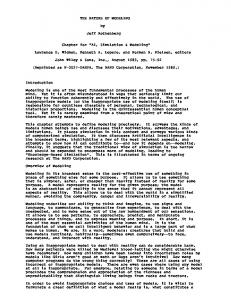
Schematic of a parallel-plate capacitor with a squeezed fluid. . . . . . . 21

3.1

A schematic drawing of an electrically actuated microplate. . . . . . . . 27

3.2

Variation of the Knudsen number with the cavity pressure of the experimental data of Legtenberg and Tilmans (1994). . . . . . . . . . . . . . . 35

3.3

Variation of the squeeze number with the cavity pressure of the experimental data of Legtenberg and Tilmans (1994). . . . . . . . . . . . . . . 36

3.4

Variation of the dimensional fundamental natural frequency of a 210µm length resonator with the cavity pressure. . . . . . . . . . . . . . . . . . 37

3.5

A comparison of the calculated quality factors using the direct numerical approach (stars) and using the perturbation approach (circles) with the experimental data (triangles) of Legtenberg and Tilmans (1994). . . . . 37

4.1

Electrically actuated microplate under the effect of squeeze-film damping. 39

4.2

Variation of the calculated nondimensional fundamental natural frequency for a microplate of length 310µm with the encapsulation pressure. 47

4.3

Comparison of the calculated quality factor (stars) for a microplate of length 310µm to the experimental data (triangles) of Legtenberg and Tilmans (1994). . . . . . . . . . . . . . . . . . . . . . . . . . . . . . . . . 48

4.4

The first mode shape of a microplate of length 310µm. . . . . . . . . . . 49

4.5

The pressure distribution associated with the first mode shape of Figure 4.4. . . . . . . . . . . . . . . . . . . . . . . . . . . . . . . . . . . . . . . . 50

x

4.6

Comparison of the calculated quality factor (stars) for a microplate of length 210µm to the experimental data (triangles) of Legtenberg and Tilmans (1994). . . . . . . . . . . . . . . . . . . . . . . . . . . . . . . . . 51

4.7

The first five mode shapes of a microplate of length 210µm. . . . . . . . 52

4.8

The first five pressure mode shapes corresponding to the deflection mode shapes of Figure 4.7. . . . . . . . . . . . . . . . . . . . . . . . . . . . . . 53

4.9

Comparison of the calculated fundamental natural frequencies and quality factors of a fully clamped microplate (stars) with those of a clampedfree-clamped-free plate (circles). . . . . . . . . . . . . . . . . . . . . . . . 56

5.1

A schematic for a computationally efficient approach to simulate microplates under the coupled effect of electrostatic, fluidic, and mechanical forces. . . . . . . . . . . . . . . . . . . . . . . . . . . . . . . . . . . . 59

5.2

Electrically actuated microplate. . . . . . . . . . . . . . . . . . . . . . . 59

5.3

A comparison of the normalized fundamental natural frequencies calculated using the 2-D finite-element model (circles) with those obtained theoretically (squares) (Younis et al., 2002; Abdel-Rahman et al., 2002) and experimentally (stars) (Tilmans and Legtenberg, 1994) for a 210µm length microbeam. . . . . . . . . . . . . . . . . . . . . . . . . . . . . . . 71

5.4

A comparison of the quality factors of a microplate calculated using the present model (circles) and a linearized plate model (Nayfeh and Younis, 2004) (squares) with the experimental data (triangles) of Legtenberg and Tilmans (1994). . . . . . . . . . . . . . . . . . . . . . . . . . . . . . 71

5.5

A comparison of the quality factors and natural frequencies of a 210µm length microplate calculated using the present model (circles) and a linearized plate model (Nayfeh and Younis, 2004) (stars) for various values of the DC voltage. . . . . . . . . . . . . . . . . . . . . . . . . . . 73

5.6

Variation of the calculated ω1i and ω1r with Vp for Pa = 0.01mbar (circles), Pa = 1mbar (squares), and Pa = 10mbar (stars). . . . . . . . . 74

5.7

Variations of the quality factor with Vp for Pa = 0.01mbar (circles), Pa = 1mbar (squares), and Pa = 10mbar (stars). . . . . . . . . . . . . . 75 xi

5.8

The spatial variation of W1r when Vp = 6V (discrete points) and Vp = 28V (solid and dashes lines). The data shown in circles and dashed line correspond to Pa = 0.01mbar and the data in stars and solid line correspond to Pa = 2mbar. . . . . . . . . . . . . . . . . . . . . . . . . . 76

5.9

The spatial variation of P1r when Vp = 6V (discrete points) and Vp = 28V (solid and dashes lines). The data shown in circles and dashed line correspond to Pa = 0.01mbar and the data in stars and solid line correspond to Pa = 2mbar. . . . . . . . . . . . . . . . . . . . . . . . . . 77

6.1

Electrically actuated microplate. . . . . . . . . . . . . . . . . . . . . . . 86

6.2

Comparison of the quality factors calculated using the present model (solid line) to those of Lifshitz and Roukes (2000) (stars) and Zener (1937) (circles) for various values of T0 . . . . . . . . . . . . . . . . . . . 91

6.3

Comparison of the quality factors of the first mode calculated using the present model (solid line) to those of Lifshitz and Roukes (2000) (stars) and Zener (1937) (circles) for various values of b. . . . . . . . . . . . . . 92

6.4

Variation of the quality factor of the second mode of a plate for various values of b. . . . . . . . . . . . . . . . . . . . . . . . . . . . . . . . . . . 93

6.5

Variation of the ratio between the quality factor of the beam model (Zener, 1937; Lifshitz and Roukes, 2000) to that of the plate model for various values of ν. . . . . . . . . . . . . . . . . . . . . . . . . . . . . . . 94

6.6

Variation of Q of the first mode of a fully clamped plate with T0 . . . . . 95

6.7

Variation of Q of the first mode of a fully clamped plate with h. . . . . 95

6.8

Variation of Q of the first (circles) and second (stars) modes with various values of . . . . . . . . . . . . . . . . . . . . . . . . . . . . . . . . . . . 96

6.9

Variation of Q of the microplate of Figure 6.3 with N1∗ . . . . . . . . . . 96

6.10 Variation of Q of the microplate of Figure 6.3 with Vp . . . . . . . . . . . 97 7.1

A schematic of an electrically actuated microbeam. . . . . . . . . . . . . 99

7.2

Equilibria of an electrostatically actuated microbeam, solid line: stable, dashed line: unstable. . . . . . . . . . . . . . . . . . . . . . . . . . . . . 102

xii

7.3

Frequency-response curves below the dynamic pull-in instability: VDC = 2V and VAC = 0.01V . . . . . . . . . . . . . . . . . . . . . . . . . . . . . 102

7.4

Variation of the normalized nonlinear resonance frequency with the amplitude of AC loading, solid curve: perturbation approach, stars: global approach. . . . . . . . . . . . . . . . . . . . . . . . . . . . . . . . . . . . 103

7.5

Frequency-response curves showing the onset of the dynamic pull-in. . . 104

7.6

Long-time integration results near the upper saddle-node bifurcation of Figure 7.5. . . . . . . . . . . . . . . . . . . . . . . . . . . . . . . . . . . . 104

7.7

Long-time integration results for the lower saddle-node bifurcation of Figure 7.5 and two different initial velocities. . . . . . . . . . . . . . . . 106

7.8

Force-response curves showing the onset of the dynamic pull-in when Q = 1000. . . . . . . . . . . . . . . . . . . . . . . . . . . . . . . . . . . . 107

7.9

Long-time integration results for the two lower saddle-node bifurcations of Figure 7.8. . . . . . . . . . . . . . . . . . . . . . . . . . . . . . . . . . 108

7.10 Force-response curves for the parameters of Figure 7.8 with Q = 100. . . 109 7.11 Long-time integration results showing the onset of dynamic pull-in. . . . 110 7.12 Long-time integration results for the same parameters of Figures 7.8 and different initial conditions. . . . . . . . . . . . . . . . . . . . . . . . 111 7.13 The stability map, any load above a constant σ line will cause pull-in. . 113 7.14 A force-response curve for a case with a softening-type effective nonlinearity. . . . . . . . . . . . . . . . . . . . . . . . . . . . . . . . . . . . . . 114 8.1

Force-response curves obtained using the global approach (heavy curves) and the perturbation-based approximation (thin curves). . . . . . . . . . 116

8.2

Frequency-response curve when VDC = 1.0V , VAC = 0.2V , and Q = 1000.117

8.3

Frequency-response curve when VDC = 2.0V , VAC = 0.2V , and Q = 1000.118

8.4

Frequency-response curves when VDC = 2.0V , VAC = 0.2V , and Q = 500.118

8.5

Frequency-response curve exhibiting dynamic pull-in. . . . . . . . . . . . 119

8.6

Phase portraits for three points on the upper stable branch of Figure 8.5.120

8.7

Phase portraits for two points on the unstable branch of Figure 8.5. Dashed curves denote unstable orbits. . . . . . . . . . . . . . . . . . . . 121 xiii

8.8

Phase portraits for two points on the lower stable branch of Figure 8.5. 122

8.9

Frequency-response curves when VDC = 2.0V , Q = 1000, and VAC = 0.2V .123

8.10 Frequency-response curve when VDC = 2.0V , Q = 1000, and VAC = 0.1V .123 8.11 Frequency-response curve when VDC = 2.0V , Q = 1000, and VAC = 0.07V . . . . . . . . . . . . . . . . . . . . . . . . . . . . . . . . . . . . . . 124 8.12 Force-response curve exhibiting dynamic pull-in when Q = 1000 and Ω = 47.85. . . . . . . . . . . . . . . . . . . . . . . . . . . . . . . . . . . . 124

xiv

List of Tables 2.1

List of effective viscosity models. The parameter α is the accommodation coefficient (approximately equal one) and Q is a coefficient related to the Poiseuille flow (Yang, 1998). . . . . . . . . . . . . . . . . . . . . . 23

xv

Chapter 1

Introduction 1.1

Background and Motivation

Recently, the emerging technology of microelectromechanical systems (MEMS) has seen dramatic progress in fabricating and testing new devices, creating innovative applications, and proposing novel technologies. The fact that they can be manufactured using existing manufacturing techniques and infrastructure of the semiconductor industry means that they can be produced at low cost and in large volumes, making their commercialization quite attractive. Their light weight, small size, low-energy consumption, and durability make them even more attractive. There are numerous MEMS devices that have been successfully used in diverse areas of engineering and science. Ink jet printer heads, micropumps, projection display arrays, and airbag acceloremeters are just few examples, where MEMS devices have replaced more conventional devices in their class for fractions of the cost. Currently, MEMS devices are being actively developed for a wide spectrum of applications in various aspects of life (Elwenspoek and Wiegerink, 2001). In medical applications, for example, MEMS are being implemented for hearing and seeing aids, dosage and draining systems, and nerves stimulation. In information technology, MEMS paved the way for brilliant possibilities, such as increasing significantly the information storage and realizing CD-players in the size of a coin. Unfortunately, simulation tools of MEMS have not kept up pace with this growth 1

Mohammad I. Younis

Chapter 1. Introduction

2

of technology (Senturia et al., 1997). MEMS devices are still being designed by trial and error. A main reason is the fact that the design process of a MEMS device is a multidisciplinary task, which involves inherent coupled-energy domains, such as fluidic, electrostatic, thermal, and mechanical forces. Hence, simulating a MEMS device requires the use of at least two CAD solvers interacting with each other in an iterative manner (Gillbert et al., 1995; Reuther et al., 1996), which is computationally cumbersome. Therfore, these tools are used to simulate the performance of finished devices, rather than to assist their design in preliminary stages of production. Consequently, there are increasing demands toward reducing the complexity of simulations and developing more efficient CAD tools (Senturia et al., 1997; Wachutka, 2002), which can play an effective rule in the development of this technology and realizing reliable devices of optimal performance with minimal cost. RF MEMS is another fast-growing area that promises breakthrough advances in telecomunications, radar systems, and personal mobiles. RF MEMS refers to (Varadan et al., 2003; Tilmans et al., 2003) the application of MEMS technology to highfrequency circuits (radio frequency (RF), microwave, or millimeter wave). Beside the well-known advantages of microtechnology, RF MEMS offer many attractive features over other conventional RF devices. These include increasing bandwidth, highfrequency operating range, and low-insertion loss. RF MEMS consist of passive components, such as transmission lines and couplers, and active components, such as variable capacitors, tuners, switches, and filters. The interest of this dissertation lies in the second category, namely switches and filters (resonators). Mechanical resonators have been widely used as transducers in mechanical microsensors since the mid eighties (Elwenspoek and Wiegerink, 2001). As the area of RF MEMS exploded remarkably and the demand for filters with high resonance frequency and quality factor increased rapidly, microelectromechanical resonators were proposed in the mid nineties (Varadan et al., 2003; Tilmans et al., 2003) as a feasible alternative to comb-drive filters and other conventional large-size filters (Clark et al., 1997). There are a number of actuation methods that can be used to excite resonators,

Mohammad I. Younis


3

such as thermal, piezoelectric, electromagnetic, and electrostatic mechanisms. Electrostatic actuation is the most preferable and well-established actuation method in MEMS because of its simplicity and high efficiency (Varadan et al., 2003). In RF filters, a microbeam is deflected by a DC bias and then driven to vibrate by an AC harmonic load. The frequency of the AC force can be tuned near the fundamental natural frequency of the microbeam, in which case the actuation is called primary-resonance excitation. Alternatively, the microbeam can be excited at other frequencies, such as near half the fundamental natural frequency (superharmonic excitation) or twice the fundamental natural frequency (subharmonic excitation). Recent research (Jin and Wang, 1998) has shown experimentally that using a superharmonic excitation for resonant sensors increases the signal-to-crosstalk ratio compared to that of a primary-resonance excitation. In this dissertation, we simulate the behavior of microbeams actuated by any of the above methods of excitation. RF MEMS switches are a fast-growing area that gained a great deal of attention in recent years. RF MEMS switches overcome the limitations of conventional switches, such as solid-state switches, and present many attractive features, like low-power consumption, high isolation, and low-insertion loss. Similar to resonators, RF switches rely on a mechanical element, which is actuated typically by DC electrostatic forces, to close or break an electric circuit. Major drawback of these devices are the requirement of high driving voltages and the relatively slow response (Varadan et al., 2003; Tilmans et al., 2003). It is highly desirable to bring the actuation voltage to a level compatible or close to that of the circuit devices and to actuate the switch with a very high speed. However, the state-of-the-art of RF MEMS switches is far from achieving these requirements, which forms a barrier towards the development of this technology.

1.2

Common Phenomena in MEMS

In this section, we present a brief introduction to common phenomena in MEMS, which are found nearly in the majority of MEMS devices. Therefore, a thorough understanding of these phenomena is vital for achieving superior design of MEMS

Mohammad I. Younis


4

devices. These phenomena form the core topic of this dissertation.

1.2.1


Typical MEMS devices employ a parallel-plate capacitor, in which one plate is actuated electrically and its motion is detected by capacitive changes. In order to increase the efficiency of actuation and improve the sensitivity of detection, the distance between the capacitor plates is minimized and the area of the electrode is maximized. Under such conditions, the so-called squeeze-film damping (Senturia, 2000; Nayfeh and Younis, 2004) is pronounced. This phenomenon occurs as a result of the massive movement of the fluid underneath the plate, which is resisted by the viscosity of the fluid. This gives rise to a pressure distribution underneath the plate, which may act as a spring and/or a damping force. Recent studies showed that the damping force dominates the spring force at low frequencies, whereas the spring force dominates the damping force at high frequencies.

1.2.2

Thermoelastic Damping

Thermoelastic damping has been shown recently to be a possible dominant source of intrinsic damping in MEMS. Thermoelastic damping results from the irreversible heat flow generated by the compression and decompression of an oscillating structure. A structure in bending has one side under tension and the other side under compression at a higher temperature. This variation in temperature causes a thermal gradient inside the material of the structure, which adjusts itself to allow for a thermal equilibrium. However, the energy used in this adjustment cannot be restored (irreversible process) even if the structure returns to its original state of zero-bending stress. Hence, thermoelastic damping is also referred to as internal friction. According to (Randall et al., 1939), internal friction is defined as “the capacity of a solid to transform its ordered energy of vibration into disordered internal energy”.

Mohammad I. Younis

1.2.3


5

Pull-In Instability

The electric load acting on a capacitor plate is composed of a DC polarization voltage and an AC voltage. The DC component applies an electrostatic force on the plate, thereby deflecting it to a new equilibrium position, while the AC component vibrates the plate around this equilibrium position. The combined electric load has an upper limit beyond which the mechanical restoring force of the plate can no longer resist its opposing force, thereby leading to a continuous increase in the microstructure deflection and, accordingly, an increase in the electric forces in a positive feedback loop. This behavior continues until a physical contact is made with the stationary electrode. This structural instability phenomenon is known as ‘pull-in,’ (Senturia, 2000) and the critical voltage associated with it is called ‘pull-in voltage.’ A key issue in the design of MEMS resonators is to tune the electric load away from the pull-in instability, which leads to collapse of the structure, and hence a failure in the device. On the other hand, this phenomenon forms the basis of operation for RF MEMS switches, in which the mechanical structure is actuated by a voltage load beyond the pull-in voltage to snap the structure with the fastest speed and minimal time.

1.3

Literature Review

In this section, we summarize the main contributions to model and simulate electrically actuated microstructures in the prepense of any of the three basic phenomena of MEMS of Section 1.2. We also discuss the literature work and address the need to improve and extend the state-of-the-art of MEMS modeling and simulation.

1.3.1


There has been extensive research into the behavior of a microplate moving very close to another surface under the effect of squeeze-film damping. Next, we summarize the main contributions. We begin by summarizing papers, which addressed the need to account for squeeze-

Mohammad I. Younis


6

film damping in the modeling of MEMS devices. Newell (1968) studied the effect of damping on miniaturizing cantilever resonators. He divided the pressure range from vacuum to atmospheric pressure into three regimes. In the first regime, the pressure is low (near vacuum) and the damping is dominated by intrinsic damping. In the second regime, the pressure is higher and air damping is dominant, which is due to momentum transfer during collision of the molecules with the moving structure. In this regime, Newell applied the Christian (1966) model, derived by studying the effect of a moving rigid body on changing the linear momentum of the gas molecules. In the third regime, the pressure is high (near atmospheric) and viscous damping is dominant and independent of pressure. In this regime, Newell derived an expression for damping based on the drop in the pressure in a viscous fluid flowing through a parallel-walled duct. Zook et al. (1992) conducted experiments to measure the quality factors of electrostatic clamped-clamped microbeams encapsulated at low pressure. They calculated the quality factors using both the Christian (1966) model in the molecular regime and the Newell (1968) model in the viscous drag regime. Comparing the calculated quality factors with experimental data, they found large discrepancy. Seidel et al. (1990) designed and modeled a capacitive parallel-plate microaccelerometer using a harmonic oscillator with constant damping coefficient. They found that the theoretically predicted frequency-response curves deviate from those obtained experimentally. They also reported an increase in the resonance frequency with increasing residual pressure in the airgap. Legtenberg and Tilmans (1994) and Gui et al. (1995) conducted experiments to measure the quality factors of electrostatic clamped-clamped microresonators encapsulated at very low pressure. They calculated the quality factors of the resonators based on the kinetic theory of gases in the molecular regime (Gupta, 1990). They found that the theory overestimates the measured quality factors by more than two orders of magnitude. They attributed the discrepancy to the fact that the theory does not account for the presence of another electrode, which is very close to the resonator. Next, we summarize contributions, which modeled squeeze-film damping effects in

Mohammad I. Younis


7

MEMS devices employing rigid plates. We begin with Starr (1990) who modeled a capacitive parallel-plate accelerometer using a linearized Reynolds equation. He assumed incompressible fluid, thereby neglecting the spring effect. This assumption reduces the Reynolds equation to the Possion equation, which can be solved either analytically for simple shapes or numerically (e.g., finite-element packages) for complicated shapes. As an example, Starr used the finite-element package ANSYS to calculate the pressure distribution underneath a plate with a hole. He also derived an exact expression for the damping force of a circular disk and an approximate expression for the damping force of a rectangular plate. Chu et al. (1996) modeled the dynamic behavior of parallel-plate electrostatic actuators using a lumped spring-mass model. They used the expressions of Starr (1990), modified by replacing the initial airgap width by the variable distance between the plates. They compared the theoretical frequency-response curve of a plate to experimental data and found that the simulated maximum amplitude is approximately ten times the measured amplitude. The next group of researchers treated the squeeze-film damping problem using the linearized compressible Reynolds equation. Blech (1983) solved analytically the linearized Reynolds equation in the case of oscillating rigid plates of rectangular and circular shapes with trivial pressure boundary conditions and derived analytical expressions for the spring and damping forces. Andrews et al. (1993) conducted experiments on parallel-plate electrostatic microstructures and simulated their dynamic behavior with a spring-mass-damper model. The spring constant was composed of a structural component extracted from the measured resonance frequency at vacuum and a pressure component calculated from the Blech (1983) model. The damping constant was also calculated from the Blech model. They used curve fitting to extract a value for the airgap width. However, they could not obtain a single value for the width that leads to good agreement with the experimental measurements over the entire frequency range, the estimated gap width was 2.1 µm at low frequencies and 1.8 µm at high frequencies. Veijola et al. (1995) investigated the behavior of a capacitive accelerometer, which employs a proof mass supported by a cantilever beam. They simulated its dynamic behavior with a spring-mass-damper model with a parallel-plate electrostatic force. The

Mohammad I. Younis


8

damping coefficient was calculated using the Blech (1983) model and the spring constant was estimated by curve fitting the experimental measurements. They accounted for the slip-flow condition by using an effective viscosity coefficient. They compared their simulations with experimental data and found good agreement. Darling et al. (1998) overcame the limitation of the Blech (1983) model, which was derived only for trivial pressure boundary conditions, by solving the linearized compressible Reynolds equation for arbitrary venting conditions in the case of rigid plates. Their solution scheme is based on Green’s function. The next category of researchers used statistical thermodynamics (Gupta, 1990) to model energy dissipation. K` ad` ar et al. (1996) and Li et al. (1999) modified the Christian model (Christian, 1966) by improving the distribution function of the velocity molecules to reflect more the physics of the problem. They compared their theoretical results to the theory and experimental data of Zook et al. (1992) and found that their theory reduces the discrepancy; however the discrepancy was still significant. Bao et al. (2002) used an energy-transfer model to study the effect of a moving structure on changing the kinetic energy of the gas molecules. They derived an equation for the quality factor, similar to that of Christian (1966), but modified by a correction factor, which is proportional to the gap width and the inverse of the plate length. They compared their theoretical results to the theoretical results and experimental data of Zook et al. (1992) and found that their theory improved the agreement with the experimental data; however there was still significant discrepancy. Next, we summarize models for flexible microstructures. Yang et al. (1997) simulated the dynamic behavior of an electrostatic clamped-clamped microbeam. They used the finite-element package ABAQUS to extract the fundamental free mode shape of the microbeam. They fed this mode shape as a harmonic deflection in the linearized Reynolds equation, modified to account for the slip condition. Then they solved the Reynolds equation over time using finite-difference and Rung-Kutta integration codes. From the results, they extracted effective damping and spring coefficients to be used in a spring-mass-damper model. Then, they calculated the quality factors and the resonance frequencies of two microbeams and compared the results with experiments.

Mohammad I. Younis


9

They found good agreement for the resonance frequencies. They improved the model by lowering the modal stiffness in the simulation to match the experimental data. For the quality factors, they found good agreement up to a pressure value of approximately 1 mbar; below this value, the model overestimated the quality factor. Hung and Senturia (1999) developed a macromodel to simulate the dynamics of a clamped-clamped microbeam proposed as a pressure sensor. They used the Galerkin method to discretize the two coupled partial-differential equations: the Euler-beam equation with the electric and squeeze-film forces and the nonlinear Reynolds equation, modified to account for the slip condition. The global basis functions were extracted using data produced from a few runs of a fully meshed and slow finite-difference method. They indicated that the basis functions of the deflected beam are similar to the linear mode shapes of an undeflected microbeam. On the other hand, they noted that the pressure basis functions exhibit a higher spatial distribution towards the middle of the beam. They computed the time that an undeflected microbeam takes to reach pull-in (the pull-in time) using two models: the macromodel and a model that assumes a linear damping. The results of the two models were then compared to experimental data and results obtained from a full slow finite-difference simulation. The model based on linear damping gave poor results, whereas the macromodel gave results in good agreement with the finite-difference results and experimental data. McCarthy et al. (2002) studied the dynamic behavior of an electrostatic cantilever microswitch. They used a finite-difference scheme to solve two coupled equations: the Euler-beam equation with electrostatic forcing and the compressible Reynolds equation, modified to account for the slip condition. They represented the pressure by the product of an assumed parabolic function along the beam width and an unknown function along the beam length, which is determined in the solution procedure. They integrated the Reynolds equation across the beam width to transform it to a onedimensional equation. They simulated the transient behavior of the beam, compared it to the experimental results, and found good agreement. From the aforementioned review, we note the lack of computationally efficient tools to simulate accurately the dynamic behavior of flexible microstructures in coupled-

Mohammad I. Younis


10

energy fields. The majority of the models treat the microplate as a rigid structure. The few models that account for flexibility of the microstructures have two major shortcomings. First, they approximate the structural problem while solving the flow problem and vice versa, despite the fact that both problems are coupled. Second, they solve the two-dimensional Reynolds equation coupled with a one-dimensional beam equation, in which case the pressure variation across the beam width is neglected (no wrinkles are allowed across the beam). Therefore, these models might not capture accurately the dynamic characteristics of microstructures and might result in inaccurate predictions of the quality factors. Some models require many iterations between different energy-domain finite-element or finite-difference solvers, making the simulation process cumbersome and time consuming. Further, no model has been presented, for this class of coupled problems, to calculate the plate mode shapes, their natural frequencies, and quality factors, while sweeping the DC voltages up to the pull-in instability. Such problems are of significant importance for many MEMS applications, such as MEMS-based projection displays and RF microswitches, in which a microstructure is electrostatically actuated beyond the pull-in instability under the effect of squeeze-film damping to diffract or reflect incident light in the case of displays (Senturia, 2000) or for connecting or breaking an electric circuit for the cases of microswitches (Varadan et al., 2003).

1.3.2


The first to realize the importance of thermoelastic damping and analyze it rigorously is Zener (1937), who gave an analytical approximation for the quality factors of metallic beams due to thermoelastic damping. Roszhart (1990) showed experimentally that thermoelastic damping can limit the quality factors of devices in the micro scale. He used the Zener (1937) model to calculate the quality factors of solid-state resonators and found good agreement with the measurements. Other experimental works showing thermoelastic damping as a dominant source of energy loss in MEMS are also reported by (Evoy et al., 2000) (Duwel et al., 2003). In a recent work, Lifshitz and Roukes (2000) solved exactly the problem of ther-

Mohammad I. Younis


11

moelastic damping of beams and derived an analytical expression for the quality factors. They calculated the quality factors of various microbeams and found that their model yields results close to that of the Zener (1937) model. Microplates have been increasingly tested and used in various MEMS application, such as micropumps and pressure sensors. While the models of Lifshitz and Roukes (2000) and Zener (1937) have been proven to yield quantitatively good results for microbeams, their ability to predict thermoelastic damping in microplates remains questionable. This is particularly important in cases, such as fully-clamped plates, where a beam model does not apply. Also the models of (Lifshitz and Roukes, 2000) and (Zener, 1937) cannot predict the quality factors of structural modes, which vary spatially across the plate width, and hence cannot be captured using a beam model.

1.3.3

The Pull-in Phenomenon and the Behavior of Electrically Actuated Microbeams

Many models have been presented to model the pull-in phenomenon and the static and dynamic behavior of electrically actuated microbeams. An extensive review of these models is summarized in (Younis, 2001). Here, we summarize the major contributions. Then, we review studies addressing the behavior of electrically actuated microbeams and the so-called dynamic pull-in, which is one of the foci of this dissertation. Younis et al. (2002) and Abdel-Rahman et al. (2002) presented a nonlinear model of electrically actuated microbeams, accounting for electrostatic forcing of the air gap capacitor, the restoring force of the microbeam, mid-plane stretching, and an axial load applied to the microbeam. They solved numerically the boundary-value problem describing the static deflection of the microbeam under the DC electrostatic forces using a shooting method. Using a similar procedure, they solved numerically the eigenvalue problem describing the vibration of the microbeam around its statically deflected position for the natural frequencies and mode shapes. Their results show that failure to account for mid-plane stretching in the microbeam restoring force leads to an underestimation of the pull-in instability limit. The results also show that the ratio of the width of the air gap to the microbeam thickness can be tuned to extend

Mohammad I. Younis


12

the domain of the linear relationship between the DC polarization voltage and the fundamental natural frequency. Younis and Nayfeh (2003) expanded on the work of Younis et al. (2002) and AbdelRahman et al. (2002) by considering the microbeam response to a general electric load composed of both DC and AC components. They applied a perturbation method, the method of multiple scales, to the general equation of motion of the microbeam and its associated boundary conditions, and obtained an approximation of the response of the microbeam to a primary-resonance excitation. They derived equations that describe the nonlinear resonance frequency, the amplitudes of periodic solutions, and the stability of these solutions. Their results show that increasing the axial force improves the linear characteristics of the resonance frequency while increasing the mid-plane stretching has the reverse effect. Moreover, the DC electrostatic load was found to affect the qualitative and quantitative nature of the frequency-response curves, resulting in either a softening or a hardening behavior. Finally, they investigated the possibility of activating a three-to-one internal resonance between the first and second modes and found that this kind of nonlinear interaction cannot be activated. Abdel-Rahman and Nayfeh (2003) investigated the response of electrically actuated microbeams to a superharmonic and subharmonic excitations. They used the method of multiple scales to obtain two first-order nonlinear ordinary-differential equations that describe the modulation of the amplitude and phase of the response and its stability. They presented typical frequency-response and force-response curves, exhibiting the coexistence of multivalued solutions. They found that the solution corresponding to a superharmonic excitation consists of three branches, which meet at two saddle-node bifurcation points. On the other hand, the solution corresponding to a subharmonic excitation consists of two branches meeting a branch of trivial solutions at two pitchfork bifurcation points. One of these bifurcation points is supercritical and the other is subcritical. The model of Abdel-Rahman and Nayfeh (2003) applies only for small AC forcing. Younis et al. (2003) and Abdel-Rahman et al. (2003b) developed a reduced-order model to simulate the static and dynamic behaviors of electrically actuated microbeams

Mohammad I. Younis


13

undergoing small or large motions. The model uses few linear undamped mode shapes of a straight microbeam as basis functions in a Galerkin procedure, and hence it reduces the complexity of the simulation and reduces significantly the computational time. Unlike the model of (Younis et al. 2002) and (Abdel-Rahman et al. 2002), the reduced-order model shows high robustness as the pull-in instability is approached. Hence, Younis et al. (2003) and Abdel-Rahman et al. (2003b) utilized the model to study the static behavior of the microbeam more rigorously. They showed that the pull-in voltage corresponds to a saddle-node bifurcation. They calculated the static deflection at each DC voltage and found two solution branches: the larger solution is unstable and the smaller one is stable. As the DC voltage increases, these branches get closer to each other, coalesce, and destroy each other in a saddle-node bifurcation, corresponding to the pull-in voltage. They found that the deflection at pull-in is approximately 57% of the capacitor airgap, which is significantly higher than reported using linear theories, which is ≈ 33%. Finally, they used the model to simulate the dynamic behavior of a MEMS switch and calculate its pull-in time. While the model of (Younis et al. 2003) and (Abdel-Rahman et al. 2003b) allows for a better understanding of the pull-in instability, it is based on static analysis and does not account for the effect of the AC loading. This is particularly important in light of the fact that the behavior of these microelectromechanical systems is nonlinear (Younis et al., 2001; Gui et al., 1998). Therfore, the possibility of a dynamic instability (i.e, ‘dynamic pull-in’) is very high (Nayfeh and Mook, 1979; Nayfeh and Balachandran, 1995; Nayfeh, 2000), which can dangerously take place below the static pull-in voltage (SPV). Unfortunately, no studies have dealt with the effect of the AC loading on the pull-in limit. However, few studies have addressed the dynamic pull-in phenomenon for other kinds of dynamic loadings. Ananthasuresh et al. (1996) and Krylov and Maimon (2003) reported and analyzed the dynamic pull-in for switches actuated by a step voltage with various ramping rates (Ananthasuresh et al., 1996). Both studies (Ananthasuresh et al., 1996; Krylov and Maimon, 2003) indicate that the dynamic pullin voltage can be as low as 91% of the SPV. In the presence of squeeze-film damping, the dynamic pull-in voltage is shown to approach the SPV (Krylov and Maimon, 2003).

Mohammad I. Younis

1.4


14

Dissertation Objectives and Organizations

The objectives of the dissertation are: • To model and simulate accurately the dynamics of microplates under the effect of squeeze-film damping and electrostatic forces and predict their quality factors for various gas pressures and DC loading using the compressible Reynolds equation coupled with a plate model. • To express analytically the pressure distribution underneath a plate in terms of its structural mode shapes using perturbation methods, thereby reducing the dimension of the coupled system and hence the number of global variables required for the simulation. • To study the global dynamics of MEMS resonators employing microbeams excited by primary-, superharmonic-, and subharmonic-resonance excitations. To calculate the microbeams resonance frequencies and amplitudes of vibration, and track their dynamic behavior up to the pull-in instability. To analyze the dynamic pull-in phenomenon and present guidelines for the design of MEMS resonators. To compare the simulation results of the global approach to these predicted analytically using the perturbation-based models of Younis and Nayfeh (2003) and Abdel-Rahman and Nayfeh (2003). • To propose a novel RF MEMS switch actuated by a voltage load much lower than the traditionally used voltage. The new actuation method is based on dynamic pull-in. Here, we propose to actuate the switch using a combined DC and AC loading, similar to the actuation method used in MEMS resonators. The AC loading can be tuned by altering its amplitude and frequency to reach the pull-in instability with the lowest driving voltage and fastest response speed. • To model and simulate thermoelastic damping in microplates and derive analytical expressions for their quality factors. The organization of the dissertation is as follows. In Chapter 2, we present a general theoretical background of damping in MEMS. We focus on squeeze-film damp-

Mohammad I. Younis


15

ing and the Reynolds equation (its assumptions, limitations, and modifications). In Chapter 3, we present a model utilizing the nonlinear Euler-Bernoulli beam equation coupled with a one-dimensional Reynolds equation to calculate the quality factors of electrically actuated microbeams under the effect of squeeze-film damping. We solve the eigenvalue problem, extract the quality factor of a resonator, and compare the results to experimental data. We conclude the chapter by remarking that this model is not adequate to capture the effect of the gas pressure underneath a plate and that a two-dimensional model is needed. In Chapter 4, we present a model utilizing a linearized plate equation coupled with the compressible Reynolds equation to simulate the dynamic behavior of microplates (rectangular plates and circular discs) of generic boundary conditions under the effect of squeeze-film damping and small DC loading. We apply perturbation methods to the compressible Reynolds equation to express the pressure distribution in terms of the structural mode shape, which is substituted into a plate equation. The resulting equation is solved using a finite-element method for the natural frequencies, the structural mode shapes, the corresponding pressure distribution, and the quality factors. We validate the model by comparing the calculated quality factors to experimental data. In Chapter 5, we present a model to simulate the dynamics of microplates under the effect of squeeze-film damping and large electrostatic forces using the compressible Reynolds equation coupled with the von K´ armán plate equations. We utilize the beam model of (Younis et al., 2003) to simulate the static behavior of the microplate under the effect of electrostatic forces. We derive analytical expressions for the pressure distribution in terms of the plate mode shapes around the deflected position, and hence eliminate the pressure as a variable in the solution procedure. We substitute the static deflection and the analytical expression of the pressure into the dynamic von K´ arm´ an plate equations and then solve the resulting equations using a finite-element method. We present several results showing the effect of the pressure and the DC electrostatic forcing on the structural mode shapes, the pressure distributions, the natural frequencies, and the quality factors.

Mohammad I. Younis


16

In Chapter 6, we study thermoelastic damping in microplates and derive analytical expressions for their quality factors. We solve the heat equation for the thermal flux across the microplate, in terms of the plate deflection, and hence decouple the thermal equation from the plate equation. Then, we utilize a perturbation method, the method of strained parameters (Nayfeh, 1981), to derive an analytical expression for the quality factors of microplates, of general boundary conditions under electrostatic loading and residual stresses, in terms of their structural mode shapes. For the special case of no electrostatic and in-plane loadings, we derive a simple analytical expression for the quality factor. In Chapter 7, we use the reduced-order model of (Younis et al., 2003) and (AbdelRahman et al., 2003b) to simulate the global dynamic behavior of MEMS resonators excited near their natural frequencies (primary-resonance excitation). Then we propose a novel RF MEMS switch. We utilize a shooting technique (Nayfeh and Balachandran, 1995) and long-time integrations of the equations of motion to predict periodic motions. We compare the simulation results of this approach to these predicted analytically using the model of (Younis and Nayfeh, 2003). We also remark about the dynamic pull-in phenomenon. Then we use the global approach to demonstrate the new actuation method for the proposed switch. In Chapter 8, we extend the analysis of Chapter 7 to secondary-resonance excitations. We simulate the dynamics of microbeams excited near half their fundamental natural frequencies (superharmonic excitation) and twice their fundamental natural frequencies (subharmonic excitation). For the superharmonic case, we present results showing the effect of varying the DC bias, the damping, and the AC excitation amplitude on the frequency-response curves. We show that the dynamic pull-in phenomenon can occur in a superharmonic excitation at an electric load much lower than that predicted based on static analysis. For the subharmonic case, we show that if the magnitude of the AC forcing exceeds the threshold activating the subharmonic resonance, all frequency-response curves will reach pull-in. Finally, in Chapter 9, we present summary and conclusions of the dissertation and conclude with recommendations for future work.

Chapter 2

Damping in MEMS Damping in microelectromechanical systems (MEMS) strongly affects their performance, design, and control. Damping influences the behavior of MEMS in various ways, depending on their design criteria and operating conditions. For instance, in microaccelerometers, high damping (near critical) is desirable to prevent large resonance responses due to external disturbances, which might result in a mechanical or an electrical failure. On the other hand, in resonant sensors, a high quality factor is required for achieving high sensitivity and resolution. Hence, it is essential to understand the damping mechanisms in MEMS devices to optimize their designs.

2.1

Mechanisms of Energy Losses

There are several mechanisms of energy dissipation in MEMS devices (Tilmans et al., 1992). The most common include losses into the surrounding fluid due to acoustic radiation and viscous damping, losses into the structure mounts, and intrinsic damping caused by losses inside the material of the mechanical structure. Each source of energy loss can be described quantitatively in terms of a corresponding quality factor. The overall quality factor QT ot can be expressed in terms of the individual quality factors

17

Mohammad I. Younis

Chapter 2. Damping in MEMS

18

Qj as 1 1 = QT ot Qj

(2.1)

j

Support losses arise from uncanceled shear forces and moments at the end supports, which transfer energy from the vibrating element to the substrate. Support losses can be minimized by building a symmetric resonator so that it vibrates in a balanced way without moving its center of mass (Corman et al., 1997). Support losses can also be minimized by a proper design of the vibrating structure and its mounting mechanism, such as a double-ended tuning fork or a triple beam structure (Tilmans et al., 1992), and to isolate the vibrating element from the mount using a mechanical isolation mechanism. According to Zook et al. (1992), such special designs might introduce complicated modes of motion. Hence, they recommend designing resonators having fundamental natural frequencies much greater than the vibration modes in the supporting structure. Acoustic radiation results from sound waves generated by the movement of the mechanical element in a direction normal to its surface. This mechanism can be significant if the acoustic wavelength is equal to or less than a typical dimension of the mechanical element, which is uncommon in MEMS. Intrinsic losses in single-crystal materials like silicon are very low and their contribution to the total damping is almost negligible compared to extrinsic losses. Hence, among all damping sources, viscous damping is the most significant source of energy loss in MEMS.

2.1.1


Typical MEMS devices employ a parallel-plate capacitor, in which one plate is actuated electrically and its motion is detected by capacitive changes. Examples of such devices are microaccelerometers, microswitches and microrelays, micropumps, resonant sensors, and gyroscopic sensors. In order to increase the efficiency of actuation and improve the sensitivity of detection, the distance between the capacitor plates is minimized and the area of the electrode is maximized. Under such conditions, the

Mohammad I. Younis


19

so-called squeeze-film damping is pronounced. This phenomenon occurs as a result of the massive movement of the fluid underneath the plate, which is resisted by the viscosity of the fluid. This gives rise to a pressure distribution underneath the plate, which may act as a spring and/or a damping force. Recent studies show that the damping force dominates the spring force at low frequencies, whereas the spring force dominates the damping force at high frequencies. Therefore, viscous damping in many MEMS devices corresponds to squeeze-film damping.

2.2

Reynolds Equation

There are at least three approaches in the literature to model squeeze-film damping. The first approach utilizes statistical thermodynamics. It is based on studying the effect of collisions of the moving structure on the individual molecules of the gas, such as their effect in changing the molecules momentum (Christian, 1966) and energy (Bao et al., 2002). The second approach utilizes a simplified form of the Reynolds equation, obtained by assuming incompressible flow (starr, 1990), and hence it neglects the spring effect of the gas pressure. This simplification reduces the equation to a simple Possion equation, which is easier to solve than the original Reynolds equation. The third approach employs the compressible Reynolds equation, which is modified by correction factors to extend its validity over the operating range of MEMS devices. The third approach is more popular because it gives accurate results with high computational efficiency.

2.2.1

Assumptions and Derivation

The derivation of the Reynolds equation is based on a number of assumptions, which are essential to the understanding of its validity and limitations. The following are the most common (Hamrock, 1991; Khonsari and Booser, 2001): 1. The fluid is Newtonian (the shear stress is directly proportional to the velocity). 2. The fluid obeys the ideal gas law.

Mohammad I. Younis


20

3. The inertia and body forces are negligible compared to the viscous and pressure forces. 4. The variation of pressure across the fluid film is negligibly small. 5. The flow is laminar. 6. The width of the gap separating the two plates, where the gas is trapped inside, is very small compared to the lateral extent of the plates. 7. The fluid can be treated as continuum and does not slip at the boundaries. 8. The system is isothermal. Under these assumptions, the Reynolds equation is derived as follows (Hamrock, 1991; Khonsari and Booser, 2001). Without any loss of generality, we consider two parallel rectangular plates (Figure 2.1) separated by a gap of width d. We assume that one plate is moving vertically while the other plate is stationary. The plate has a length and a width b. A simplified form of the Navier-Stokes equations is obtained by an order-of-magnitude analysis, in which higher-order inertia and gravitation terms are dropped from the original equations. Then, the simplified equations are integrated across the gap width to obtain expressions for the fluid velocities. The results are substituted into the continuity equation to yield a primitive form of the Reynolds equation in terms of the pressure and density. Finally, assuming isothermal conditions and ideal gas law, the density is expressed in terms of the pressure, which in turn substituted into the Reynolds equation to obtain the following standard form of Reynolds equation: ∂ ∂x

∂ ∂P ∂H 3 ∂P 3 ∂P H P + H P = 12η H +P ∂x ∂y ∂y ∂t ∂t

(2.2)

Here, x and y are the positions along the length and width of the plate, respectively, t is time, H is the varying distance between the two plates, P is the total pressure, and η is the viscosity coefficient of the fluid.

Mohammad I. Younis

Chapter 2. Damping in MEMS l Vertically Moving Plate b

d

21

x

z

Squeezed Fluid Stationary Plate

y

Figure 2.1: Schematic of a parallel-plate capacitor with a squeezed fluid.

2.2.2

Limitations and Correction Factors

In practical MEMS applications, the aforementioned assumptions of the Reynolds equation might not be completely satisfied. In fact, some assumptions are inherently violated in certain designs, making predictions of the Reynolds equation suspect. These violations and their effects have been studied and correction factors have been proposed to enable the use of a modified version of the Reynolds equation. Next, we discuss two violations: the continuum assumption (assumption 7) and the assumption of large dimensions of the plate compared to the width of the gap spacing (assumption 6). Other issues, such as thermoelastic effects (Zook, 1992), the effect of the surface roughness (Veijola et al., 1997; Khonsari and Booser, 2001), and the effect of turbulence flow (Khonsari and Booser, 2001) are less common and will not be addressed here. Continuum-Fluid Consideration The main assumption in equation (2.2) is that the gas in the gap can be treated as a continuum. The validity of this assumption depends on the so-called Knudsen number Kn (Khonsari and Booser, 2001), defined as Kn =

λ H

(2.3)

Mohammad I. Younis


22

where H is the variable distance between the two plates and λ is the molecular mean free path of the gas, which is the distance that a gas particle travels between collisions. The parameter λ is related to the local value of the pressure Pa as λ=

P0 λ0 Pa

(2.4)

where P0 and λ0 are the pressure and molecular mean free path at typical ambient conditions. Based on the Knudsen number, the flow can be divided into four regimes (Li, 2000): continuum flow when Kn < 0.01, slip flow when 0.01 < Kn < 0.1, transitional flow when 0.1 < Kn < 10, and free molecular flow when Kn > 10. In the continuum regime, the fluid is governed by the Navier-Stokes equations (or equivalently the Reynolds equation). Slip flow can be described by modifying the zero-velocity boundary conditions in the derivation of Reynolds equation to account for the slip of the flow at the plates boundaries (Burgdorfer, 1959). The flow in the transitional regime is a more subtle issue that needs special treatment (Beskok and Karniadakis, 1996). In the molecular regime, the intermolecular collisions can be neglected and the fluid is governed by the Boltzmann transportation equation. Many MEMS devices are designed to operate at very low pressure with a very small gap between the capacitor electrodes. Under such conditions, the Knudsen number is closer to the noncontinuum regimes, making the use of the Reynolds equation suspect. Fortunately, recent extensive research has extended the validity of the Reynolds equation to the noncontinuum regimes, thereby enabling description of the flow using a single model. This is achieved by using the so-called ‘effective viscosity coefficient’ ηef f , which depends directly on the Knudsen number. Various models have been proposed for ηef f since the beginning of the 20th century, when Knudsen presented a correction coefficient based on his research on the gas flow in capillary tubes (Veijola et al., 1995). His coefficient has been used recently by Andrews et al. (1993) and gave good results. Another well-known correction factor was presented by Burgdorfer (1959). He accounted for the slip flow regime by modifying the boundary conditions to take into account, to the first-order approximation, the slip

Mohammad I. Younis


23

velocities. His modified Reynolds equation has been widely used, examples are found in (Hung and Senturia, 1999) and (McCarthy et al., 2002). However, the Knudsen model is limited to the range 0 < Kn < 1 (Khonsari and Booser, 2001). Thanks to the active research in MEMS, many other models have been proposed in the last two decades. Summary of these models and comparison among some of them are given by (Veijola et al., 1995) and (Li and Hughes, 2000). Here we list these models in Table 2.1. Although all models give close results, the model of Veijola et al. (1995) tends to be more accurate because it is valid over a wider range of Kn . Their model is an empirical approximation of the more complicated expression proposed by Fukui and Kaneko (1988) based on the Boltzmann transport equation. Table 2.1: List of effective viscosity models. The parameter α is the accommodation coefficient (approximately equal one) and Q is a coefficient related to the Poiseuille flow (Yang, 1998).

Knudsen

Author

Year 1906

Burgdorfer Hsia and Domoto

1959 1983

Fukui and Kaneko

1988 1993 1993

Seidel et al. Mitsuya Veijola et al. Andrews and Harris

1995 1995

Effective Viscosity (ηef f ) η

K (K +2.507)

n n 1+ 0.1474(K n +3.095) η 1+6Kn η 2 1+6Kn +6Kn √ π ηD 6Q(D) , D = 2Kn 0.7η 0.7+Kn η 2 1+6 2−α Kn + 38 Kn α η 1.159 1+9.638Kn η 0.9906 1+6.8636Kn

Derived from Gas flow in capillary tubes Navier-Stokes Eqs. + slip flow Experimental data fitting Boltzmann equation Experimental data fitting Navier-Stokes Eqs.+ slip flow Fukui and Kaneko model Experimental data fitting

Finite Size and Edges Considerations In some MEMS devices, the ratio of the gap width to the plate length or width is not sufficiently large, which might violate assumption 6 of Section 2.2.1. In such cases, the Reynolds equation in its original form is inaccurate (Schrag and Wachutka, 2001). Other issues like acoustic radiations and non-developed flow at the edges become important. Schrag and Wachutka (2001) compared results of the damping and spring forces obtained using the Reynolds equation with results obtained using the Navier-

Mohammad I. Younis


24

Stokes-based finite-element program for different ratios of the plate length and width to the gap width. The results show erroneous predictions of the Reynolds equation for ratios 5 and 10, whereas the results are on good agreement for ratio 100. Veijola et al. (2001) compared results of a modified Reynolds equation including acoustic edge effects with results of the original Reynolds equation. They found that the damping force predicted with the modified model is 1.07 and 2.0 of that predicted with the unmodified Reynolds equation when the length-to-gap ratio was 100 and 7, respectively. A similar observation was also reported by Vemuri et al. (2000), who showed that the percentage error in the original Reynolds equation increases with decreasing plate length.

2.3

Intrinsic Damping

Extrinsic damping mechanisms can be minimized by a proper design of devices and their operating conditions. For example, squeeze-film damping can be minimized by increasing the distance between the capacitor electrodes, perforating one of the electrodes, and encapsulating the device at a very low pressure. Support losses also can be minimized by a proper design of the vibrating structure and its mounting mechanism. Intrinsic mechanisms on the other hand are more difficult to control because they depend primarily on the material and geometric properties of the structures. Intrinsic damping increases significantly with minituirization of devices and can limit the quality factors of microstructures in the micro and sub-micro scales. Intrinsic damping in MEMS is still a very active research topic. There are many mechanisms that contribute to intrinsic damping, however the exact contribution of each of them is still unclear. Example of these mechanisms are (Duemling, 2002) phonon-phonon scattering; phonon-phonon-electron scattering; and surface losses, such as losses due to thin film, metal layer, oxide layer, and water layer. There is also energy dissipation due to the relaxation phenomenon. This mechanism is characterized by a peak and a relaxation time (this process is also called Debye relaxation). Examples of this category are thermoelastic relaxation, defect relaxation, and grain-boundary relaxation. Recent studies have shown that thermoelastic damping can be a dominant

Mohammad I. Younis


25

source of intrinsic damping in MEMS.

2.3.1


Thermoelastic damping, also called internal friction, can occur in any material subjected to cyclic stress (Roszhart, 1990). This mechanism becomes a very significant source of energy loss when the period of cyclic stress approaches a structure’s thermal constant. In a thermoelastic solid (Lifshitz and Roukes, 2000), the strain and temperature are coupled through the material thermal expansion coefficient. This coupling provides an energy dissipation mechanism, which allows the system to relax to equilibrium. The relaxation is achieved through the irreversible heat flow across the material of structure with different temperature zones. An example is the case of a structure in bending, in which one of its side is under tension, with cooler temperature, and the other side is under compression, with higher temperature.

Chapter 3

A One-Dimensional Model for Electrically Actuated Microstructures under the Effect of Squeeze-Film Damping In this chapter, we investigate the behavior of electrically actuated microstructures under the effect of squeeze-film damping. Younis (2001) concluded that the nonlinear Euler-Bernoulli beam model can be used to simulate the static and dynamic behavior of a microplate of symmetric boundary conditions and under uniformly distributed electrostatic forces. In this chapter, we extend this model to include the effect of squeeze-film damping using the nonlinear Euler-Bernoulli beam equation coupled with the one-dimensional compressible Reynolds equation. Such a model is very attractive because it is computationally much simpler than a two-dimensional Reynolds equation coupled with a plate equation.

26

Mohammad I. Younis

Chapter 3. One-Dimensional Model l b

v(t)

~

x

h

z

Vp

27

y

Stationary Electrode

Figure 3.1: A schematic drawing of an electrically actuated microplate.

3.1

Problem Formulation

We consider a microplate, Figure 3.1, actuated by an electric load composed of a DC component (polarization voltage) Vp and an AC component ve (t) and subject to a net pressure force P¯ (x, t) per unit area due to the squeeze-film damping effect. Due to the symmetric nature of the electrostatic loading and the plate boundary conditions, we approximate the plate as a beam and write the equation of motion governing its transverse deflection as 2 ∂2w EA ∂w 2 ∂4w ˆ ∂ w dx + N EI 4 + ρbh 2 = ∂x ∂t 2 0 ∂x ∂x2 (Vp + ve (t))2 − P¯ b + 12 0 r b (d − w)2

(3.1)

where x is the position along the microbeam length , w(x, t) is the deflection of the microbeam, t is time, ρ is the material density, h is the microbeam thickness, b is the microbeam width, d is the gap width, A and I are the area and moment of inertia of ˆ is the applied axial force, 0 is the dielectric the cross section, E is Young’s modulus, N constant of vacuum, and r is the relative dielectric constant of the gap medium to an air gap. The last term in equation (3.1) represents the parallel-plate electric force assuming complete overlapping between the area of the microbeam and the stationary electrode. The microbeam is assumed to be clamped at both ends; hence the boundary conditions are w(0, t) = w(, t) = 0,

∂w(, t) ∂w(0, t) = =0 ∂x ∂x

(3.2)

Mohammad I. Younis

Chapter 3. One-Dimensional Model

28

The microbeam deflection under an electric force is composed of a static component due to the DC voltage, denoted by ws (x), and a dynamic component due to the AC voltage, denoted by u(x, t); that is, w(x, t) = ws (x) + u(x, t)

(3.3)

The pressure is generally governed by the two-dimensional Reynolds equation, equation (2.2). Next, we linearize equation (2.2) assuming small-deflection and pressure variations. To this end, we express the variable distance H between the beam and the substrate as H(x, y, t) = d − ws (x) − u(x, t)

(3.4)

and write the total pressure P as P (x, y, t) = Pa + P¯ (x, y, t)

(3.5)

where Pa is the static pressure in the gap. Substituting equations (3.3)-(3.5) into equation (2.2) and retaining the linear terms in the outcome, we obtain the linearized compressible Reynolds equation ∂ ∂ P¯ ∂ P¯ ∂ P¯ ∂u ∂ 3 3 (d − ws ) Pa + (d − ws ) Pa = 12ηef f (d − ws ) − Pa (3.6) ∂x ∂x ∂y ∂y ∂t ∂t where η has been replaced by ηef f , the effective viscosity of the fluid in the gap, to account for the rarefied gas effect through its dependence on the Knudsen number. Here we use the model of Veijola et al. (1995) for ηef f . The pressure boundary conditions are zero flux at the clamped edges of the beam and trivial pressure at the open edges; that is, P¯ (x, 0, t) = P¯ (x, b, t) = 0 ∂ P¯ (, y, t) ∂ P¯ (0, y, t) = =0 ∂x ∂x

(3.7) (3.8)

Mohammad I. Younis


29

Assuming the pressure variation across the beam width is small (i.e., assuming negligible side leakage from the gap spacing), we let the pressure and its gradient in equation (3.6) be independent of y and obtain the linearized one-dimensional Reynolds equation ∂ P¯ ∂ P¯ ∂u ∂ 3 (d − ws ) Pa = 12ηef f (d − ws ) − Pa ∂x ∂x ∂t ∂t

(3.9)

and the boundary conditions are given in equation (3.8). For convenience, we introduce the nondimensional variables (denoted by stars)

where T =

x∗ =

x ,

1

ρbh4 EI

2

t∗ =

t , T

ws∗ =

ws , d

u∗ =

u , d

P¯ P¯ ∗ = Pa

(3.10)

. Substituting equations (3.10) into equations (3.1), (3.2), (3.8),

and (3.9) and dropping the stars, we obtain the following system of coupled nondimensional partial-differential equations: 2 ∂2w ∂4w ∂2w ¯ + α2 [Vp + ve (t)] + = [α Γ(w, w) + N ] − P P 1 non ∂x4 ∂t2 ∂x2 (1 − w)2 ∂w(1, t) ∂w(0, t) = =0 w(0, t) = w(1, t) = 0, ∂x ∂x

¯ ∂ P¯ ∂u ∂ 3 ∂P (1 − ws ) = σ (1 − ws ) − ∂x ∂x ∂t ∂t ¯ ¯ ∂ P (1, t) ∂ P (0, t) = =0 ∂x ∂x where Γ (f1 (x, t), f2 (x, t)) =

1 0

∂f1 ∂f2 dx ∂x ∂x

(3.11a) (3.11b)

(3.12a) (3.12b)

Mohammad I. Younis


30

The nondimensional parameters appearing in equations (3.11) and (3.12) are 2 ˆ 2 12ηef f 2 d N 6 0 r 4 Pa b4 , α2 = , σ = , N= , P = α1 = 6 non h EI Eh3 d3 EId d2 Pa T

(3.13)

The parameter σ is the squeeze number (Senturia, 2000), which represents a measurement of the compressibility of the fluid in the gap. For values of σ near infinity, corresponding to high oscillation frequency, the fluid is trapped in the gap and acts like a spring. For values of σ near zero, corresponding to low oscillation frequency, the fluid is nearly incompressible. To calculate the static deflection of the microbeam, we set the time derivatives and the forcing terms in equation (3.11a) equal to zero and obtain α2 Vp2 d2 ws d4 ws = [α Γ(w , w ) + N ] + 1 s s dx4 dx2 (1 − ws )2

(3.14a)

It follows from equations (3.11b) and (3.3) that the boundary conditions are ws = 0 and

dws = 0 at x = 0 and x = 1 dx

(3.14b)

We generate the problem governing the dynamic behavior of the microbeam around the deflected shape by substituting equation (3.3) into equations (3.11a) and (3.11b) and using equations (3.14) to eliminate the terms representing the equilibrium position. To third-order in u, the result is 2 ∂2u ∂2u ∂4u ¯ + 2α1 Γ (ws , u) d ws + = (α Γ (w , w ) + N ) − P P 1 s s non ∂t2 ∂x4 ∂x2 dx2 2 2 2 2α2 Vp d ws ∂ u + 3 u + α1 Γ (u, u) dx2 + 2α1 Γ (ws , u) ∂x2 (1 − ws ) 3α2 Vp2 2 4α2 Vp2 3 ∂2u + u + α Γ (u, u) + u 1 ∂x2 (1 − ws )5 (1 − ws )4 4α2 Vp 2α2 Vp ve (t)u + · · · + 2 ve (t) + (1 − ws ) (1 − ws )3 ∂u(1, t) ∂u(0, t) = =0 u(0, t) = u(1, t) = 0, ∂x ∂x

(3.15a)

(3.15b)

Mohammad I. Younis


31

where the term involving ve2 (t) is dropped because typically ve2 (t) > 1 in equation (4.25), we use a perturbation technique to express the pressure in terms of the deflection. Then, we substitute this expression into equation (4.24) and solve it using a finite-element method. For large |ωn | σ, the boundary-value problem represented by equations (4.25), (4.28), and (4.31) is a singular-perturbation problem (Nayfeh, 1981). Such a case occurs when the gradient of a dependent variable undergoes rapid changes over a very narrow region. In this problem, the pressure changes sharply near the free edges. We use the method of matched asymptotic expansions (Nayfeh, 1981) to derive a uniform approximation to the solution of equations (4.25), (4.28), and (4.31). In this method, an outer expansion, which is valid everywhere in the domain except near the boundaries, is matched with inner expansions, which are valid only near the boundaries. Then, a composite expansion valid everywhere is formed using the outer and inner expansions. We derive the outer expansion by dividing equation (4.25) by ωn σ, in which case the right-hand side of the resulting equation is very small (O( ), where =

1 ωn σ )

compared to the left-hand side. Hence, the outer solution is given to the first-order

Mohammad I. Younis

Chapter 4. Microplates under Small Electrostatic Forces

44

approximation by ψno = φn

(4.32)

where the superscript o denotes an outer solution. This solution satisfies the boundary conditions (4.31) because φn satisfies similar boundary conditions at x = 0 and 1. However, because ψn = 0 at y = 0 and b/, ψn does not satisfy the boundary conditions (4.28) and hence equation (4.32) is not valid in narrow layers near y = 0 and b/. Therefore, we need to determine two inner expansions valid near these boundaries. We begin by deriving an inner expansion ψni valid in the boundary layer near y = 0. We introduce an inner variable ξ =

y α ,

where α is positive and determined in the course

of the analysis. Next, we rewrite equation (4.25) in terms of ξ and note that α =

1 2

corresponds to the distinguished limit, because it yields the least degenerate form of the resulting equation and allows for a proper matching of the outer and inner solutions (Nayfeh, 1981). Accordingly, we obtain ∂ 2 ψni − iψni = −iφn (x, 0) ∂ξ 2

(4.33)

From equation (4.28), we conclude that ψni (x, 0) = 0

(4.34)

The solution of equation (4.33) that decays away from y = 0 can be expressed as √ ξ − 1+i

ψni (x, y) = φ(x, 0) + c1 e

2

(4.35)

Imposing the boundary condition (4.34), we obtain c1 = −φ(x, 0) To derive an inner solution ψnI near y = b/, we introduce an inner variable η =

b/−y √ ,

Mohammad I. Younis


45

repeat the same previous steps, and obtain √ η − 1+i

ψnI (x, y) = φn (x, b/) − φn (x, b/)e

2

(4.36)

Combining the outer solution, equation (4.32), with the two inner solutions, equations (4.35) and (4.36), we obtain the following general solution, also called composite expansion (Nayfeh, 1981), which is valid everywhere: √ η − 1+i

ψn (x, y) = φn (x, y) − φn (x, b/)e

2

√ ξ − 1+i

− φn (x, 0)e

2

(4.37)

Rewriting equation (4.37) in terms of x and y, we obtain √ − 1+i

ψn (x, y) = φn (x, y) − φn (x, b/)e

2

b/−y √

√ − 1+i

− φn (x, 0)e

2

y √

+ ...

(4.38)

Equation (4.38) gives an approximate analytical expression for the nth complex pressure mode shape in terms of the nth complex plate mode shape and eigenvalue.

4.2

Results

We substitute equation (4.38) into equation (4.24) and obtain b/−y ∂ 4 φn ∂ 4 φn ∂ 2 φn ∂ 4 φn √ √ − 1+i 2 + 2 + − N + P (x, y) − φ (x, b/)e φ non n n 0 0 4 2 2 4 2 ∂x ∂x ∂y ∂y ∂x y √ √ − 1+i − φn0 (x, 0)e 2 − αVp2 φn = ωn2 φn (4.39) Equation (4.39) and the boundary conditions, equations (4.26), (4.27), (4.29), and (4.30) represent a linear distributed-parameter system for the dynamic behavior of the microplate under the coupled effect of squeeze-film damping, the structural forces, and the linear electrostatic forces. We solve this system for the nth complex mode shape and eigenvalue using a finite-element method (Reddy, 1993). We mesh the plate using a ∂w nonconforming rectangular element of four nodes with the three unknowns (w, ∂w ∂x , ∂y )

at each node. We use the Hermite functions as basis functions in the finite-element formulation.

Mohammad I. Younis


46

The real part of the complex eigenvalue gives the natural frequency of the microplate, whereas the imaginary part yields its damping. The quality factor can be related to the imaginary and real parts of the eigenvalue by recalling the relation between the damping coefficient and the quality factor for a spring-damper-mass system; that is, Q=

Re(ωn ) 2Imag(ωn )

(4.40)

where Re and Imag denote the real and imaginary parts, respectively. Next, we calculate the natural frequencies and quality factors of electrically actuated microplates, employed as transducers in resonant sensors, under various gas pressures. We consider first the resonant microplate of Legtenberg and Tilmans (1994) with = 310µm, h = 1.5µm, b = 100µm, d = 1.18µm, E = 166GP a, axial load per unit length of 0.0009 N ewton, and Vp = 2V . The resonator is encapsulated in a cavity at very low pressure. They reported an experimental value of the quality factor near vacuum Qvacuum = 18500 at Pa = 6 × 10−6 mbar. We use this value with equation (2.1) to account for the structural damping of the microplate. In the following figures, we use a mesh of 24 × 8 elements, which yielded acceptable convergence. In Figure 4.2, we show the calculated nondimensional fundamental natural frequency ω10 for various values of the encapsulation pressure Pa . We note that ω10 increases slightly with increasing pressure, an indication of a low spring effect, as expected for this range of pressure. Figure 4.3 shows a comparison of the calculated quality factor Q (stars) to the experimental data (triangles) of Legtenberg and Tilmans (1994). The agreement is excellent except for one data point at Pa = 6 × 10−5 mbar. The reason for this discrepancy is not clear at the present time, especially there is a large drop in the experimental value as Pa increases slightly. More experiments are needed in the interval 10−5 mbar ≤ Pa ≤ 10−1 mbar. Figures 4.4 and 4.5 show the first mode shape of the microplate and the corresponding pressure distribution, respectively, at Pa = 1 mbar. We calculate the mode

Mohammad I. Younis


47

27.1

27

ω1

0

26.9

26.8

26.7

26.6 0

0.5

1

1.5

2

Pa (mbar)

Figure 4.2: Variation of the calculated nondimensional fundamental natural frequency for a microplate of length 310µm with the encapsulation pressure. shape by taking the magnitude of the corresponding complex mode shape, which is in this case dominated by its real part. Next, we consider the resonant microplate of Legtenberg and Tilmans (1994) with length 210µm and Vp = 6V . The reported experimental value of the quality factor near vacuum is Qvacuum = 18000 at Pa = 6 × 10−6 mbar (1994). The rest of the specifications are the same as those of the first microbeam of length 310µm. Figure 4.6 shows a comparison of the calculated quality factor Q (stars) to the experimental data (triangles) of Legtenberg and Tilmans (1994). The agreement is also good. Again, more experiments are needed in the range 10−4 mbar ≤ Pa ≤ 10−1 mbar to better understand the model capability and limitations. Figures 4.7 and 4.8 show the first five mode shapes of the microplate and their corresponding pressure mode shapes, respectively, at Vp = 6V and Pa = 1mbar. The first five natural frequencies are ω10 = 24.21, ω20 = 38.26, ω30 = 63.92, ω40 = 86.35, and ω50 = 118.54. Their corresponding quality factors are Q = 615.94, 1487.70, 5094.20, 5773.10, and 10458.0. For the even modes (antisymmetric modes around y=

b 2 ),

equation (4.38) fails to predict the pressure distribution because the boundary-

layer terms cancel each other. To overcome this problem, we use the symmetry of the

Mohammad I. Younis


48

5

10

4

Q

10

3

10

2

10

1

10 −6 10

−5

10

10

−4

10

−3

10

−2

10

−1

10

0

10

1

Pa (mbar)

Figure 4.3: Comparison of the calculated quality factor (stars) for a microplate of length 310µm to the experimental data (triangles) of Legtenberg and Tilmans (1994). plate about y =

b 2

and simulate half of the plate. The results are then image-mirrored

around the axis of symmetry with a negative sign to take care of the antisymmetry of the mode.

4.3

Other Boundary Conditions

The analysis presented so far is for plates with clamped edges on two opposite sides and free edges on the other sides. Here, we investigate the applicability of the perturbation approach to other boundary conditions. The perturbation approach depends primarily on the fact that ( =

1 σωn0

0 is to be determined later. Next,

we rewrite equation (5.59) in terms of ξ and note that α =

1 2

corresponds to the

distinguished limit (Nayfeh, 1981). Accordingly, we obtain iPni −iWn ∂ 2 Pni − = 2 2 ∂ξ (1 − ws ) (1 − ws )3

(5.71)

From equation (5.64), we conclude that Pni (x, 0) = 0

(5.72)

The solution of equation (5.71) that decays away from y = 0 can be expressed as Pni (x, y) =

ξ Wn (x, 0) √ − 1+i + c1 e 2 1−ws 1 − ws

(5.73)

Imposing the boundary condition (5.72), we obtain c1 = −

Wn (x, 0) 1 − ws

(5.74)

To derive the second inner solution PnI in the boundary layer near y = b/, we introduce an inner variable ζ =

b/−y √ ,

repeat the above steps, and obtain

PnI (x, y) =

ζ Wn (x, b/) Wn (x, b/) − 1+i √ − e 2 1−ws 1 − ws 1 − ws

(5.75)

Combining the outer solution, equation (5.70), with the two inner solutions, equations (5.73) and (5.75), we obtain the following uniformly valid solution, also called composite expansion (Nayfeh, 1981):

Mohammad I. Younis

Pn (x, y) =

Chapter 5. Squeeze-Film Damping and Large DC Forces

70

b/−y 1 √ √ √ √ y − 1+i − 1+i Wn (x, y) − Wn (x, b/)e 2 (1−ws ) − Wn (x, 0)e 2 (1−ws ) 1 − ws (5.76)

By setting ws = 0 in equation (5.76), we end up with an equation similar to that of a plate actuated by small DC forces, which is the case in Chapter 4.

5.4

Results

We solve equations (5.15) and (5.16) using the reduced-order model of Younis et al. (2003) for the static deflection of the microplate under the DC forces. We then substitute the result and equation (5.76) into equation (5.56) and solve the resulting equation along with equations (5.57), (5.58), (5.60-5.63), and (5.65-5.68) using a finite-element method (Reddy, 1993; Zienkiewicz and Taylor, 1991). Details of the derivation of the finite-element model is presented in Section 5.6. The finite-element solution gives the complex eigenvalue ωn and the corresponding eigenvector Wn , Vn , and Un . The real part of ωn yields the nth natural frequency, whereas the ratio between its real and twice its imaginary part yields the quality factor. We use equation (5.76) in the post-processing stage to calculate the pressure distribution underneath the plate. Next, we calculate the natural frequencies and quality factors of electrostatically actuated microplates under the effect of squeeze-film damping. We first consider the microplate designed by Tilmans and Legtenberg (1994) as a resonator, with = 210µm, ˆ = 9.0 × 10− 8N ewton, and b = 100µm, h = 1.5µm, d = 1.18µm, E = 166GP a, N Vp = 6V . We first calculate the damped fundamental natural frequency of the microplate under various DC loadings. We estimate that Pa = 1mbar from matching the calculated Q to the measured value 592 reported by Tilmans and Legtenberg (1994). In Figure 5.3, we show a comparison of the normalized damped fundamental natural frequency ωnor calculated using the present model (circles) with the theoretical results (squares) reported by Younis et al. (2002) and Abdel-Rahman et al. (2002), which are based on

Mohammad I. Younis


71

1

0.9

nor

0.8

ω

0.7

0.6

0.5

0.4

0

5

10

15

20

25

30

Vp (V)

Figure 5.3: A comparison of the normalized fundamental natural frequencies calculated using the 2-D finite-element model (circles) with those obtained theoretically (squares) (Younis et al., 2002; Abdel-Rahman et al., 2002) and experimentally (stars) (Tilmans and Legtenberg, 1994) for a 210µm length microbeam. a beam model, and the experimental data (stars) of Tilmans and Legtenberg (1994). We use a mesh of 24 × 12 in the finite-element program. The agreement between the theoretical and experimental results is excellent, thereby validating the model. 5

10

4

Q

10

3

10

2

10

1

10

−5

10

−4

10

−3

10

−2

10

−1

10

0

10

1

10

2

10

Pa (mbar)

Figure 5.4: A comparison of the quality factors of a microplate calculated using the present model (circles) and a linearized plate model (Nayfeh and Younis, 2004) (squares) with the experimental data (triangles) of Legtenberg and Tilmans (1994). In Figure 5.4, we show a comparison of the calculated quality factors for a mi-

Mohammad I. Younis


72

croplate of length 310µm using the present model (circles) and a linear plate model (Nayfeh and Younis, 2004) derived in Chapter 4 (squares) with the experimental data (triangles) of Legtenberg and Tilmans (1994). The microbeam is actuated at Vp = 2V and its quality factor near vacuum is Qvacuum = 18500. The rest of the specifications are the same as the 210µm microbeam of Figure 5.3. We note that the model gives results very close to the linear model of Chapter 4 because the plates are actuated by low DC voltages, in which the in-plane deflections are negligible. Therfore, we conclude that the simplified linear model of Chapter 4 produces accurate results at low DC loadings. The operating conditions of many MEMS devices exceed the range of small DC loadings. Devices, such as capacitive microswitches and projection arrays, involve large deflections, which can exceed the pull-in instability. In such cases, the in-plane displacements become significant, and hence a simple plate model that neglects the in-plane displacements is suspect. In Figure 5.5, we show a comparison of the calculated quality factors and fundamental natural frequencies of the 210µm microplate of Figure 5.2 using the present model with those calculated using the simplified model in Chapter 4. We note that the simplified model overestimates the quality factors and the natural frequencies at nearly 30% of the pull-in voltage. This is because, as the DC force increases, the static deflection increases, the gap width decreases, and hence the squeeze-film damping increases. Further, the increase in the electrostatic force decreases the natural frequencies. This effect is not represented correctly in the simplified model. We conclude from Figure 5.5a that the use of a single value for the quality factor in the simulation of microdevices involving large bending is inaccurate because it is a strong function of the DC voltage. Next, we investigate the effect of the DC loading and the gap pressure on the natural frequencies, quality factors, mode shapes, and pressure distribution. We consider the microplate of Figure 5.5. Figure 5.6 shows variation of the real part of ω1 (i.e., ω1r ), which yields the fundamental natural frequency, and the imaginary part of ω1 (i.e., ω1i ), which yields the damping of the first mode with Vp for various values of Pa . We note from Figure 5.6a that damping increases with Vp and grows sharply near the

Mohammad I. Younis


73

700

600

500

Q

400

300

200

100

0

0

5

10

15

20

25

30

25

30

Vp (V)

(a) Quality factors.

26 24 22 20

ω1r

18 16 14 12 10 8 0

5

10

15

20

V (V) p

(b) Fundamental natural frequencies.

Figure 5.5: A comparison of the quality factors and natural frequencies of a 210µm length microplate calculated using the present model (circles) and a linearized plate model (Nayfeh and Younis, 2004) (stars) for various values of the DC voltage.

pull-in, where the microplate is highly deflected. Figure 5.6 shows a slight effect of the pressure on ω1r . We conclude from Figure 5.6 that the quality factor, which is the ratio between ω1r and twice ω1i , decreases as Vp increases because of two factors: an increase in the viscous damping due to the decrease in the gap spacing and a decrease in the natural frequency as a result of the negative spring effect of the DC loading.

Mohammad I. Younis


74

Figure 5.7 shows variation of the quality factor with Vp for various values of Pa . 0

10

−1

ω1i

10

−2

10

−3

10

−4

10

0

5

10

15

20

25

30

25

30

Vp (V)

(a) Damping coefficient ω1i .

26 24 22 20

ω1r

18 16 14 12 10 8 0

5

10

15

20

V (V) p

(b) Fundamental natural frequencies ω1r .

Figure 5.6: Variation of the calculated ω1i and ω1r with Vp for Pa = 0.01mbar (circles), Pa = 1mbar (squares), and Pa = 10mbar (stars).

Figure 5.8 shows the spatial variation of the first-mode shape for various values of the electrostatic force and gap pressure. The mode shape is normalized such that its integral over the area of the plate is unity. We note that the pressure has no effect on W1r . The electrostatic force on the other hand influences W1r in the y direction. Figure 5.9 shows the spatial variation of the pressure distribution corresponding to

Mohammad I. Younis


75

5

10

4

10

3

Q

10

2

10

1

10

0

10

0

5

10

15

20

25

30

V (V) p

Figure 5.7: Variations of the quality factor with Vp for Pa = 0.01mbar (circles), Pa = 1mbar (squares), and Pa = 10mbar (stars). Figure 5.8. The function P1r is normalized as W1r . We note that varying the pressure has a slight effect on P1r and that increasing the electrostatic loading has a much significant effect.

5.5

Damping Coefficient for Fully Clamped Microplates

We end up this chapter with the derivation of a damping coefficient, which can be used in reduced-order models, for the case of deflected fully clamped microplates due to large electrostatic forces under the effect of squeeze-film damping. Unlike the case of fixed-free-fixed-free plates, the static deflection ws is a function of x and y. Hence, the calculation of ws (x, y) of fully clamped plates requires the use of a plate model rather than a beam model. One way of achieving this is to use a microplate reduced-order model (Zhao et al., 2004). The structural boundary conditions for fully clamped microplates are Clamped edges at y = 0 and y = b/ Un = Vn = Wn = Wn,x = 0

(5.77)

Mohammad I. Younis


76

0

−0.5

W

1r

−1

−1.5

−2

−2.5 0

0.1

0.2

0.3

0.4

0.5

0.6

0.7

0.8

0.9

1

0.35

0.4

0.45

0.5

x

(a) W1r at y = b/2.

−2.2

−2.25

W1r

−2.3

−2.35

−2.4

−2.45 0

0.05

0.1

0.15

0.2

0.25

0.3

y

(b) W1r at x = 1/2.

Figure 5.8: The spatial variation of W1r when Vp = 6V (discrete points) and Vp = 28V (solid and dashes lines). The data shown in circles and dashed line correspond to Pa = 0.01mbar and the data in stars and solid line correspond to Pa = 2mbar.

Clamped edges at x = 0 and x = 1 Un = Vn = Wn = Wn,x = 0 The pressure boundary conditions are

(5.78)

Mohammad I. Younis


77

0

−0.5

−1

P

1r

−1.5

−2

−2.5

−3

−3.5 0

0.1

0.2

0.3

0.4

0.5

0.6

0.7

0.8

0.9

1

0.35

0.4

0.45

0.5

x

(a) P1r at y = b/2.

0

−0.5

−1

P

1r

−1.5

−2

−2.5

−3

−3.5 0

0.05

0.1

0.15

0.2

0.25

0.3

y

(b) P1r at x = 1/2.

Figure 5.9: The spatial variation of P1r when Vp = 6V (discrete points) and Vp = 28V (solid and dashes lines). The data shown in circles and dashed line correspond to Pa = 0.01mbar and the data in stars and solid line correspond to Pa = 2mbar.

Pn,x (x, 0, t) = Pn,y (x, b/, t) = 0

(5.79)

Pn,x (0, y, t) = Pn,y (1, y, t) = 0

(5.80)

Mohammad I. Younis


78

It follows from equations (5.77-5.80) that there are no boundary layers in this case to the first approximation because the pressure boundary conditions are satisfied to first order according to equation (5.68). To derive an expression for the damping coefficient, we need to proceed to higher orders in the perturbation analysis. To this end, we apply the method of strained parameters (Nayfeh, 1981) and seek a first-order solution to equations (5.56-5.59) and (5.77-5.80) in the form

where =

1 σωn0 .

Wn = Wn0 + Wn1 + ...

(5.81)

Un = Un0 + Un1 + ...

(5.82)

Vn = Vn0 + Vn1 + ...

(5.83)

Pn = Pn0 + Pn1 + ...

(5.84)

ωn = ωn0 + ωn1 + ...

(5.85)

Substituting equations (5.81-5.85) into equations (5.56-5.59) and

(5.77-5.80), we obtain O( 0 ) Wn0 1 − ws L1 (Pn0 , Un0 , Vn0 , Wn0 ) = ∇4 Wn0 − N Wn0 ,xx Pn0 =

(5.86)

2 − α1 Un0 ,x ws,xx − α2 Wn0 ,xx ws,x − α3 Vn0 ,y ws,xx

− α1 us,x Wn,xx − α3 us,x Wn,yy − 2α2 ws,x ws,xxWn,x 2 − α4 Wn0 ,yy ws,x − α5

Vp2 Wn0 + Pnon Pn0 = ωn2 0 Wn0 (1 − ws )3

L2 (Pn0 , Un0 , Vn0 , Wn0 ) = Un0 ,xx + α6 Wn0 ,x ws,xx 1 + α6 ws,x Wn0 ,xx + νVn0 ,xy + (1 − ν)(Un0 ,yy + Vn0 ,xy 2 + α6 ws,x Wn0 ,yy ) = 0

(5.87)

(5.88)

Mohammad I. Younis


L3 (Pn0 , Un0 , Vn0 , Wn0 ) = Vn0 ,yy + νUn0 ,xy 1 + να6 ws,x Wn0 ,xy + (1 − ν)(Un0 ,xy + Vn0 ,xx 2 + α6 ws,x Wn0 ,xy + α6 Wn0 ,y ws,xx ) = 0

79

(5.89)

O( 1 ) ∂ 1 ∂ Wn0 (1 − ws )3 ( Pn1 = ) −i 1 − ws ∂x ∂x 1 − ws ∂ Wn0

∂ (1 − ws )3 ( ) + φ1 + ∂y ∂y 1 − ws

(5.90)

L1 (Pn1 , Un1 , Vn1 , Wn1 ) − ωn2 0 Wn1 = 2ωn0 ωn1 Wn0

(5.91)

L2 (Pn1 , Un1 , Vn1 , Wn1 ) = 0

(5.92)

L3 (Pn1 , Un1 , Vn1 , Wn1 ) = 0

(5.93)

The boundary conditions for equations (5.86-5.93) are At y = 0 and y = b/ Unj = Vnj = Wnj = Wnj ,x = 0

(5.94)

Unj = Vnj = Wnj = Wnj ,x = 0

(5.95)

At x = 0 and x = 1

where j = 0, 1. Substituting equation (5.86) into equation (5.87) and equations (5.86) and (5.90) into equation (5.91), we obtain 2 ∇4 Wn0 − N Wn0 ,xx − α1 Un0 ,x ws,xx − α2 Wn0 ,xx ws,x

− α1 us,x Wn0 ,xx − α3 us,x Wn0 ,yy − 2α2 ws,x ws,xx Wn0 ,x 2 − α3 Vn0 ,y ws,xx − α4 Wn0 ,yy ws,x − α5

+ Pnon

Wn0 − ωn2 0 Wn0 = 0 1 − ws

Vp2 Wn0 (1 − ws )3 (5.96)

Mohammad I. Younis


80

2 ∇4 Wn1 − N Wn1 ,xx − α1 Un1 ,x ws,xx − α2 Wn1 ,xx ws,x

− α1 us,x Wn1 ,xx − α3 us,x Wn1 ,yy − 2α2 ws,x ws,xx Wn1 ,x 2 − α3 Vn1 ,y ws,xx − α4 Wn1 ,yy ws,x − α5

Vp2 Wn1 (1 − ws )3

Wn1 − ωn2 1 Wn0 = 2ωn0 ωn1 Wn0 1 − ws iPnon ∂ ∂ Wn0 (1 − ws )3 ( + ) 1 − ws ∂x ∂x 1 − ws Wn0 ∂ 3 ∂ (1 − ws ) ( ) + ∂y ∂y 1 − ws + Pnon

(5.97)

We note that the homogeneous second-order problem, equations (5.94), (5.95), and (5.97), is the same as the first-order problem, equations (5.94-5.96). Hence, the firstorder problem has a solution only if the right-hand side of equation (5.97) is orthogonal to every solution of the adjoint homogeneous problem governing Wn1 (solvability condition (Nayfeh, 1981)). Noting that the system is self-adjoint, we impose the solvability conditions on equation (5.97) by multiplying its right-hand side with the adjoint of Wn1 and integrating the result over the plate area. The result is 1 b/ Wn0 −iPnon Wn0 ∂ 3 ∂ (1 − w ( ) ) ω1 = 1 b/ s 1 − ws ∂x ∂x 1 − ws 2ωn0 0 0 Wn20 dxdy 0 0 ∂ Wn0 ∂ (1 − ws )3 ( ) dxdy (5.98) + ∂y ∂y 1 − ws Equation (5.98) yields the damping coefficient of the microplate due to squeeze-film damping and large electrostatic forces.

5.6

Finite-Element Formulation

This section gives some details on the finite-element formulation, which is the basis of the finite-element code used in this chapter and Chapter 4.

5.6.1

Weak Form

The first step in generating the finite-element model is to derive the weak form (Reddy, 1993) associated with equations (5.56-5.58), (5.60-5.63), and (5.65-5.68). The weak

Mohammad I. Younis


81

form can be constructed using the principle of virtual displacements. Alternatively, ˆ, we follow Reddy (1993) and multiply equations (5.56-5.58) by the weight functions W ˆ , and Vˆ , respectively, integrate by parts over the area Ωe of an arbitrary element to U distribute the differentiation equally between the weight functions and the dependent variables, and obtain the following weak form:

ˆ ,yy [Wn,yy + νWn,xx] ˆ ,xx [Wn,xx + νWn,yy ] + W W ˆ ,xy Wn,xy + N W ˆ ,x Wn,x − W ˆ α1 Un,x ws,xx + 2(1 − ν)W Ωe

2 2 + α2 ws,x Wn,xx + α3 ws,xx Vn,y + α4 ws,x Wn,yy +

α1 us,x Wn,xx + α3 us,x Wn,yy + 2α2 ws,x ws,xxWn,x + Vp2 W 2 − P F (W , w ) dxdy ωn Wn + α5 non n s (1 − ws )3 ˆ q1 ds + ˆ ,x q2 ds + ˆ ,y q3 ds = 0 W W W + Γe

Γe

(5.99)

Γe

ˆ,y Un,y ˆ,x Un,x + α6 ws,x Wn,x + νVy + 1 (1 − ν)U U 2 Ωe ˆ q4 ds = 0 + Vn,x + α6 ws,x Wn,y dxdy − U

(5.100)

Γe

1

(1 − ν)Vˆ,x Un,y + Vn,x + α6 ws,x Wn,y + Vˆ,y νUn,x Ωe 2 + α6 ws,x Wn,x + Vy dxdy − Vˆ q5 ds = 0 Γe

(5.101)

Mohammad I. Younis


82

where q1 = Wn,xxx + νWn,xyy nx + Wn,yyy + (2 − ν)Wn,xxy ny q2 = − Wn,xx + νWn,yy nx q3 = − Wn,yy + νWn,xx ny 1 q4 = Un,x + α6 ws,x Wn,x + νVy nx + (1 − ν) Un,y 2 + Vn,x + α6 ws,x Wn,y ny 1 q5 = (1 − ν) Un,y + Vn,x + α6 ws,x Wn,y nx 2 + νUn,x + α6 ws,x Wn,x + Vy ny The functional F (Wn , ws ) denotes the right-hand side of equation (5.76), nx and ny are the unit normal vectors of an element boundary Γe , and ds is the arclength of a line element along the boundary.

5.6.2

Finite-Element Model

We use a rectangular element (Reddy, 1993; Zienkiewicz and Taylor, 1991) to discretize the plate. The element has four nodes, with five unknowns (Wn , Wn,x , Wn,y , Un , Vn ) at each node. We express Wn in terms of the Hermite interpolation functions Φj (Reddy, 1993; Zienkiewicz and Taylor, 1991) of a nonconforming rectangular element as

Wn (x, y) =

m

∆ej Φj (x, y),

m = 12

(5.102)

j=1

where the ∆ej are the nodal values of Wn and its derivatives. We use the linear Lagrangian interpolation functions Ψj (Reddy, 1993; Zienkiewicz and Taylor, 1991) to express Un and Vn as Un (x, y) =

n

Uje Ψj (x, y),

n=4

(5.103)

Vje Ψj (x, y),

n=4

(5.104)

j=1

Vn (x, y) =

n j=1

Mohammad I. Younis


83

where the Uje and Vje are the nodal values of Un and Vn , respectively. ˆ = Next, we substitute equations (5.102-5.104) into equations (5.99-5.101), put W ˆ = Ψi , and Vˆ = Ψi , and obtain the following finite-element model for an element Φi , U e: ⎡ −

⎢

⎢ ωn2 ⎢

[0]4×4

⎣ symmetric

⎡

⎫ ⎤⎧ e} ⎪ ⎪ ⎪ ⎪ {∆ ⎪ ⎪ ⎬ ⎥⎨ ⎥ e [0]4×4 ⎥ {U } ⎪ ⎦⎪ ⎪ ⎪ ⎪ ⎪ ⎩ e [0]4×4 {V } ⎭ ⎫ ⎤⎧ e} ⎪ ⎪ ⎪ [K 13 ]12×4 ⎪ {∆ ⎪ ⎬ ⎥⎪ ⎨ ⎥ 23 e [K ]4×4 ⎥ {U } ⎪ ⎦⎪ ⎪ ⎪ ⎪ ⎭ ⎩ {V e } ⎪ [K 33 ]

[M 11 ]12×12 [0]12×4 [0]12×4

[K 11 ]12×12 ⎢ ⎢ + ⎢ K 21 4×12 ⎣ 31 K 4×12 ⎧ ⎪ ⎪ {F 1 }12×1 ⎪ ⎨ = {F 2 }4×1 ⎪ ⎪ ⎪ ⎩ {F 3 } 4×1

[K 12 ]12×4 [K 22 ]4×4 [K 32 ]4×4 ⎫ ⎪ ⎪ ⎪ ⎬

4×4

(5.105)

⎪ ⎪ ⎪ ⎭

where Φi Φj dxdy Mij11 = Ωe 1 Φi q1 + Φi,x q2 + Φi,y q3 ds Fi = Γe Ψi q4 ds Fi2 = Γe 3 Ψi q5 ds Fi =

(5.106) (5.107) (5.108) (5.109)

Γe

Φi,xx [Φj,xx + νΦj,yy ] + Φi,yy [Φj,yy + νΦj,xx] Ωe 2 Φj,xx + 2(1 − ν)Φi,xy Φj,xy + N Φi,x Φj,x − Φi α2 ws,x

11 Kij

=

α1 us,x Φj,xx + α3 us,x Φj,yy + 2α2 ws,x ws,xx Φj,x + 2 Φj,yy + α5 + α4 ws,x

Vp2 Φj − P F (Φ , w ) dxdy non j s (1 − ws )3

(5.110)

Mohammad I. Younis 12 Kij


84

= −α1

Ωe

ws,xx Φi Ψj,x dxdy

(5.111)

13 = −α3 ws,xx Φi Ψj,y dxdy Kij Ωe 1 21 ws,x Ψi,x Φj,x + (1 − ν)ws,x Ψi,y Φj,y dxdy Kij = α6 2 Ωe 1 22 = Ψi,x Ψj,x + (1 − ν)Ψi,y Ψj,y dxdy Kij 2 Ωe 1 23 = νΨi,x Ψj,y + (1 − ν)Ψi,y Ψj,x dxdy Kij 2 Ωe 1 31 = α6 ws,x Ψi,y Φj,x + (1 − ν)ws,x Ψi,y Φj,x dxdy Kij 2 Ωe 1 32 = νΨi,y Ψj,x + (1 − ν)Ψi,x Ψj,y dxdy Kij 2 Ωe 1 33 = Ψi,y Ψj,y + (1 − ν)Ψi,x Ψj,x dxdy Kij 2 Ωe

{∆e } =

Wn1 Wn1 ,x Wn1 ,y ... Wn4 ,y T {U e } = Un1 Un2 Un3 Un4 T {V e } = Vn1 Vn2 Vn3 Vn4

T

(5.112) (5.113) (5.114) (5.115) (5.116) (5.117) (5.118)

(5.119) (5.120) (5.121)

Chapter 6

A Model for Thermoelastic Damping in Microplates In the absence of squeeze-film damping, other energy losses limit the quality factors of microplates. The majority of these losses are extrinsic, and hence can be minimized by a proper design of devices. Thermoelastic damping however is an intrinsic source of energy dissipation, which can affect the quality factor significantly. Thermoelastic damping has been shown recently to be a dominant source of intrinsic damping in MEMS. Thermoelastic damping results from the irreversible heat flow generated by the compression and decompression of an oscillating structure. In this chapter, we present a model and analytical expressions for the quality factors of microplates due to thermoelastic damping. We solve the heat equation for the thermal flow across the microplate, and hence decouple the thermal equation from the plate equation. We utilize a perturbation method to derive an analytical expression for the quality factor of microplates, of general boundary conditions, under electrostatic loading and residual stresses in terms of their structural mode shapes. For the special case of no electrostatic and in-plane loadings, we derive a simple analytical expression for the quality factor, which is independent of the mode shapes. We verify the model by specializing it to a microbeam and comparing the resulting quality factor to that obtained using microbeam models in the literature. We present several results

85

Mohammad I. Younis Chapter 6. A Model for Thermoelastic Damping in Microplates 86 l z Vp+v(t)

Microplate

x b

h y

Stationary Electrode

d

Figure 6.1: Electrically actuated microplate. for various modes of microplates with various boundary conditions.

6.1

Problem Formulation

We consider a microplate (Figure 6.1) actuated by an electric load composed of a DC component Vp and an AC component ve (t). We assume that all forms of extrinsic damping, such as viscous damping, can be neglected. Assuming small strains and displacements, we obtain the following linear equation of motion governing the transverse deflection of the microplate including the effect of thermoelastic damping (Leissa, 1969; Boley and Weiner, 1960): D∇4 w − N1∗

∂2w

Vp ve Vp2 ∂2w + ρh = + 3 w − ∇2 wN T − ∇2 M T ∂x2 ∂t2 d2 d

(6.1)

where w(x, y, t) is the transverse deflection of the plate at the position x and y at time t, ρ is the plate material density, d is the initial gap width, D =

Eh3 12(1−ν 2 )

is the plate

flexural rigidity, h is the microplate thickness, E is Young’s modulus, ν is Poisson’s ratio, N1∗ is the axial force per unit length in the x direction, is the dielectric constant of the gap medium, and N T and M T are the thermal in-plane axial force and bending moment, respectively. The operators ∇2 and ∇4 are the Laplacian and biharmonic operators, respectively. The first two terms on the right-hand side of equation (6.1) represent an approximation of the parallel-plate electrostatic forces assuming a small DC loading and complete overlapping of the microplate and the stationary electrode.

Mohammad I. Younis Chapter 6. A Model for Thermoelastic Damping in Microplates 87 The thermal axial force and bending moment are defined as h/2 Eαt (T − T0 )dz N = 1 − ν −h/2 h/2 Eαt z(T − T0 )dz MT = 1 − ν −h/2 T

(6.2) (6.3)

where T (x, y, z, t) is the temperature distribution, T0 is the stress-free temperature, and αt is the coefficient of thermal expansion. The temperature distribution is governed by the heat conduction equation (Boley and Weiner, 1960) k∇2 T + q = ρCp

Eαt T ∂e ∂T + ∂t 1 − 2ν ∂t

(6.4)

where Cp is the heat capacity coefficient at constant pressure, q is the heat flux, and e is the dilatation strain due to the thermal effect defined as (Boley and Weiner, 1960) e=−

1+ν 1 − 2ν z∇2 w + αt (T − T0 ) 1−ν 1−ν

(6.5)

In most application, T on the right-hand side of equation (6.4) can be replaced by T0 to yield a linear equation for the temperature. Substituting equation (6.5) into equation (6.4) results in the following linearized version of the heat equation: 2

k∇ T + q =

6.1.1

Eα2t T0 (1 + ν) ρCp + (1 − 2ν)(1 − ν)

Eαt T0 ∂ ∂T − (z∇2 w) ∂t 1 − ν ∂t

(6.6)

Linear Eigenvalue Problem

For the linear damped eigenvalue problem, we let w(x, y, t) = φn (x, y)eiωn t

(6.7)

T (x, y, z, t) − T0 = θn (x, y, z)eiωn t

(6.8)

where φn (x, y) and θn (x, y, z) are the nth complex mode shapes of the plate and the associated temperature variation, respectively, and ωn is the nth complex eigenvalue.

Mohammad I. Younis Chapter 6. A Model for Thermoelastic Damping in Microplates 88 Substituting equations (6.7) and (6.8) into equations (6.1) and (6.6), dropping q and the forcing term ve , and noting that the temperature variation across the plate thickness is much larger than its variation across the plane of the plate, we obtain 4

∇ φn − −

k

2φ n ∂x2

∂ N1∗

Eαt 2 ∇ φn + 1−ν

h/2

Eαt θn dz + 1−ν −h/2

h/2

−h/2

z∇2 θn dz

Vp2 φn = ωn2 φn d3

(6.9)

Eα2t (1 + ν)T0 Eαt T0 2 ∂ 2 θn θn − iωn z∇ φn = iω + ρC n p 2 ∂z (1 − ν)(1 − 2ν) 1−ν

(6.10)

The temperature conditions are zero-heat flux from the plate to the ambient (Zener, 1937); that is, ∂θn =0 ∂z

at

1 z= h 2

and

1 z=− h 2

(6.11)

The general solution of equation (6.10) can be expressed as θn =

Eαt T0 z∇2 φn + c1 sin(Kp z) + c2 cos(Kp z) (1 − ν)χ

(6.12)

where Eα2t (1 + ν)T0 , χ = ρCp + (1 − ν)(1 − 2ν)

( ωn χ Kp = (1 − i) 2k

Next, we impose the boundary conditions, equation (6.11), on equation (6.12) and obtain Eαt T0 2 ∇ φn θn = (1 − ν)χ

)

sin(Kp z) z− Kp cos( 12 Kp h)

* (6.13)

Substituting equation (6.13) into equation (6.9), carrying out the integrations, and

Mohammad I. Younis Chapter 6. A Model for Thermoelastic Damping in Microplates 89 retaining the linear terms, we obtain DT ∇4 φn − N1∗

∂ 2 φn Vp2 − 3 φn = ωn2 φn ∂x2 d

(6.14)

where D T = D + Dt and Dt is given by Dt =

h E 2 α2t T0 h3 2 tan(Kp h/2)

+ − (1 − ν)2 χ 12 Kp2 Kp3

(6.15)

Equations (6.14) and (6.15) can be used, along with any appropriate set of boundary conditions, to simulate the behavior of an electrostatically actuated microplate accounting for thermoelastic damping.

6.1.2

Perturbation Analysis

Next, we derive an analytical expression for the quality factors of microplates due to thermoelastic damping. Because Dt