Modeling complex wells with the multi-scale finite ... - Infoscience - EPFL

Journal of Computational Physics 228 (2009) 687–702

Contents lists available at ScienceDirect

Journal of Computational Physics journal homepage: www.elsevier.com/locate/jcp

Modeling complex wells with the multi-scale finite-volume method Patrick Jenny a,*, Ivan Lunati b a b

Institute of Fluid Dynamics, ETH Zurich, ETH-Center, Sonneggstrasse 3, CH-8092 Zurich, Switzerland Laboratory of Environmental Fluid Mechanics, School of Architecture, Civil and Environmental Engineering, École Polytechnique Fédérale de Lausanne, Switzerland

a r t i c l e

i n f o

Article history: Received 23 January 2008 Received in revised form 26 August 2008 Accepted 21 September 2008 Available online 17 October 2008

Keywords: Porous media Multi-phase flow Heterogeneous media Multi-scale finite-volume Well modeling Gravity

a b s t r a c t In this paper, an extension of the multi-scale finite-volume (MSFV) method is devised, which allows to simulate flow and transport in reservoirs with complex well configurations. The new framework fits nicely into the data structure of the original MSFV method and has the important property that large patches covering the whole well are not required. For each well, an additional degree of freedom is introduced. While the treatment of pressure-constraint wells is trivial (the well-bore reference pressure is explicitly specified), additional equations have to be solved to obtain the unknown well-bore pressure of rate-constraint wells. Numerical simulations of test cases with multiple complex wells demonstrate the ability of the new algorithm to capture the interference between the various wells and the reservoir accurately. ! 2008 Elsevier Inc. All rights reserved.

1. Introduction Accurate modeling of subsurface flow is important for many human activities such as sustainable water management; groundwater pollution control and remediation; exploitation of hydrocarbon reservoirs; and CO2 sequestration. Simulations of flow and transport in geological porous media, such as aquifer and oil-gas reservoirs, involve solutions of large problems in complex heterogeneous domains. For example, the most important parameter determining the flow, i.e. the permeability k, usually displays a high degree of variability and is characterized by a hierarchy of heterogeneity scales. In general, the explicit description of this complexity in a traditional simulator is impossible due to the enormous number of degrees of freedom. In this context, multiphase-flow simulations as encountered in reservoir engineering are particularly challenging: the non-linear nature of the problem makes it difficult to obtain accurate results disregarding the fine scale variability of the solution as it is normally done by traditional upscaling techniques. This has led to a flourishing activity in multi-scale modeling, which targets the flow problem with the original resolution by reconstructing the fine-scale details of the solution. Several techniques have been developed which include the multi-scale finite element method (MsFEM) [9], multi-scale mixed finite element methods (MsMFEM) [3,7,2], and the multi-scale finite-volume (MSFV) method [10–12,14,16]. Applications of these techniques to real reservoir problems presuppose the ability of dealing with complex wells that might exhibit complex geometry and penetrate several blocks of the numerical grid. Since the well radius is usually much smaller than the grid-block size, in general wells cannot be modeled explicitly. Due to the essentially singular nature of the well, its pressure (well-bore pressure, pwell ) can significantly differ from the pressure of the grid block perforated by the well (well-block pressure, p). The flux q from the formation into the well is related to these two pressures through the * Corresponding author. Tel.: +41 44 632 6987. E-mail addresses: [email protected] (P. Jenny), [email protected] (I. Lunati). 0021-9991/$ - see front matter ! 2008 Elsevier Inc. All rights reserved. doi:10.1016/j.jcp.2008.09.026

688

P. Jenny, I. Lunati / Journal of Computational Physics 228 (2009) 687–702

productivity index (PI), i.e. q ! PIðp # pwell Þ [18]. For a single-completion well, i.e. a well that penetrates a single grid block, this model corresponds to a Dirichlet boundary condition with p ¼ pwell , if PI ! 1. For a rate-constraint well, q is assigned whereas the well-bore pressure is unknown. A multiple completion well is represented as a line source and the pressure variation in the well-bore (e.g. due to gravity and/or viscous pressure loss) has to be described with an additional equation (well constraint equation). Note that for a rate-constraint well, where the total well rate is specified, the well-bore reference pressure (one single value per well, regardless of the number of completions) appears as an unknown. In the multi-scale finite-element context, well models have been proposed for the MMsFEM [1,3,4] and the MsFEM [8]. Very recently, Krogstad and Durlofsky [13] presented a well model, which accommodates for near well effects and allows a description of well-bore flow. In the framework of the MSFV method, a well model for multiple completions has been proposed by Wolfsteiner et al. [19]. Opposed to the models proposed for MsFEM and MMsFEM, Wolfsteiner et al. account for the extra degree of freedom introduced by the well, which allows solving problems, where only the total well rate is specified and the well-bore reference pressure is an additional unknown (rate-constraint wells). The MSFV method employs an auxiliary coarse grid, together with its dual, to define and solve a coarse-scale pressure problem. The fine scale pressure is approximated by a superimposition of basis functions, which are localized numerical solutions of homogeneous elliptic problems computed on dual cells and are used to interpolate the coarse-grid pressure. When source terms are present (resulting in a non-homogeneous elliptic equation), additional basis functions are needed in order to obtain an accurate pressure approximation. To accomplish this, Wolfsteiner et al. [19] introduced a single basis function per well covering all its completions, i.e. the well basis function is defined on a domain that includes all perforations of that well and overlaps with several dual cells. Since the dual basis functions are unaffected by the presence of the well, two different variables are assigned to the nodes included in the well basis function (split nodes, [19]) in order to guarantee a smooth pressure transition at the boundary of the well basis function. In this paper, an alternative approach to model wells within a MSFV framework is presented. Like in [19] we introduce additional basis functions (well functions) in order to account for the new degrees of freedom represented by the well-bore reference pressures. However, unlike in [19], our well functions have the same support as the original basis functions, i.e. for each well there exists a well function in every dual cell perforated by that well. This enables us to take advantage of the formalism that we have recently developed to model gravity and capillary effects [16] and that can be extended to treat any non-homogeneous elliptic equation (non zero right-hand side) [15]. Note that in the approach presented here, the dual basis functions are modified by the presence of the well. More precisely, the basis functions defined on perforated dual cells are computed by setting the well-bore pressure pwell to zero, which yields a source term of strength q ! PI p. This avoids the introduction of split nodes and allows for a more straightforward pressure reconstruction, even if some coarse cells are perforated by multiple wells. An important advantage of the new multi-scale well modeling approach compared to previous ones is that a regular coarse grid can be applied, as it is shown here for various challenging test cases. These test cases also emphasize the fact that the real challenge is the treatment of line sources (realistic wells) rather than point sources. Especially in the case of rate-constraint wells, where the integral rate of a whole well is specified, an additional unknown (well pressure) appears. Moreover, there is a strong coupling of the reservoir pressure along a well. In the following section, the governing equations are introduced; in Section 3 the MSFV with correction functions is described; in Section 4 one of the most common well models is explained and its integration into the MSFV framework is devised; numerical results are presented in Section 5, where the accuracy of the new MSFV scheme is carefully examined; and conclusions are given in Section 6.

2. Governing equations We consider an incompressible two-phase system, in which the evolution of the phase saturations Sa (a 2 f1; 2g) is described by

/

# ! "$ @Sa @ kr @pa @z ¼ #qa kij a # g qa # @xi @xj @t la @xj

on X:

ð1Þ

Here, as for the rest of the paper, Einstein’s summation convention is employed. By definition, the phase saturations add up to one such that we can use the identity S :¼ S1 ¼ 1 # S2 . The porosity, /, and the permeability tensor, kij , are constant in time, but typically varying in space; the viscosities, la , and the densities, qa , are fluid properties, which we assume constant; kra are the relative permeabilities depending on S; g is the gravitational acceleration; z the depth; and qa source terms due to operating wells. The capillary pressure pc , i.e. the difference between the phase pressures pa , is expressed as an algebraic function of S:

pc ðSÞ ¼ p1 # p2 :

ð2Þ

From now on we use the notation p for p1 , such that the sum of Eq. (1) yields

! " @ @p @r i ¼ kij þq @xi @xj @xi

ð3Þ


689

with

kij ¼kij

! kr 1

þ

kr2

"

ð4Þ

; l l2 # 1 $ @z @p þ f2 c ; r i ¼kij ðf1 q1 þ f2 q2 Þg @xj @xj

ð5Þ

q ¼q1 þ q2 ;

ð6Þ

and

fa ¼

k r a = la ; kr1 =l1 þ kr2 =l2

ð7Þ

which is the fractional flow function of phase a. Note that kij and the right-hand side @ri =@xi þ q depend on the phase saturation S, which evolves as

/

# ! "$ ! " @S @ @z @ @S f1 ui þ kij f2 g Dq Dij þ ¼ # q1 ; @t @xi @xj @xi @xj

ð8Þ

where

ui ¼ ri # kij

@p @xj

ð9Þ

is the total velocity (volumetric flux per unit area),

Dq ¼ q1 # q2

ð10Þ

the density difference and

Dij ¼ kij f1 f2

@pc @S

ð11Þ

the non-linear diffusion coefficient accounting for capillary pressure effects. Note that, together with the algebraic expressions for kra and pc , the elliptic pressure Eq. (3) and the hyperbolic saturation Eq. (8) form a closed system of non-linear PDEs, provided the source terms qa are known. In the following, we explain how this system can be solved with the MSFV method. 3. Basic MSFV Algorithm Solving Eq. (3) may require very high spatial resolution, if the tensor kij or the right-hand side @r i =@xi þ q have complex fine-scale distributions. The aim of the MSFV method is to overcome this resolution gap by reducing the number of coupled degrees of freedom. The MSFV method employees a computational domain that is partitioned by a coarse grid consisting of M control volumes Xk ; k 2 f1; . . . ; Mg (solid lines in Fig. 1). In addition, a dual coarse grid consisting of N control volumes e m ; m 2 f1; . . . ; Ng is required (dashed lines in Fig. 1). Note that the coarse and dual coarse grids can be much coarser than X

xk

Fig. 1. Computational domain X with coarse grid (solid lines) and dual coarse grid (dashed lines); emphasized by bold lines are one coarse control volume X e (dashed). (solid) and one coarse dual control volume X

690


h

h

Φ

Φ

1

1

1

4

4 3

1

~h Ω

2

3

1

~h Ω

2

m Fig. 2. (a) Illustration of basis function Um 1 and (b) illustration of correction function U .

the underlying fine grid representing kij and the right-hand side of Eq. (3). A time step of the solution algorithm can be outlined as follows: ' Sets of basis and correction functions (illustrated in Fig. 2a and b) are computed numerically (some of these may be reused and are updated only periodically based on some adaptivity criterion). !k , which is ' The basis and correction functions are used to construct and solve a problem for the coarse-scale pressure p defined at the dual-grid nodes xk (located within Xk ; see Fig. 1). ' The total velocity u is approximated by the non-conservative fine-scale reconstruction u0 , which is a superposition of basis and correction functions weighted by the corresponding coarse-scale pressure solution. ' The fine-scale solution u0 provides the boundary conditions for local problems, where Eq. (3) is solved within the coarse control volumes Xk in order to obtain a conservative total velocity field u00 . ' The conservative total velocity u00 is used to solve the transport Eq. (8) for S. The original MSFV method [10–12] was not designed to solve elliptic problems with source terms and could not appropriately account for gravity and capillary pressure effects. The reason therefore is that the basis functions and their linear combinations are local solutions of homogeneous (zero right-hand side) elliptic equations. It might seem natural to include the right-hand side into the basis functions directly, but this would yield that the right-hand side scales with the coarse-scale pressures. This led to the idea of introducing correction functions, which are added to the superposition of the basis functions without being multiplied with a coarse-scale pressure value [15–17]. In other words: while the superposition of the basis functions provides a localized homogeneous solution, the correction function is a particular solution. For three-phase flow with gravity it was shown that with correction functions the MSFV solutions are in excellent agreement with the corresponding fine-scale results, while treating gravity only at the coarse-scale leads to large errors. We will see in more detail how the concept of correction functions allows describing effects that are independent of the pressure solution (which is the case for @ri =@xi ). At this point it is assumed that the source term q is known and independent of p. Later, in Section 4, a generalization of the MSFV method for flow scenarios with realistic wells is introduced, where the local rate q depends on both, well- and reservoir pressure. 3.1. Localization and basis functions e m as The basic idea of the MSFV method consists in approximating the fine-scale pressure pðxÞ for x 2 X

pm ðxÞ ¼ Um ðxÞ þ

M X k¼1

! Um k ðxÞpk ;

ð12Þ

m where the basis functions Um k and the correction function U are numerical solutions of

! " @ @ Um k kij ¼ 0 and @xi @xj ! " @ @ Um @r i kij þ q on ¼ @xi @xj @xi

ð13Þ e m; X

ð14Þ

e m , while Um is a parrespectively. Note that the last term in Eq. (12) represents a homogeneous solution of Eq. (3) within X e m . Illustrations of Um and Um are shown in are zero outside the dual volume X ticular solution. By construction, Um and Um k 1 m Fig. 2a and b, respectively. The values at the corners xl of the dual volumes are Um k ðxl Þ ¼ dkl and U ðxl Þ ¼ 0, where dkl is the e m , the conditions Kronecker delta. At @ X


691

! " @ @ Um m~mn m~mi kij k ¼ 0 and @xn @xj

ð15Þ

! " @ @ Um @ % m m & m~mn m~mi kij m~ m~ ri ¼ @xn @xn n i @xj

ð16Þ

! " ! " @ @ Um @ @p em m~mn m~mi kij m~mn m~mi kij ¼ at @ X @xn @xn @xj @xj

ð17Þ

e m pointing outwards, and m ~m is the unit normal vector at @ X ~m ~m are applied, where m n mi is the projector in the direction normal ~ m . This is equivalent to solving a reduced problem to determine the boundary pressure [9]. to @ X Note that differences between MSFV and fine-scale solutions are solely due to this localization, i.e., if

was used as boundary condition, where p is the fine-scale reference pressure, the MSFV and fine-scale solutions would be identical. 3.2. Coarse-scale solution !k , the fine-scale pressure approximation To derive a linear system for the coarse pressure values p

p ( p0 ¼

N X h¼1

M X

Um þ

!l p

l¼1

N X

Um l

h¼1

ð18Þ

is considered. Note that Eq. (18) is a superposition of Eq. (12) and is valid for the whole domain X. With this approximation and applying Gauss’ theorem (or divergence theorem), the integration of Eq. (3) over Xk becomes

Z

kij

@ Xk

@p0 k m! dC ¼ @xj i

Z

Xk

!

" @r i þ q dX; @xi

ð19Þ

where !mk is the unit normal vector at @ Xk pointing outwards. Substituting Eq. (18) for p0 in Eq. (19) leads to Akl

M X l¼1

zfflfflfflfflfflfflfflfflfflfflfflfflZ fflfflfflfflfflfflfflfflffl}|fflfflfflfflfflfflfflfflfflfflfflfflfflfflfflfflfflfflfflfflffl{ XN @ Um l !k ! pl k m dC ¼ ij h¼1 @xj i @ Xk " Z ! XN Z @r i @ Um k þ q dX # kij m! dC; h¼1 @xi @xj i X @X |fflfflfflkfflfflfflfflfflfflfflfflfflfflfflfflfflfflfflfflfflfflfflfflfflfflfflfflfflfflfflfflfflfflfflfflfflfflfflfflfflfflffl{zfflfflfflfflfflfflfflfflfflfflfflfflfflfflfflkfflfflfflfflfflfflfflfflfflfflfflfflfflfflfflfflfflfflfflfflfflfflfflfflfflfflffl}

ð20Þ

Rk

!l and can be written in compact form as which is a linear system for p

! ¼ R: A)p

ð21Þ

Note that the right-hand side Rk consists of two contributions. One is due to the integration of @r i =@xi þ q over the coarse P control volume Xk ; the other, however, is due to the fine-scale flux Nh¼1 kij @ Um =@xj accross the interface @ Xk , hence, it depends on the correction functions. It was demonstrated in a previous paper that this second contribution can be of great importance [16,17]. 3.3. Conservative velocity reconstruction A naive velocity reconstruction based on the superposition (18) yields the volumetric flux

u0i ¼ ri # kij @p0 =@xj ;

ð22Þ

which is (in general) discontinuous across dual volume boundaries. As shown in [10], this leads to severe balance errors when used to solve the saturation Eq. (8). Note, however, that the correct integral balance, i.e. for each coarse volume, is guaranteed by construction. An alternative, conservative reconstruction [10,14] is based on solving the local problems

! " @ @p00 @ri kij þ q on Xk ¼ @xi @xj @xi

ð23Þ

with the boundary conditions

m!ki kij

@p00 @p0 !ki kij ¼m @xj @xj

at @ Xk :

ð24Þ

692


These Neumann boundary conditions guarantee that the fine-scale fluxes are continuous across coarse-cell boundaries and that the integral of the fine-scale fluxes over the boundaries is equal to the sum of the coarse-scale fluxes, hence, that finescale and coarse-scale fluxes are fully consistent. These facts imply that the fine-scale velocity

u00i

¼

(

r i # kij @p00 =@xj r i # kij @p0 =@xj

on Xk at

ð25Þ

@ Xk

is conservative. As discussed in [11], the local reconstruction of the fine-scale velocity u00 , as well as the computation of basis and correction functions, may be done adaptively. Hence, most of the locally computed solutions can be reused for subsequent time steps, even if the global fine-scale pressure field is transient. Since the local problems can be solved independently, the MSFV method is naturally suited for massive parallel computations. The computational efficiency aspects of the algorithm are discussed in [11,12].

4. Well model There exist various ways to describe the interference between wells and reservoir. Here, we consider the common model, in which the local volumetric flow rate of phase a from a well b 2 f1; . . . ; Wg into the reservoir is described as

qba ¼ PIb jkjfa ðpa # pwell;b Þ;

ð26Þ

where we used the definition jkj ¼ kii ðkr1 =l1 þ kr2 =l2 Þ=D (here, D denotes the spatial dimension). The flow rate depends on the difference between the local well-bore and reservoir pressures, pwell;b and pa , respectively, and on the well productivity index PIb [18]. Here, in order to simplify the following derivations, a continuum notation for the productivity index is introduced, where PIb denotes the productivity index per unit segment length along well b. For the computations, the productivity index at the fine grid level is relevant and different than in other multi-scale methods [6], no explicit upscaling thereof is required. Accordingly, the total local volumetric rate from that well is

qb ¼ PIb jkjðp # pwell;b # f2 pc Þ:

ð27Þ

A general approach to compute the local well-bore pressure, pwell;b , is based on solving phase transport equations within the wells with appropriate boundary conditions. Neglecting the viscous pressure loss and assuming that the expected density ref ref hqiwell;b ¼ qref well;b does not vary along the well, pwell;b ðzÞ can be related to the pressure pwell;b at some reference depth zwell;b through ref ref pwell;b ðzÞ ¼ pref well;b þ ðz # zwell;b Þg qwell;b :

ð28Þ

Eq. (28) describes hydrostatic conditions within well b for homogeneous fluid phase distributions and will be used in this paper. However, it is straightforward to employ more general relationships between pwell;b and pref well;b within the same comis putational framework. It is important to distinguish between pressure- and rate-constraint wells. In the first case, pref well;b specified and according to Eqs. (27) and (28), qb ðzÞ can be evaluated directly from the local reservoir pressure p (note that P b q¼ W b¼1 q is the local source term due to all well contributions as it appears on the right-hand side of Eq. (3)). Therefore, the structure of the linear system, which has to be solved to obtain the discretized pressure, is not affected. In the second case, however, the total rate,

qbtot ¼

Z

qb dX;

ð29Þ

X

is specified and pref well;b is part of the solution vector. This leads to an extra equation for each rate-constraint well b, which diwith the reservoir pressure p of each perforated grid cell. Obviously, the linear system, which has to be rectly couples pref well;b solved has a distinctly different structure and is larger than for a reservoir without rate-constraint wells. 4.1. A new well model for the MSFV method e m the e m perforated by well b, a well function Um First, for each well b and each dual volume X well;b is introduced. For x 2 X fine-scale pressure pðxÞ is then approximated as

pðxÞ ( pm ðxÞ ¼ Um ðxÞ þ

M X l¼1

!l Um p l ðxÞ þ

W X b¼1

m pref well;b Uwell;b ðxÞ:

ð30Þ

Note that the last term accounts for the additional degrees of freedom introduced by the wells. Basis, correction, and well functions are numerical solutions of

! " X W @ @ Um l kij PIc jkjUm ¼ l ; @xi @xj c¼1

ð31Þ


! " W @ @ Um @r i X ref kij þ PIc jkj½Um # ðz # zref and ¼ well;c Þg qwell;c # f2 pc + @xi @xj @xi c¼1 m

@ Uwell;b @ kij @xi @xj

!

¼

W X

c¼1

PIc jkjðUm well;b # dbc Þ

693

ð32Þ

ð33Þ

e m with the boundary conditions on X

! " @ @ Um m~mn m~mi kij l ¼0; @xn @xj ! " @ @ Um @ % m m & ¼ m~mn m~mi kij m~ m~ ri and @xn @xn n i @xj ! @ Um @ m~mn m~mi kij well;b ¼0 @xn @xj

ð34Þ ð35Þ ð36Þ

e m , respectively. To derive Eqs. (31)–(33), the pressure p in Eqs. (3) and (27) was substituted by Um , Um and Um , at @ X l well;b respectively. Moreover, to obtain Eqs. (31) and (33), those terms independent of p were omitted and in all three cases the ref well reference pressure values were set to zero except for Eq. (33), where pwell;b was set to one. The localization boundary conditions (34),(35) are the same as for the MSFV method without wells and for the well basis functions the same homogeneous reduced problem boundary conditions are employed as for the basis functions. Note that summing Eqs. (31)–(33) !l , 1 and pref weighted with p well;b , respectively, yields

! " W @ @pm @r i X @r i kij þ PIc jkjðpm # p c # f2 pc Þ ¼ þ q; ¼ @xi @xj @xi c¼1 |fflfflfflfflfflfflfflfflfflfflfflfflfflfflfflfflfflfflfflfflffl {zfflwell; fflfflfflfflfflfflfflfflfflfflfflfflfflfflfflfflfflfflfflffl } @xi

ð37Þ

qc

which shows that superimposing basis-, correction- and well functions is consistent with Eqs. (3), (27) and (28). !l and pref To derive a coarse system for the unknown pressures p well;b , we substitute

p0 ¼

N X h¼1

Um þ

M X

!l p

l¼1

N X h¼1

Um l þ

W X b¼1

pref well;b

N X h¼1

Um well;b ( p

ð38Þ

into Eq. (3) and integrate it over Xk . This leads to M linear equations of the form M X l¼1

!l Akl þ p

W X b¼1

pref well;b Bkb ¼ Rk

ð39Þ

!l and pref for the M þ W unknowns p , where the coefficients are well;b

! N X W Z X @ Um l !k kij mi dC PIc jkjUm l dX; @xj @ Xk Xk h¼1 c¼1

Akl ¼

Z N X

Bkb ¼

N Z X

Rk ¼

h¼1

h¼1

Z

@ Xk

kij @ Xk

Z N X W Z X @ Um well;b k m!i dC PIc jkjUm PIb jkjdX and well;b dX @xj Xk Xk h¼1 c¼1

!ki dC # ri m

N Z X h¼1

kij

@ Xk

N X W Z W Z X @ Um k X ref m!i dC PIc jkjUm dX PIc jkj½#ðz # zref well;c Þg qwell;c # f2 pc +dX: @xj Xk c¼1 Xk h¼1 c¼1

ð40Þ

ð41Þ

ð42Þ

Additional W equations of the form M X l¼1

!l C bl þ p

W X

c¼1

pref well;c Dbc ¼ T b

ð43Þ

are introduced by the well constraints, i.e. from the conditions

qbtot ¼

Z

qb dX

X

ð44Þ

for rate-constraint wells and ref pref well;b ¼ pwell;b ðtÞ

ð45Þ

694


for pressure-constraint wells. Substituting the approximation (30) for p in Eq. (27) leads to the coefficients

C bl ¼ Dbc ¼

Z

X

Z

X

T b ¼qbtot

PIb jkj

N X

þ

X

! N X fUm g # d and bc dX well;c h¼1

"

PIb jkj ðz #

zref well;b Þg

ref well;b

q

#

for rate-constraint wells and

C bl ¼ 0;

ð46Þ

h¼1

PIb jkj Z

Um l dX;

Dbc ¼ dbc

N X h¼1

ð47Þ

#

m

U þ f2 pc dX

ð48Þ

and T b ¼ pref well;b ðtÞ

ð49Þ

!l and the for pressure-constraint wells. Eqs. (39) and (43) form a closed linear system for the M coarse-scale pressure values p , which can be written as W well reference pressures pref well;b

#

A C

$ # ! $ # $ p R : ) ref ¼ p T D well B

ð50Þ

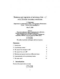
! and pref !l and pref Note that the vectors p consist of the components p , respectively. well well;b 5. Numerical results The numerical simulations are performed on a 2D domain of size Lx , Ly , which is discretized by a fine grid consisting of 220 , 55 cells. The coarse grid used by the MSFV method consists of 20 , 5 cells, which corresponds to an upscaling factor of 11 , 11. Both, homogeneous and heterogeneous permeability fields are considered; the heterogeneous fields have a log-normal distribution and are characterized by an exponential variogram with a correlation length equal to 10 cells. Since the accuracy of the proposed MSFV framework, as that of the original MSFV method, depends on the permeability field, two values are considered for the variance of the log-permeability, i.e. r2ln k ¼ 5:3 and 15.9 (natural logarithm). Moreover, five realizations were generated for each value. No-flow boundary conditions are imposed at the four sides of the domain and the flow is driven by three geometrically complex wells (see Fig. 3), which can be rate or pressure-constraint depending on the flow scenario considered (Table 1). The MSFV results are compared with the corresponding fine-scale reference solutions computed with a standard finitevolume scheme. To solve coupled flow and transport problems, the IMPES (implicit pressure, explicit saturation) approach is employed [5], where a second order upwind scheme is used for transport on the fine-grid.

55 44

A

C

B

33

A.I

22 11 0 0

11

22

33

44

55

66

77

88

99 110 121 132 143 154 165 176 187 198 209 220

Fig. 3. Geometry of the three complex wells used for the numerical test cases: well A (white) is k-Shaped and bifurcates into two branches A and A.I; branch A intersects with well B.

Table 1 Different flow scenarios considered for the numerical simulations. Both, flow-constraint (F) and pressure-constraint (P) wells are used. Scenario

1 2 3

Type

F P P

Well A

Type

pwell

PI

Unknown 0 p- ¼ DqgLy

1 0.1 1

P P P

Well B

Type

pwell

PI

0 0 0

0.1 1 1

P F P

Well C pwell

PI

0 Unknown 0

1 1 1

695


5.1. Single-phase flow

dimensionless rate [–]


First, we consider the scenarios 1 and 2 of Table 1 for one-phase flow (for which gravity and capillary effects can be neglected) in a reservoir with homogeneous permeability k. In scenario 1, the pressure in wells B and C is set to zero, i.e. pwell;B ¼ pwell;C ¼ 0, whereas well A is modeled as a rate-constraint injection well with the total rate qA ¼ qinj and the unknown well-bore pressure pwell;A . In scenario 2, well C is modeled as a rate-constraint well characterized by the total rate qC ¼ qinj and the unknown well-bore pressure pwell;C . The pressure in the other two wells is set to zero. Comparison between the MSFV and fine-scale reference solutions shows that the relative errors of the injection-well f f pressures, i.e. !p ¼ ðpms well # pwell Þ=pwell , are 1.8% and 0.4% for the flow scenarios 1 and 2, respectively. For both scenarios, the dimensionless-rate (q=qinj ) profiles along the three wells are shown in Fig. 4, whereas the dimensionless reservoir pressure in the perforated cells (p=pinj ) is plotted in Fig. 5. The MSFV solution is in good agreement with the reference solution, although in scenario 1 some deviation can be observed in the region close to the intersection of wells A and B (two fine cells are completed by both wells). We attribute this to the strong interference between these two wells, which reduces the quality of the localization assumption. In order to further evaluate the performance of the new multi-scale framework for realistic wells, tracer transport in the velocity field provided by the MSFV method was simulated and the results obtained after 1 PVI (pore volume injected) are compared with the corresponding fine-scale reference solutions. The tracer is injected at constant concentration c0 and there is no tracer in the reservoir initially. Since physical dispersion is neglected and a second order upwind scheme is used for transport, the tracer fronts remain very sharp and can be represented by the concentration contour lines for c=c0 ¼ 0:5,

0.04 A.I

A

0.02 0

–0.04

C

B

–0.02 0

50

100

150

200

250

0.15 A.I

A

0.1 0.05

–0.05

C

B

0 0

50

100

150

200

250

dimensionless p[–]

dimensionless p [–]

Fig. 4. Flow scenarios 1 (top) and 2 (bottom) for single-phase flow and homogeneous permeability. Comparison between the dimensionless rate (q=qinj ) profiles predicted by the MSFV method (circles) and the fine-scale solver (solid lines).

1.5 A.I

A

1

0

C

B

0.5

0

50

100

150

200

250

1 A.I

A 0.5

C

B 0

0

50

100

150

200

250

Fig. 5. Flow scenarios 1 (top) and 2 (bottom) for single-phase flow and homogeneous permeability. Comparison between the dimensionless pressure (p=pinj ) profiles predicted by the MSFV method (circles) and the fine-scale solver (solid lines).

696


which are depicted in Fig. 6 for the flow scenarios 1 and 2. It can be observed that the discrepancy between the MSFV and fine-scale reference solutions, which can be interpreted as a measure of the integral error (over time) introduced by the MSFV approximations, is small in both cases. Notice also that the error near the well intersection point discussed above (see Fig. 4) only has a local effect here. The high accuracy of the MSFV method is also confirmed by the plots shown in Fig. 7, which depict the mass recovery fractions (fraction of recovered fluid, which was initially in the reservoir) as functions of time. Next, the two sets of heterogeneous permeability fields are considered. Although in general the relative well-pressure error !p is larger than in the corresponding homogeneous cases, in both flow scenarios it remains smaller than 10% for r2ln k ¼ 5:3 (Table 2). For r2ln k ¼ 15:9, which is an extremely large variance, the error increases up to approximately 30% for scenario 1 with the permeability realizations 3 and 5. Note, however, that even in these cases the dimensionless rate profiles (no shown here) are in reasonable agreement with the fine-scale reference solutions. Since the quality of the MSFV solutions is similar for the five permeability fields, only the results of realization 1 are shown. In general, the difference between the local well rates computed with the MSFV method and a standard finitevolume scheme is very small (Figs. 8–11). Note also that the artifacts due to the interference between wells A and B are much smaller than in the homogeneous case, mainly due to the dominant influence of the heterogeneity (which is captured efficiently by the MSFV method) on the local well rates. Finally, the plots in Fig. 12 show the mass recovery rates from the MSFV

55 44 33 22 11 0

11

22

33

44

55

66

77

88

99 110 121 132 143 154 165 176 187 198 209 220

0

11

22

33

44

55

66

77

88

99 110 121 132 143 154 165 176 187 198 209 220

5 44 33 22 11

Fig. 6. Flow scenarios 1 (top) and 2 (bottom) for single-phase flow and homogeneous permeability. Comparison between the tracer-front positions predicted by the MSFV method (solid lines) and the fine-scale solver (dashed lines).

0.4

0.45

0.35

0.4 0.35 recovery fraction [–]

recovery fraction [–]

0.3 0.25 0.2 0.15 0.1

0.25 0.2 0.15 0.1

0.05 0

0.3

0.05 0

0.2

0.4 0.6 time [PVI]

0.8

1

0

0

0.2

0.4 0.6 time [PVI]

0.8

1

Fig. 7. Mass recovery fraction (i.e. the fraction of recovered mass initially present in the reservoir) as a function of time for (a) flow scenario 1 and (b) flow scenario 2. Comparison between the MSFV predictions (solid lines) and the fine-scale reference solutions (circles).

697

P. Jenny, I. Lunati / Journal of Computational Physics 228 (2009) 687–702 Table 2 Relative well-bore pressure error

f f !p ¼ ðpms well # pwell Þ=pwell .

2 ln k

r

Real 1 (%)

Real 2 (%)

Real 3 (%)

Real 4 (%)

Real 5 (%)

0.0 5.3 15.9 0.0 5.3 15.9

1.8 #0.51 3.58 0.4 #1.53 #3.74

– 4.70 9.78 – #4.91 11.38

– #0.30 27.02 – #2.61 #4.72

– 1.80 2.91 – 1.86 14.19

– #0.24 30.81 – #9.75 1.59


Scenario 1 1 1 2 2 2

0.1 A.I

A

0.05 0

–0.1

C

B

–0.05 0

50

100

150

200

250


Fig. 8. Flow scenario 1 for single-phase flow and heterogeneous permeability distribution with a variance of r2ln k ¼ 5:3 (realization 1). Comparison between the dimensionless rate (q=qinj ) profiles predicted by the MSFV method (circles) and the fine-scale solver (solid lines).

0.2 A.I

A

0.1 0

–0.2

C

B

–0.1 0

50

100

150

200

250



0.2 A.I

A

0.1 0

–0.2

C

B

–0.1 0

50

100

150

200

250 2 ln k


Fig. 10. Flow scenario 2 for single-phase flow and heterogeneous permeability distribution with a variance of r ¼ 5:3 (realization 1). Comparison between the dimensionless rate (q=qinj ) profiles predicted by the MSFV method (circles) and the fine-scale solver (solid lines).

0.4 A.I

A

0.2 0

–0.4

C

B

–0.2 0

50

100

150

200

250


698

a


b

0.5 0.45

0.35

0.4

1

1

0.3

0.35



0.4

3

0.3 0.25

2

0.2 0.15

0.25 0.2

5 0.15 0.1

0.1

0 0

4 0.2

0.4 0.6 time [PVI]

0

1

0

0.2

4

0.4 0.6 time [PVI]

0.8

1

d 0.45 2

0.3

4

0.4

1

0.35

5

0.25


0.35


0.8

0.4

3

0.2 0.15 0.1

3 1

0.3 0.25

4

0.2

2

0.15

5

0.1

0.05 0

3

0.05

0.05

c

2

5

0.05 0

0.2

0.4

0.6

0.8

1

time [PVI]

0

0

0.2

0.4

0.6

0.8

1

time [PVI]

Fig. 12. Mass recovery fraction (i.e. the fraction of recovered mass initially present in the reservoir) as a function of time for (a) rln k ¼ 5:3 and flow scenario 1, (b) rln k ¼ 15:9 and flow scenario 1, (c) rln k ¼ 5:3 and flow scenario 2, and (d) rln k ¼ 15:9 and flow scenario 2. Comparison between the MSFV predictions (solid lines) and the fine-scale reference solutions (dashed line) for five independent realizations.

55 44 33 22 11 0

0

11

22

33

44

55

66

77

88

99 110 121 132 143 154 165 176 187 198 209 220

Fig. 13. Flow scenario 1 for single-phase flow and heterogeneous permeability distribution with a variance of r2ln k ¼ 5:3 (realization 1). Comparison between the tracer-front positions predicted by the MSFV method (solid lines) and the fine-scale solver (dashed lines).

and fine-scale simulations. Again, the agreement is very good for r2ln k ¼ 5:3 and reasonable for r2ln k ¼ 15:9 for all realizations. Finally, the concentration contour lines for c=c0 ¼ 0:5 of the MSFV and fine-scale solutions are compared in Figs. 13–16 for realization one.


699

55 44 33 22 11 0 0

11

22

33

44

55

66

77

88

99 110 121 132 143 154 165 176 187 198 209 220


55 44 33 22 11 0 0

11

22

33

44

55

66

77

88

99 110 121 132 143 154 165 176 187 198 209 220


55 44 33 22 11 0 0

11

22

33

44

55

66

77

88

99 110 121 132 143 154 165 176 187 198 209 220


Fig. 17. Multi-phase flow with gravity in a homogeneous permeability field; bottom: MSFV solution of water saturation; top: reference fine-scale solution of water saturation.

700


Fig. 18. Multi-phase flow with gravity in a homogeneous permeability field; bottom: MSFV solution of pressure; top: reference fine-scale solution of pressure.

Fig. 19. Permeability field used for the heterogeneous multi-phase flow test case with gravity (r2ln k ¼ 5:3, realization 3).

Fig. 20. Multi-phase flow with gravity in a heterogeneous permeability field (r2ln k ¼ 5:3, realization 3); bottom: MSFV solution of water saturation; top: reference fine-scale solution of water saturation.

5.2. Multiphase flow As an ultimate test of model performance we consider a multiphase-flow problem: the reservoir is initially fully saturated with oil (o), then water (w) is injected at constant pressure in well A, i.e., pwell;A ¼ p- (flow condition 3 in Table 1). Both liquids are assumed incompressible; the relative density difference is Dq=qw ¼ ðqw # qo Þ=qw ¼ 0:5; the viscosity ratio M ¼ lw =lo ¼ 0:1; and the gravity number G ¼ DqgLy =p- ¼ 1. Since the liquids are immiscible, relative permeabilities are modeled as quadratic functions of the phase saturation, i.e., krw ¼ S2w and kro ¼ S2o ¼ ð1 # Sw Þ2 ; capillary pressure is neglected. At a given time, the MSFV solutions for a homogeneous permeability field are compared with the fine-scale reference


701

Fig. 21. Multi-phase flow with gravity in a heterogeneous permeability field (r2ln k ¼ 5:3, realization 3); bottom: MSFV solution of pressure; top: reference fine-scale solution of pressure.

solutions in Figs. 17 and 18. Both saturation and pressure solutions are in good agreement. In Figs. 20 and 21, the results obtained with a heterogeneous permeability field (r2ln k ¼ 5:3, realization 3, Fig. 19) are illustrated. Again, the MSFV solution is in good agreement with the fine-scale solution. 6. Conclusions A new approach that accurately treats complex, interfering wells within the MSFV framework is devised. Opposed to previous models [19], which depend on additional sub-domains each covering a whole well, the same dual coarse grid cells as for the original MSFV method are used as support of the well basis functions. Therefore, the algorithm nicely fits into the data structure of the original MSFV method and does not require solutions of the fine-scale flow problem on larger domains. This is an important requirement in order to maintain the order of the complexity of the MSFV method. Note that here no additional approximations are made, i.e. the quality of the solutions solely depends on the accuracy of the reduced problem boundary conditions. It is shown analytically that this MSFV method for multi-phase flow in heterogeneous media is consistent with corresponding fine-scale methods in the sense that the solutions become identical, if exact localization boundary conditions are applied. Numerical multi-phase flow studies with homogeneous and heterogeneous permeability fields and interfering pressureand rate-constraint wells were performed with and without gravity effects. In all cases the MSFV pressure and saturation solutions are in excellent agreement with the fine-scale simulations. The same can be stated about well pressure- and rate logs and about oil recovery over time. Finally, it was demonstrated that the method also is very accurate for complex multiphase flow and transport problems, which involve strong gravity effects. References [1] J.E. Aarnes, On the use of a mixed multiscale finite elements method for greater flexibility and increased speed or improved accuracy in reservoir simulation, Multiscale Model. Simul. 2 (3) (2004) 421–439. [2] J.E. Aarnes, V. Kippe, K.A. Lie, Mixed multiscale finite elements and streamline methods for reservoir simulation of large geomodel, Adv. Water Res. 28 (2005) 257–271. [3] T. Arbogast, Implementation of a locally conservative numerical subgrid upscaling scheme for two phase darcy flow, Comput. Geosci. 6 (2002) 453– 481. [4] T. Arbogast, S.L. Bryant, Numerical subgrid upscaling for waterflood simulations, in: SPE 66375, Presented at the SPE Symposium on Reservoir Simulation, Houston, February 11–14, 2001. [5] K. Aziz, A. Settari, Petroleum Reservoir Simulation, Applied Science Publ. Ltd., London, UK, 1979. [6] Y. Chen, X.-H. Wu, Upscaled modeling of well singularity for simulating flow in heterogeneous formations, Comput. Geosci. 12 (2008) 29–45. [7] Z. Chen, T.Y. Hou, A mixed finite element method for elliptic problems with rapidly oscillating coefficients, Math. Comput. 72 (242) (2003) 541–576. [8] Z. Chen, X. Yue, Numerical homogenization of well singularities in flow and transport through heterogeneous porous media, Multiscale Model. Simul. 1 (2003) 260–303. [9] T.Y. Hou, X.H. Wu, A multiscale finite element method for elliptic problems in composite materials and porous media, J. Comp. Phys. 134 (1) (1997) 169–189. [10] P. Jenny, S.H. Lee, H. Tchelepi, Multi-scale finite-volume method for elliptic problems in subsurface flow simulation, J. Comp. Phys. 187 (1) (2003) 47– 67. [11] P. Jenny, S.H. Lee, H. Tchelepi, Adaptive multiscale finite-volume method for multi-phase flow and transport in porous media, Multiscale Model. Simul. 3 (1) (2004) 50–64. [12] P. Jenny, S.H. Lee, H. Tchelepi, Adaptive fully implicit multi-scale finite-volume method for multi-phase flow and transport in heterogeneous porous media, J. Comp. Phys. 217 (2006) 627–641. [13] S. Krogstad, L.J. Durlofsky, Multiscale mixed finite element modeling of coupled wellbore/near-well flow, in: Proceeding of the SPE Reservoir Simulation Symposium, Number SPE 106179, Houston, Texas, USA, February 26–28, 2007. [14] I. Lunati, P. Jenny, Multi-scale finite-volume method for compressible flow in porous media, J. Comp. Phys. 216 (2006) 616–636. [15] I. Lunati, P. Jenny, The multiscale finite-volume method – a flexible tool to model physically complex flow in porous media, in: Proceedings of European Conference of Mathematics of Oil Recovery X, Amsterdam, The Netherlands, September 4–7, 2006.

702


[16] I. Lunati, P. Jenny, Multiscale finite-volume method for density-driven flow in porous media, Comput. Geosci. 12 (3) 2008. [17] I. Lunati, P. Jenny, Multi-scale finite-volume method for three-phase flow influenced by gravity, in: CMWR XVI – Computational Methods in Water Resources, Copenhagen, Denmark, June 19–22, 2006. [18] D.W. Peaceman, Interpretation of wellblock pressures in numerical reservoir simulation, SPEJ (1978) 183–194. [19] C. Wolfsteiner, S.H. Lee, H.A. Tchelepi, Well modeling in the multiscale finite volume method for subsurface flow simulation, Multiscale Model. Simul. 5 (3) (2006).

Modeling complex wells with the multi-scale finite ... - Infoscience - EPFL

Modeling complex wells with the multi-scale finite ... - Infoscience - EPFL

Suggest Documents

REDUCED BASIS MULTISCALE FINITE ... - Infoscience - EPFL

Multiscale Active Contours - Infoscience - EPFL

Downscaling the Analysis of Complex ... - Infoscience - EPFL

The Autonomous Inspection of Complex ... - Infoscience - EPFL

Downscaling the Analysis of Complex ... - Infoscience - EPFL

with ... - Infoscience - EPFL

Sampling with Finite Rate of Innovation: Channel ... - Infoscience - EPFL

simulating daylight propagation through complex ... - Infoscience - EPFL

simulating daylight propagation through complex ... - Infoscience - EPFL

Modeling and Characterization of Coated ... - Infoscience - EPFL

Molecular Modeling of Bacterial Nanomachineries - Infoscience - EPFL

Modeling and implementation of twisted ... - Infoscience - EPFL

MATHEMATICAL AND NUMERICAL MODELING ... - Infoscience - EPFL

COMPACT MODELING OF HIGH VOLTAGE ... - Infoscience - EPFL

Modeling and implementation of twisted ... - Infoscience - EPFL

COMPACT MODELING OF HIGH VOLTAGE ... - Infoscience - EPFL

Platform Independent Web Application Modeling ... - Infoscience - EPFL

Micromechanical modeling of elastic continuum ... - Infoscience - EPFL

Platform Independent Web Application Modeling ... - Infoscience - EPFL

COMPACT MODELING OF HIGH VOLTAGE ... - Infoscience - EPFL

Modeling Discrete and Rhythmic Movements ... - Infoscience - EPFL

MATHEMATICAL AND NUMERICAL MODELING ... - Infoscience - EPFL

Image modeling with nonlocal spectral graph ... - Infoscience - EPFL

THE MAP - Infoscience - EPFL