Modeling Double Scroll Time Series. Alexis Dimitriadis and Andrew M. Fraser. Linguistics Department, The University of Pennsylvania and. Systems Science ...
IEEE Trans. Circuits Syst., vol. CAS-40, no. 10, Oct. 1993
Modeling Double Scroll Time Series Alexis Dimitriadis and Andrew M. Fraser Linguistics Department, The University of Pennsylvania and Systems Science PhD Program, Portland State University Portland, OR 97207-0751, USA
Abstract The ubiquity of strange attractors in nature suggests that nonlinear modeling techniques can improve performance in some signal processing applications. We introduce Mixed State Markov Models (MSMMs), a refinement of Hidden Filter HMMs, and apply both to a synthetic Double Scroll time series. Forecasts by HFHMMs diverge after a few steps. Using ad hoc procedures, forecasts by MSMMs, even models generated by crude methods without iterative optimization, can be made more stable.
1
Introduction
Low dimensional deterministic dynamics can produce complex behavior; the current interest in chaos is a result of the recent broad appreciation of this fact. Many phenomena characterized by aperiodic time series that were previously explained in terms of high dimensional state spaces or random noise sources are now known to be governed by low dimensional deterministic nonlinear dynamics, i.e. they are chaotic. It is thus plausible that some of the time series that are analyzed using digital signal processing technology 1
may be chaotic. For this paper we applied two modeling methods to scalar time series synthesized by numerically integrating Chua’s Double Scroll system [1]. Our purpose is to use the Double Scroll to illuminate properties of models and algorithms for building them rather than using the algorithms to investigate properties of the Double Scroll. We are particularly interested in the performance of variants of the hidden Markov models (HMM) used in speech research when they are applied to chaotic time series. Previous work demonstrates that the methods perform well in forecasting[2] and detection[3] applications.
2
Modeling
For our present purposes, a model is a mechanism for estimating probabilities of sequences of observations. Introducing the notation ytt+τ ≡ (y(t), y(t + 1), . . . , y(t + τ )), n
o
a model is the set of density functions1 Py1T : T ∈ Z+ . Each density func-
tion can be evaluated as P (y1T )
=
Z Y T
t=1
³
´
³
´
t−1 0 0 P y(t)|y−∞ P y−∞ dy−∞ .
Thus, assuming stationarity, the entire model is defined by the pair of funct−1 and Py 0 . Given a sequence of observations, one fits a model tions Py(t)|y−∞ −∞ by selecting such functions, balancing the complexity of the functions against the likelihood of the data given the functions. In this preliminary work, since 1 When we wish to consider a probability as a function we will use subscript notation, for example Py(1)|s(1) . Otherwise we will generally use argument notation. In the expression Pθ (y(t) | s(t) = si , x(t)) the arguments of Pθ are events, i.e., they should be interpreted as predicates with a true or false value. When the numerical value of a parameter is not of interest, predicate notation can be dropped without ambiguity. Thus the argument y(t) in the example means “the value of y(t) is what it is”, i.e., “the output at time t has the value y(t)”, the argument s(t) = si means “at time t, the process is in state si ”, and so on. The subscript θ indicates the model with respect to which the probability is taken.
2
we disregard the complexity, we are making maximum likelihood estimates of the functions. To proceed, one must assume that the influence of the history can be summarized by some simple function φ, ³
´
³
³
t−1 t−1 P y(t)|y−∞ = P y(t)|φ y−∞
´´
.
For example, an nth order linear autoregressive (AR) model can be defined by ³
t−1 φ y−∞
´
= a0 +
n X i=1
P (y(t)|φ) = √
ai y(t − i)
(y(t)−φ)2 1 e 2σ2 . 2πσ 2
When one fits such a model to deterministic time series such as data generated by the Double Scroll, the variance σ 2 is model error, not noise. By assuming that a distribution in state space summarizes the influence ³
´
t−1 of the past, i.e., φ y−∞ yields the parameters of a distribution, one can
obtain models that are not Markov of any order but nevertheless have only a few internal degrees of freedom. The general approach is to assume that the ys are functions of a Markov process and are characterized by the conditional densities Pz(t+1)|z(t) and Py(t)|z(t) with ³
t P z(t + 1)|zt−∞ , y−∞
³
∞ P y(t)|zt−∞ , y−∞
´
= P (z(t + 1)|z(t))
´
= P (y(t)|z(t)) .
(1)
Given these conditional density functions and a natural measure or stationR ary density µ with µ(z0 ) = P (z(t + 1) = z0 |z(t) = z˜) µ(˜z)d˜z, the model is
3
defined by the recursion P (y(t + 1)| y1t ) = ³
1)|y1t
´
P z(t)|y1t
´
P z(t + ³
= =
Z
P (y(t + 1)|z(t + 1)) P z(t + 1)|y1t dz(t + 1)
Z
P (z(t + 1)|z(t)) P z(t)|y1t dz(t)
³
³
³
P (y(t)|z(t)) P z(t)|y1t−1 ³
P y(t)|y1t−1
´
´
´
´
starting with P (z(1)) = µ. The key idea is that in state space there is an evolving cloud of locations that are consistent with observations up to the time t, i.e., P (z(t)|y1t ). If the state variables z and the observations y are drawn from discrete finite sets, the process is what is called a hidden Markov model (HMM). Much HMM development work is motivated by applications in natural language. The original work was done in the Communications Research Division of the Institute for Defense Analysis in Princeton2 and the methods were reviewed at a symposium in 1980. In the proceedings Ferguson[6] described HMMs: . . . a Markov chain with state space S, having S states . . . , a finite output alphabet, K, which we may take to be the integers 1, 2, . . . , K, and a collection of probability distributions. Explicitly, we need a transition matrix (aij ), i, j ∈ S, where aij = Prob{next state = j given current state = i} and we need an output probability matrix (bj (k)), j ∈ S, k ∈ K, where bj (k) = Prob{observation = k given current state = j} 2
Of the early references, we find [4] most helpful. The more recent overview by Poritz[5] outlines much of the history of HMMs and includes a thorough bibliography.
4
For completeness, we need an initial distribution on states, to get us started. Let (a(i)), i ∈ S be this distribution. Even if the dynamics and observations are nonlinear, a discrete HMM can approximate the continuous case arbitrarily well by using large numbers of states S and possible output values K. Unfortunately, ever larger quantities of training data are required as S and K are increased. Observing that discretization disregards useful properties of the data, we attempt to reduce the amount of training data required by preserving a measure of nearness; parameters for situations that do not occur in the training data can be fit on the basis of interpolations of nearby situations that do. To build HMM– like models that interpolate in this sense, we introduce the notion of a mixed state ψ(t) = (s(t), x(t)) which consists of a discrete part s ∈ {1, 2, . . . , n states } and a continuous part x ∈ Rn . In Poritz’s[5] Hidden Filter Hidden Markov Models (HFHMMs) the expected output is a function of the history vector as well as the state. Given a state s(t) = s and history vector x(t) ≡ (y(t − 1), y(t − 2), . . . , y(t − D)) , the mean and variance of the predicted output yˆ(t) are given respectively by a linear function fs (x(t)) and by a constant σs , both particular to the current state s. In a HFHMM, the output history y1t does not affect the probability of the transition s(t) → s(t + 1), i.e., P (s(t + 1)|s(t), y 1t ) = P (s(t + 1)|s(t)). Thus the model prohibits the output history from informing the choice of successor state, and the sequence of discrete states (s(t)) is a Markov chain. In [2], we studied HFHMMs and introduced, but did not develop in detail, the class of Mixed State Markov Models (MSMMs). These are a generalization of HFHMMs that allow history-dependent state transition probabilities. In such a process, the sequence of discrete states s(1), . . . does not in general form a Markov chain. However, the sequence of mixed states does. The 5
distribution of the output y(t) is assumed to be completely determined by the mixed state ψ(t). This allows us to model a time series as the outputs of a Markov process with uncountably many possible states. It can be seen that HFHMMs are a special case of this class of model. A mixed state Markov process is defined by the equations3 P (ψ(t + 1) | y1t−1 , ψ1t ) = P (ψ(t + 1) | ψ(t))
(2)
P (y(t) | y1t−1 , ψ1t ) = P (y(t) | ψ(t)) These guarantee that the sequence {ψ(t)} is first order Markov and that the hidden state ψ(t) encapsulates all predictive information available in the
history y1t−1 , ψ1t . For our mixed state Markov models, we make only the additional assumption that the distribution P (y(t), x(t) | s(t) = s i , s(t+1) = sj ) is multivariate normal with mean and covariance matrix specific to the transition si → sj .
A Mixed State Markov Model can be represented by the following parameters: • The number of discrete states nstates and the dimension D of the history vector x. Once chosen, these stay fixed. • For each transition si → sj , the parameters of the distributions: P (x(t) | s(t+1) = sj , s(t) = si )
(typical si → sj history vector),
P (y(t) | x(t), s(t+1) = sj , s(t) = si ) P (s(t+1) = sj | s(t) = si )
(typical si → sj output), and
(the overall probability of a transition).
The first is modeled as a multivariate normal, the second as a normally distributed linear prediction, and the third is a constant. These are computed from the data and should be iteratively optimized. 3
Notice that equations 2 are formally identical to equations 1.
6
• For each discrete state si , the probability P (s(1) = si ), a constant. This also is computed from the data. These distributions are sufficient to calculate other probabilities of interest. In particular, we have P (s(t+1)=j | ψ(t) = (i, x(t))) = =
P (x(t) | s(t+1)=j, s(t)=i) P (s(t+1)=j | s(t)=i) P (x(t) | s(t)=i)
P (y(t) | ψ(t) = (s(t), x(t)))) = =
X j
3
P (y(t) | s(t), s(t+1) = j, x(t)) P (s(t+1) = j | s(t), x(t))
Application to the Double Scroll
We used the routine odeint from Press et al.[7] to integrate the Double Scroll system as described in Chua, Komuro and Matsumoto [1]: y˙ 1 = α(y2 − h(y1 )),
y˙ 2 = y1 − y2 + y3 ,
y˙ 3 = −βy2 ,
where h(y) = m1 y + 12 (m0 − m1 )[|y + 1| − |y − 1|]. The parameters were set
to α = 9.0, β = 100/7, m0 = −1/7, and m1 = 2/7. Forty thousand values of y1 were recorded at a sampling interval of τs = 0.2. In the remainder of this paper we will refer to these data as y1T ≡ (y(1), y(2), . . . , y(T )) , changing the name of the measured variable and rescaling to a unit sampling interval for simplicity. A segment of the data appears in fig. 1 7
We trained models of the HFHMM and MSMM types on this time series. To partially compensate for the increased complexity of MSMMs, we used HFHMMs with forty discrete states, and MSMMs with only twenty. Both types had four-dimensional AR history vectors. For both types of model, we construct an initial seed model based on a partition of the space of autoregressive history vectors that we generate by Lloyd iteration4 . Specifying a quantization vector vs and metric ds () for each cell s defines the partition. An autoregressive history vector x is in the cell s which minimizes ds (vs , x). In each cell, we set the metric proportional to the inverse covariance of the data in the cell. To construct the seed HFHMM, we associate a hidden state with each cell of the partition, initialize the parameters of Py(t)|s(t),x(t) with a linear fit over training data that fall in the cell, and use relative frequencies of transitions between cells to estimate discrete state transition probabilities. A seed MSMM is similarly constructed. The HFHMMs have the advantage of being optimizable iteratively using Baum’s[4] forward backward algorithm. At present, we have only a partial adaptation of the algorithm to MSMMs. This incomplete method, which is not guaranteed to converge, worked well with the data of [2] but diverges when applied to the Double Scroll data. Pending development of a complete algorithm, we have used crude hill climbing methods to train models of this type. Nevertheless seed MSMM models, which Lloyd iteration produces very efficiently, outperform even trained HFHMMs. We evaluated the performance of the models by computing forecasts of the continuation of the time series y1T past the time T , using a Monte Carlo method. During forecasts of a MSMM, a path was discarded if during it there arose a history vector that could not be assigned to any discrete state with nonzero probability. This level of filtering of the simulation’s outputs is not possible with HFHMMs, which only model the probability of an output vector conditionally on earlier outputs. (See discussion below). 4
For details on vector quantization, see Gersho and Gray’s recent text[8]
8
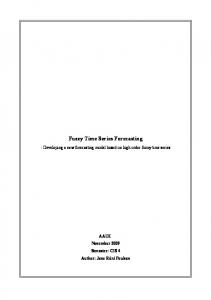
Figure 2 shows the predictions of a forty-state HFHMM that was trained for seventy iterations of the forward-backward algorithm, as described in [2]. The forecast diverges rapidly, becoming inaccurate in fewer than ten steps, and the probability density of the prediction “leaks” away from the range of the time series. Figure 3 shows the predictions of a simulation using a twenty state “seed” MSMM, that has not been iteratively optimized. It accurately predicts the behavior of the time series for about 35 steps, then it mistakenly predicts a transition to the upper half of the attractor and continues to predict values within the attractor until the end of the simulation at time T + 100. The divergence near the end is an artifact of the simulation algorithm, since paths that are just beginning to “leak” at the end of the simulation are not discovered and discarded. We have developed a very crude hill-climbing method that can somewhat improve seed MSMMs. Applying the method to the model that produced Fig. 3 yields forecasts that seem no different by eye from those of the seed model, although there is somewhat less leakage and the medium-range estimates are more accurate. We are currently investigating more efficient methods of optimization. As figure 2 demonstrates, when a HFHMM is fit to chaotic dynamics probability will leak away to exponentially larger values of y as the number of time steps is increased. Considering the Lyapunov exponents helps explain this defect. A discrete state sequence sτ1 specifies a sequence of linear maps, i.e., derivative information. For typical long sequences, the magnitudes of the eigenvalues of the products of these maps will grow at exponential rates given by the Lyapunov exponents. For chaotic systems, at least one Lyapunov exponent is positive, and the composed maps are linearly, and hence globally, unstable. The problem is that the model is affine (linear plus constant) in ¯ and a the sense that for a given state sequence, there is a constant vector x τ τ constant sequence y¯1 such that for any sequence of observations y1 , history
9
x, and λ ∈ R Pθ (y1τ | sτ1 , x(1) = x) = P (λy1τ + (1 − λ)¯ y1τ | sτ1 , x(1) = λx + (1 − λ)¯ x). Thus a HFHMM fit to a chaotic process will be unstable. A MSMM includes an output model that has exactly the same property: given a transition s(t) → s(t + 1) (rather than a state, as for a HFHMM), the
output y(t) is modeled as an affine linear function of the output history. We introduced these history dependent transition probabilities in an attempt to make the probabilities of the divergent sequences small. We do not yet have working programs that optimize such models, and the seed models do not quench the divergence, but the model parameters permit the computation of P (x(t)|s(t), s(t + 1)), and we have used this information in an ad hoc fashion to quench divergence; we simply delete all paths for which P (x(t)|s(t), s(t + 1)) is zero to machine precision. The surviving paths are necessarily close to the training data.
Summary MSMMs are a powerful way to model non-linear processes. For some applications[2] a suboptimal version of the forward-backward algorithm gives good results. For the Double Scroll data, it is inappropriate, and we have foregone optimization altogether. The Double Scroll system has been useful for illuminating both the strengths and weaknesses of our techniques. We are working on an optimal version of the forward backward algorithm for MSMMs, and we hope it will produce models that forbid divergent behavior.
References [1] L. O. Chua, M. Komuro, and T. Matsumoto. The Double Scroll family. IEEE Trans. Circuits Syst., CAS33:1072–1118, Nov. 1986. 10
[2] A.M. Fraser and A. Dimitriadis. Hidden Markov models with mixed states. In A. Weigend and N. Gershenfeld, editors, Predicting the Future and Understanding the Past: a Comparison of Approaches. AddisonWesley, 1993. [3] A. M. Fraser and Q. Cai. Detecting chaotic signals with nonlinear models. In Proc. IEEE SSAP workshop, Oct. 7-9, 1992 Victoria BC., 1992. [4] L.E. Baum, T. Petrie, G. Soules, and N. Weiss. A maximization technique occurring in the statistical analysis of probabilistic functions of Markov chains. The Annals of Mathematical Statistics, 41(1):164–171, 1970. [5] A.B. Poritz. Hidden Markov models: A guided tour. In Proc. IEEE Intl. Conf. on Acoust. Speech and Signal Proc., 1988. [6] J.D. Ferguson. Hidden Markov analysis: An introduction. In Proc. of the Symposium on the Applications of Hidden Markov Models to Text and Speech, pages 8–15, Princeton, 1980. IDA-CRD. [7] W. H. Press, B. P. Flannery, S. A. Teukolsky, and W. T. Veterling. Numerical Recipes in C. Cambridge University Press, Cambridge, 1988. [8] A. Gersho and R. M. Gray. Vector Quantization and Signal Compression. Kluwer, Norwell MA, 1992.
11
Alexis Dimitriadis received his Bachelor’s degree in Biology from Reed College, Portland, Oregon in 1986, and the Master’s of Arts in Mathematics from Portland State University in 1992. In 1988 he worked on statistical analysis of on-line DNA databases at the University of Crete, Greece. From 1990 to 1992 he was a Research Assistant in the Systems Science Ph.D. Program at Portland State University, where he worked on the modeling of real valued time series. He is currently studying Linguistics at the University of Pennsylvania. Andrew M. Fraser received the Bachelor’s degree in Physics from Princeton University in 1977 and the Ph.D. degree in Physics from the University of Texas at Austin in 1988. From 1977 to 1981, as a Design Engineer at Fairchild Semiconductor in Mountain View, CA, he worked on bipolar PROMs and implemented a fused-emitter PROM technology. As a graduate student at the University of Texas, he worked on the information theoretic characterization of chaotic time series. Dr. Fraser has been at at Portland State University since 1989, where he is currently an Assistant Professor in both the Systems Science Ph.D. Program and the Department of Electrical Engineering. He is currently working on models for chaotic time series.
12
(a)
0.40
0.24
y2
0.08
-0.08
-0.24
-0.40 -3.0
-1.8
-0.6
0.6
1.8
3.0
240
320
400
y1
3.0
(b)
1.8
y(t)
0.6
-0.6
-1.8
-3.0 0
80
160
t
Figure 1: A chaotic attractor. A phase portrait of the Double Scroll system appears in (a), and in (b) this vector trajectory has been projected down to a scalar time series.
13
(a)
6.0
4.0
y(T+t)
2.0
0.0
-2.0
-4.0
-6.0 0
2
4
6
8
10
12
14
16
18
20
t
(b)
6 4 2
P(y(t))
0 -2
0.5 0 0
-4 5
10
15
20
25
30
35
40
y
-6
t
Figure 2: Probability forecast computed via Monte Carlo simulation using a HFHMM with fourth-order autoregressive outputs and 40 hidden states. The model was fit to a 40,000 point time series in 70 iterations of the forwardbackward algorithm starting with a seed model that was based on vector 40,020 appears as a smooth quantization. In (a) the actual continuation data y40,001 horizontal curve, and at each time step t a forecast density Py(t) is superposed on the time series plot. The density14plots are discontinued over regions in which the forecast density is zero. Probability beyond bins at ±4.4 are accumulated and plotted in the end bins. At later times, as the forecast density function spreads out, these end bins accumulate most of the probability. (b) is a perspective plot of the same data.
(a)
6.0
4.0
y(T+t)
2.0
0.0
-2.0
-4.0
-6.0 0
5
10
15
20
25
30
35
40
45
50
t
(b)
6 4 2
P(y(t))
0 1 -2 0 0
-4 20
40
60
80
100
y
-6
t
Figure 3: Probability forecast computed via Monte Carlo simulation using a MSMM. This model is fourth-order autoregressive and has 20 discrete (hidden) states. It was estimated directly from vector quantization of the training data. As in fig. 2, two representations of the forecast density functions appear in (a) and (b). 15