Modeling for (physical) biologists: an introduction to the rule-based

Home

Search

Collections

Journals

About

Contact us

My IOPscience

Modeling for (physical) biologists: an introduction to the rule-based approach

This content has been downloaded from IOPscience. Please scroll down to see the full text. 2015 Phys. Biol. 12 045007 (http://iopscience.iop.org/1478-3975/12/4/045007) View the table of contents for this issue, or go to the journal homepage for more

Download details: IP Address: 129.59.115.15 This content was downloaded on 17/07/2015 at 07:06

Please note that terms and conditions apply.

Phys. Biol. 12 (2015) 045007

doi:10.1088/1478-3975/12/4/045007

PAPER

RECEIVED

20 November 2014

Modeling for (physical) biologists: an introduction to the rule-based approach

REVISED

25 February 2015 ACCEPTED FOR PUBLICATION

Lily A Chylek1,2, Leonard A Harris3, James R Faeder4 and William S Hlavacek2,5

9 March 2015

1

PUBLISHED

2

15 July 2015 3 4 5

Department of Chemistry and Chemical Biology, Cornell University, Ithaca, NY 14853, USA Theoretical Biology and Biophysics Group, Theoretical Division and Center for Nonlinear Studies, Los Alamos National Laboratory, Los Alamos, NM 87545, USA Department of Cancer Biology, Vanderbilt University School of Medicine, Nashville, TN 37212, USA Department of Computational and Systems Biology, University of Pittsburgh School of Medicine, Pittsburgh, PA 15260, USA New Mexico Consortium, Los Alamos, NM 87544, USA

E-mail: [email protected] and [email protected] Keywords: rule-based modeling, systems biology, cell signaling Supplementary material for this article is available online

Abstract Models that capture the chemical kinetics of cellular regulatory networks can be specified in terms of rules for biomolecular interactions. A rule defines a generalized reaction, meaning a reaction that permits multiple reactants, each capable of participating in a characteristic transformation and each possessing certain, specified properties, which may be local, such as the state of a particular site or domain of a protein. In other words, a rule defines a transformation and the properties that reactants must possess to participate in the transformation. A rule also provides a rate law. A rule-based approach to modeling enables consideration of mechanistic details at the level of functional sites of biomolecules and provides a facile and visual means for constructing computational models, which can be analyzed to study how system-level behaviors emerge from component interactions.

Introduction A model is a representation or imitation of a system. A model is especially useful when the system of interest is both complex and difficult to probe experimentally. Models have long been used to study biological systems, which are among the most complex systems studied in science and engineering. Models take many different forms. Two types of models that are familiar to biologists are (1) a living system amenable to experimental study (e.g., an animal in which characteristic features of a human disease are recapitulated, a mammalian cell line, or a model organism, such as Escherichia coli, Saccharomyces cerevisiae or Caenorhabditis elegans) and (2) a diagram, which is often used to graphically summarize one’s understanding of how a system operates. Aspects of these two types of models, living systems and diagrams, are combined in mathematical/ computational models. (We will hereafter refer primarily to computational models, because the vast majority of mathematical models are now analyzed with the aid of computers, and models formulated as © 2015 IOP Publishing Ltd

computer programs, meaning computational models, are becoming more common and almost always have an underlying mathematical basis.) Like a diagram, a computational model is based on what a modeler knows or hypothesizes about a system. A difference is the greater precision of a computational model. Whereas a diagram tends to be ambiguous and qualitative, a computational model requires a modeler to make concrete, quantitative statements about how a system is believed to behave. The precision and rigor required to build a computational model can help to identify gaps in knowledge and understanding. When such gaps are encountered, a modeler is required to generate hypotheses that fill the gaps. Knowledge and hypotheses are formalized and used to create a set of equations and/or a computer program, which can be used, for example, to simulate how the state of a system evolves over time in response to a stimulus or perturbation. In this way, a computational model shares an important feature of a living model system: both a computational model and a living model enable biological phenomena to be studied in a controlled manner, in a setting that allows questions about system

Phys. Biol. 12 (2015) 045007

L A Chylek et al

behavior and mechanisms to be answered with relative ease. Both types of models suffer from the pitfall that the insights obtained may depend in an unknown way on the degree to which the model at hand represents the true object of study, the biological/physiological system of interest. Nevertheless, models are essential for progress in biological research, because many questions simply cannot be studied without them. Biologists routinely use diagrams to reason about biological systems, especially cellular regulatory networks. In the context of discussions about cell signaling systems, these diagrams are sometimes called pathway maps, or simply maps. Pathway maps, which are commonly drawn ad hoc, despite attempts to establish standardized conventions [1], can be viewed as a type of conceptual model. A map can be used to summarize and convey one’s understanding of how a system works or to provide a broad overview of what is known about a system. A limitation of a map is that its interpretation ultimately relies on the intuition of its reader, which is a serious weakness given the complexity of cellular regulatory networks. The complexity of cellular networks arises from several sources. One is the ubiquitous presence of feedback and feedforward loops, which can generate exotic nonlinear behaviors, such as hysteresis and oscillations [2, 3]. Another complicating feature is the tendency of the biomolecules that comprise cellular regulatory networks to interact with multiple binding partners [4, 5]. This molecular promiscuity, or polyspecificity, can generate crosstalk, meaning influences between networks with distinct functions. Another complication is that biomolecular interactions and their consequences are sensitive to quantitative factors, including the copy numbers of binding partners, binding cooperativity, and binding affinities and lifetimes [6, 7]. In addition to these quantitative properties of biomolecular interactions, which can be viewed as intrinsic properties, interactions are also likely to be affected by extrinsic properties, such as compartmentalization [8] and binding competition within a compartment [9], which is a function of network connectivity. The features mentioned above can either alone or in combination give rise to non-intuitive system behaviors. These complicating features limit our ability to understand and manipulate cellular regulatory networks, and they beckon us to consider models more sophisticated and powerful than diagrams, such as computational models. Computational models go beyond diagrams, because the logical consequences of the information used to formulate a model can usually be elucidated through computer-aided calculations, or simulations. The information that serves as the basis for a model may include a synthesis of multiple mechanistic insights, an integration of different types of quantitative data (e.g., measurements of protein copy numbers and dissociation constants), and plausible assumptions, which are often necessary to fill knowledge gaps 2

as noted earlier. The analysis of a computational model can identify a potential system behavior that one would not have expected and suggest experiments to test the non-obvious (i.e., interesting) predictions of the model. Validation of such predictions increases one’s confidence in the model. Falsified predictions can also be useful if they lead to revisions that increase a model’s reliability and generality. Modeling is not a monolithic practice. Different techniques are used to address different problems. Even the same problems are commonly attacked using a variety of techniques. Some models are formulated to study specific systems, whereas others are formulated to study phenomena found in many systems. The physical and chemical principles captured in models vary, and models incorporate biological knowledge at differing resolutions, from abstract and phenomenological to detailed and mechanistic [10]. Some approaches, such as logical modeling [11], are unconnected or only loosely coupled to physicochemical principles. This diversity reflects not only a need for different approaches to address different questions but also a lack of consensus about best practices. Arguably, the field of computational systems biology is at a stage where many different modeling approaches are being tried partly because traditional modeling approaches, meaning those long used, mostly in non-biological fields, have shortcomings when applied to biological systems. Models based on ordinary differential equations (ODEs) are arguably the most popular type of physicochemical model employed in biology [12]; these models represent a traditional modeling approach. ODEs have been used to model (bio)chemical systems since before the existence of molecules was widely accepted [13, 14]. Although ODE models are undoubtedly useful, the ODE modeling approach when applied to cellular regulatory networks entails complicating requirements that call for new ideas about how to model [15–17]. Namely, this approach requires one to enumerate the potentially populated chemical species in a system. Because biomolecules can usually be found in numerous states and complexes, it is desirable to avoid this requirement. Rule-based modeling allows one to avoid enumerating the potentially populated chemical species in a system; it is an approach tailored for modeling a biomolecular interaction network, or indeed, any system where structured objects interact via component parts in a modular way. Here, we provide a brief introduction to rule-based modeling in systems biology, which is characterized by the use of local rules to represent biomolecular interactions [18–24]. In biology, rulebased modeling has most often been used to study cell signaling systems, but this modeling paradigm is more broadly applicable [23, 25–27]. Indeed, rule-based modeling has antecedents in physics, chemistry, and computer science [22, 28–32]. Rules formalize mechanistic understanding of biomolecular

Phys. Biol. 12 (2015) 045007

L A Chylek et al

interactions according to conventions that allow a set of rules to serve as an executable model, meaning a model that can be used to obtain simulations of the behavior of the system represented by the model. Simulations may leverage different algorithms to capture system behavior at varying levels of abstraction of the underlying physiochemical laws. For example, simulations are possible that do and do not account for fluctuations in copy numbers, depending on how the simulation algorithm relates to the chemical master equation [33]. Once a rule-based model is specified, it is relatively easy to perform multiple types of simulations, which facilitates analysis. For example, one can readily switch between stochastic and deterministic simulation methods [34]. A rule-based approach to model specification is most justified when one is concerned with biomolecular interactions that depend on and impact site-specific details, or biomolecular site dynamics [23], and moreover the interactions of interest are modular, meaning somewhat independent of each other. Many rule-based models reported in the literature are simulated using an ODE solver operating on rulederived ODEs, and so can be viewed as equivalent to ODE models that produce the same simulation results. However, rule-based models are specified in terms of rules instead of equations. The different approaches used to specify ODE and rule-based models are not superficial; the differences in the way these models are written (i.e., specified) encourage and usually entail different modeling assumptions. This review, mainly through discussion of examples of rules and simple but complete executable models, is meant to help biologists, including those who do not specialize in modeling, create models for the systems they study. Models can serve as valuable reasoning aids, and with rule-based modeling, more widespread use of models is foreseeable. This review may also be helpful for experienced modelers new to rule-based modeling, or even practitioners of the approach, because the example models illustrate a variety of rule-based modeling capabilities and may therefore serve a valuable reference purpose. We will focus on one particular approach that can be used to specify and analyze rule-based models, the approach enabled by the BioNetGen language (BNGL) and BNGL-compatible software tools, such as BioNetGen [34–36]. Our focus will also be on models appropriate for well-mixed reaction compartments, because such models are generally easier to specify and analyze. With such models, there is no need to specify reaction compartment geometry or boundary conditions, for example. Later, we will mention other model-specification approaches and software tools (many with capabilities beyond what is offered by the BNGL framework) and point to sources of information about these methods. A tight focus is necessary to provide a practical introduction to rule-based modeling and concrete examples. After learning the principles 3

taught here, we encourage readers to explore other approaches.

What makes models useful? Models have the potential to aid biologists in several ways. First, a model can be used as a roadmap for experimental design. Experiments are used to test hypotheses, and the more complex a hypothesis, the more complicated and numerous the necessary experimental tests are likely to be. Models can potentially be used to carefully design experimental tests that would be optimal for supporting or disproving a hypothesis [37–39]. Second, models can also be used to reconcile surprising or conflicting data. In some cases, seemingly contradictory results may actually be compatible when quantitative details are taken into account [40]. Third, models can be used to consolidate knowledge about a system [41, 42]. Analogous to assembly of a jigsaw puzzle, models can be used to piece together available information to form a more complete picture of how a system works. Furthermore, by comparing model-based simulations to experimental data, discrepancies between understanding and reality can be identified, which may point to areas where additional pieces of information need to be discovered through further experiments. What constitutes a useful model? The answer to this question depends partly, or even largely, on current modeling capabilities. For example, models that require computer-aided operations to obtain predictions of system behavior (e.g., generation of random numbers as in Monte Carlo methods [43]) only became useful after technological advances made analyses of such models practical. It has recently been argued that those pursuing useful models in biology should adhere to the following guidelines [44]: (1) ‘ask a question’, (2) ‘keep it simple’, and (3) ‘if the model cannot be falsified, it is not telling you anything’. The latter guideline represents valuable advice, because if a model cannot be falsified, it lies outside the realm of science. However, this guideline should perhaps be augmented with an admonition to seek models that make not only testable predictions but also unexpected predictions. The first two guidelines also represent valuable advice, although their interpretation should not be static. These guidelines must be tempered with an awareness of what current modeling methodology allows. For example, although ‘asking a question’ is necessary as a starting point, it does not mean that a model need be designed/used for only a single purpose to the exclusion of model reuse [45], which can be valuable and time saving. Similarly, ‘keeping it simple’ is partly defined by the tools and data available to a modeler; what appears complex using one modeling approach may actually be simple using another. For example, the development of rulebased modeling approaches, as we will see below, has

Phys. Biol. 12 (2015) 045007

L A Chylek et al

made it relatively easy to specify models that would be cumbersome if not impossible to specify as ODEs. Simplicity is viewed as a virtue, perhaps especially so in mathematical pursuits, such as modeling. In his famous lecture on mathematical problems, Hilbert stated [46], ‘what is clear and easily comprehended attracts, the complicated repels us’. A view among some, if not most, modelers is that many biochemical details elucidated by biologists are too complicated to contemplate including in models. Accordingly, many known biochemical details are omitted in models. Simple, abstract models, which may focus, for example, on capturing certain limited influences among molecular entities and processes, have certainly been useful [47, 48], and are likely to continue to be useful for a long time. However, there are many important questions that can now be feasibly addressed that depend on consideration of biochemical details to an extent beyond what is usually considered by modelers. Easing the consideration of mechanistic biochemical details in models for cellular regulatory systems was one of the driving motivations for the development of the rule-based modeling approach in systems biology [18]. With this approach, there is a new definition of ‘simple’. We should heed the saying attributed to Einstein [49], ‘everything should be as simple as possible, but not simpler’. The ability to capture mechanistic details in a rulebased model has opened new frontiers, such as the development of ‘standard models’, which do not currently exist in most if not all of biology. Standard models in other fields, such as the Standard Model of particle physics [50], drive the activities of whole communities and tend to be detailed, because they consolidate knowledge and are useful in large part because they identify the outstanding gaps in understanding. Would standard models benefit biologists? An affirmative answer is suggested by the fact that there are many intricate cellular regulatory systems that have attracted enduring interest, such as the epidermal growth factor receptor (EGFR) signaling network [51, 52], which has been studied for decades for diverse reasons. Efforts to model EGFR signaling have been hailed as paradigmatic of systems biology [53]. A comprehensive, extensively tested, and largely validated model for the EGFR signaling network or any other well-studied system, meaning a standard model, would aid modelers by providing a trusted reusable starting point for asking not one but many questions.

Uses and advantages of rule-based modeling Rules describe the interactions and processes in a system. Various established conventions exist for writing rules, such as BNGL [34], but in each of these, a modeler specifies (1) the properties required of reactants, (2) the outcome of a reaction, or, 4

equivalently, the transformation that is applied to reactants to obtain products, and (3) the rate law that governs all reactions implied by the rule. A rule is minimal if it does not depend on any properties of the reactants other than those of the components that are modified by the reaction. For example, a minimal rule for association might only require that each of the two sites participating in formation of a non-covalent bond be free. The set of sites or molecular components modified by a rule is called the reaction center. Any additional requirements on the reactants are considered contextual. When the interactions in a system are known to be modular, the rules describing the system will incorporate relatively little information about molecular context and the contextual requirements that are expressed in rules will be local, such as a requirement that a site neighboring a reaction center be bound or in a particular modification state. Rules for the interactions in a cellular regulatory network provide a high-level and relatively easy-to-obtain representation of the network. As we will discuss later, the rules of a model can often be translated automatically into equations, which can then be analyzed using conventional numerical methods. In cases where translation of rules into equations is not possible, the rules of a model can be used as event generators in a discrete-event (stochastic) simulation algorithm. Because rules can include information about specific biomolecular sites, such as a constraint limiting an interaction between two proteins to cases where a particular tyrosine residue in one of the proteins is phosphorylated, rule-based modeling is ideal for representing biomolecular site dynamics, the changes in states occurring at the functional sites of biomolecules [23]. For proteins, these sites include conserved domains [54], such as Src homology 2 (SH2) and SH3 domains [55], as well as catalytic domains; short linear motifs [56]; and sites of post-translational modifications [57], such as an amino acid residue modified through covalent enzyme-catalyzed addition of a chemical group (e.g., a phosphoryl group) or a peptide bond that can be cleaved by a protease. The concept of a rule, which provides an abstract representation of an interaction (or process), should become clearer as we discuss examples. Rules can be specified using many different conventions and means [35, 58–70]. Here, as indicated earlier, we will focus on use of the BNGL [34] for specifying rules. Many of the available rule-based models, which are essentially collections of rules, have been formulated using this language [71] or can be readily recast in this language. Much of what is said here about BNGL and BNGL-compliant software also applies to other model-specification languages and the software compatible with these languages, which will be briefly discussed later. Several thorough but informal descriptions of BNGL are available [34, 72, 73]. A formal description is also available [74]. BNGL allows for the specification

Phys. Biol. 12 (2015) 045007

L A Chylek et al

of complete, executable models, which again can be viewed as collections of rules, as well as parameter values and other ancillary information (e.g., initial conditions). BNGL also allows for the specification of actions, which include simulation protocols, and simulation outputs. BNGL is a machine-readable (i.e., textbased) language designed for modeling cellular regulatory systems (especially cell signaling systems), which is akin to a domain-specific programming language. It is compatible with a number of general-purpose software tools, including BioNetGen [34, 35], RuleBuilder [75], RuleBender [76, 77], MOSBIE [78], DYNSTOC [79], RuleMonkey [80], and NFsim [81]. Once specified, a BNGL-encoded model can be processed to perform different operations, including model visualization; translation of a BNGL-encoded model specification into different formats, such as an equivalent systems biology markup language (SBML) encoding [12] or a MATLAB M-file or MEX-file [82]; and simulation [34]. A variety of simulation methods (and simulators) are available [23], as we will discuss later. It is important to understand how rule-based models differ from traditionally formulated models to appreciate when a rule-based approach is warranted and most likely to be helpful. As indicated earlier, a key distinction between a rule-based model and a traditional equationbased model is the way that it is specified, but there tend to be important differences beyond the means of specification. We note that equation-based models that are comparable to rule-based models may take the form of ODEs for systems with well-mixed chemical kinetics or the form of partial differential equations (PDEs) for systems in which reaction and diffusion are coupled. Although one could in principle use either rules or equations to specify essentially the same model for a system of interest, the different model-specification approaches tend to engender different modeling assumptions. Indeed, when one compares models in the literature, such as the ODE-based models of Kholodenko et al [83] and Chen et al [84] for ErbB receptor signaling and the rule-based models of comparable scope of Blinov et al [85] and Creamer et al [86], one sees that the different types of models are based on very different assumptions. Equation-based models are based on assumptions about which chemical species are populated and therefore tracked. Thus, the size of a model corresponds to the number of chemical species taken to be populated in a system. Rule-based models, in contrast, are based on assumptions about the modularity of interactions, which affect the forms taken by rules. The size of a model corresponds to the number of interactions of interest. These differences arise from the distinct approaches to model specification, which have different requirements. To specify an ODE or PDE model, for example, one must enumerate the chemical species that are potentially populated and write an equation for each. Thus, in modeling a cell signaling system with ODEs or PDEs, a modeler is obligated to specify which protein states and signaling complexes are populated. 5

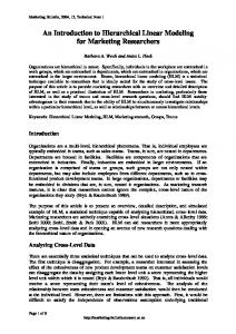
Unfortunately, there is usually no empirical data available to guide a modeler in deciding which chemical species and reactions are important, and a comprehensive enumeration of all possibly populated chemical species is often impracticable. When site dynamics are considered there may be more chemical species that could potentially be populated than there are molecules in a cell. This barrier to model specification has been called combinatorial complexity [15, 16]. We note that lack of information about which chemical species are populated in a system is an issue of concern even if one takes a rule-based modeling approach (which eliminates the requirement to enumerate chemical species), because this information, if available, would impose useful constraints on the rules of model. However, the rules and parameters of a rule-based model implicitly identify important species and reactions, which can be revealed through simulation [87]. Thus, a rule-based modeling approach does not eliminate the problem of absence of knowledge about the important chemical species and reactions in a system but it does provide a tool for discovering this information starting from the known biomolecular interactions of the system. An example of combinatorial complexity is provided in figure 1(A), which illustrates the reaction network that arises in a model for a protein with two phosphorylation sites that can bind other proteins when phosphorylated. This model implies a reaction network with 9 distinct chemical species and 12 possible reactions, but it can be encoded with a set of four rules under the assumption that phosphorylation or binding at one site does not affect the rate of reactions taking place at the other site. The use of rules (figure 1(B)) circumvents the requirement to identify the possible chemical species and reactions in advance and greatly reduces the size of the model specification in this case (from 12 reactions to 4 rules). Each rule specifies the necessary and sufficient conditions for occurrence of the interaction represented by the rule. In our example, each rule only specifies the state of the site being modified by phosphorylation or binding, but not that of the other site. Each rule generates a reaction for each allowable set of reactant species it encounters, and furthermore, each reaction generated by a rule is parameterized by the same rate constant. The latter represents a coarse graining of the chemical kinetics, because in principle, each species may be associated with a unique reactivity, as suggested by figure 1(A). The effect of this modularity assumption is shown in figure 1(C), where each of the three reactions generated by each rule is governed by the same rate constant. This rule-based version of the model is thus not quite as general as the full reaction scheme. Although rules tend to involve assumptions of modularity, rules can be made as precise as necessary to represent knowledge or hypotheses about the underlying biochemistry. It would be possible, for example, to use rules to fully specify the reaction network shown in figure 1(A) using a set of 12 rules

Phys. Biol. 12 (2015) 045007

L A Chylek et al

Figure 1. Reaction network-based and rule-based representations of a simple biochemical system. (a) Reaction network for a protein (rounded box) that can be phosphorylated and modified at two sites. The unmodified forms and phosphorylated forms of each site are represented by an open circle and filled circle, respectively. Binding of another protein to a phosphorylated site is indicated by addition of an edge. Because of combinatorial complexity, there are a total of nine possible chemical species (labeled s1–s9) corresponding to distinct states of phosphorylation and binding, with a total of 12 possible (bio)chemical reactions (labeled r1–r12) connecting these states. Although such transformations are reversible in general, we have made the reactions unidirectional here for simplicity. (b) Rules with modularity assumptions that represent the network with simplifying rate assumptions. Each of the four rules describes a transformation, either phosphorylation or binding, that occurs at one of the two sites. Because each rule refers to only one site, the state of the other site affects neither the applicability of the rule nor the rate of the reactions that are generated. (c) Reaction network generated by the modular rules in (b). Labels on the reaction arrows indicate the rate constants governing each reaction. Each rule generates three reactions with identical rate constants as indicated. Although the number of species and reactions is the same as the network shown in (a), the number of parameters governing the rate equations in the model has been reduced from 12 to 4 by neglecting possible cooperative interactions between the sites. (d) Simplified reaction network models with assumptions to limit combinatorial complexity. Two types of common implicit assumptions are illustrated: sequential modification, where the modifications of the sites are assumed to occur in a particular order, and competitive binding, where only one binding partner is allowed to bind at a time. These assumptions limit both the reaction network size and the number of parameters. All but one of the reactions depicted has a corresponding transformation in the rule-based version of the model (c), as indicated by the index of the rate constants. A prime is used to denote approximate correspondence, because the underlying assumptions of the models differ. The competitive binding model also includes a lumped reaction in which both sites are assumed to be phosphorylated to enable binding of one or the other of the protein’s binding partners.

having more contextual constraints than the four rules discussed above, making each of these rules as specific in regards to reactants as the 12 distinct reactions. Thus, these rules would be equivalent to or essentially the same as the reactions shown in figure 1(A). Such a specification would not be more concise than a traditional one, but it would have the advantage that the precise structural (i.e., site-specific) requirements for each reaction would be recorded in the rules. Rule-based modeling can be viewed as a generalization of traditional approaches to modeling 6

biochemical kinetics that lifts the burden of needing to make an explicit listing of the chemical species and reactions that are important in a system. The burden of enumerating species and reactions often leads to ad hoc assumptions to limit the number of species and reactions included in a model. Two such assumptions are illustrated in figure 1(D). Both reaction schemes include the same types of reactions (binding and phosphorylation) used in the full and rule-based versions, but the majority of species and reactions are eliminated. Although assumptions of sequential

Phys. Biol. 12 (2015) 045007

L A Chylek et al

modification or competitive binding may be justified in some cases, expedience is often the (unstated) rationale. Because traditional modeling approaches also lack standard nomenclature for tracking bonds or post-translational modifications, the composition of species can be ambiguous and the nature of assumptions made in constructing a model difficult to assess. Although cell signaling has been studied for decades, we have limited knowledge about how modifications and binding at different sites of a protein are coupled (e.g., [20, 24, 88]). We argue that rules expressing a high degree of modularity represent a more natural starting point for model development than making assumptions for the sake of limiting network size. At the same time we caution that assumptions of modularity may not always be valid, as exemplified by the model of Ullah et al [89] for the behavior of a ligand-gated ion channel, the inositol 1, 4, 5-trisphosphate receptor. This model includes only a fraction of the possible states of the receptor, those identified as being critical for reproducing an impressive collection of data. Although the model is inconsistent with ligand binding sites in the receptor behaving independently, or modularly, the states included in the model are highly idiosyncratic, meaning that the importance of these particular states is not at all apparent. Thus, this model is representative of models having structures that can only be found through inference from data. Models, especially at early stages of investigation, are usually taken to have less labyrinthine structures, regardless of modeling approach. Successive refinement of modular rules represents one principled approach that may prove useful in the future for the inference of such complex cooperative interactions from data.

Examples of rules for interactions in a cell signaling system To make the concept of rules more concrete, let us introduce and then discuss three sets of BNGLencoded rules, which describe various processes involved in IgE receptor (FcεRI) signaling (figure 2). (As we discuss these rules, we will also discuss the underlying biological details, hopefully in an intelligible manner for readers unfamiliar with FcεRI signaling.) These rules are drawn from a larger set of such rules

[41], discussed below, and do not by themselves form a coherent model of the system. Before discussing the example rules and presenting them in BNGL format, it should be noted that rules generally encode molecular mechanisms, which may seem arcane and which can make the writing or interpretation of a rule somewhat challenging. Of course, the ability to naturally capture (i.e., formalize) molecular mechanisms of biomolecular interactions is an advantage of rules, but because of the intimate link between the form of a rule and the underlying biological details, the presentation of rules below is necessarily entwined with a discussion of molecular mechanisms (i.e., site-specific details of biomolecular interactions) involved in FcεRI signaling. If these details obscure our introduction of rules (which we hope is not the case), we encourage the reader to return to this section after examining the complete models discussed later; these models consist of rules that can be interpreted more easily without background knowledge about a particular biological system. FcεRI is a multichain antigen recognition receptor that is expressed, for example, on mast cells [90]. The antigen specificity of a given FcεRI receptor is determined by the IgE antibody with which the receptor is associated. IgE-FcεRI complexes are long lived relative to the time scale of the signaling events initiated by the interactions of IgE-FcεRI complexes with a multivalent antigen. Signaling may be initiated in the laboratory by crosslinking of FcεRI through use of various reagents, such as bivalent haptens, multivalent haptenated proteins (or other carrier molecules), chemically crosslinked oligomers of IgE, anti-IgE antibodies, and anti-FcεRI antibodies [91]. Here, we will discuss rules for the following signaling processes, which can all be considered early steps in FcεRI signaling (figure 2(A)): (1) binding and crosslinking of receptors by a bivalent anti-FcεRI IgG antibody (figure 2(B)); (2) recruitment of a protein tyrosine kinase, Lyn, to a docking site at Y218 in the β chain of an activated receptor (UniProt [92] numbering for the rodent protein Ms4a2), which depends on phosphorylation of Y218 (figure 2(C)); and (3) phosphorylation of a membrane-localized substrate (Y175) in Lat by a second receptor-associated protein tyrosine kinase, Syk (figure 2(D)). Rules for these processes can be written in BNGL as follows:

Lig (r,r) + Rec (l)−> Lig (r,r ! l). Rec (l ! 1) kp1

(1a)

Lig (r ! + ,r) + Rec (l) −> Lig (r ! + ,r ! 1). Rec (l ! 1) kp2

(1b)

Lig (r ! 1). Rec (l ! 1) −>Lig (r) + Rec (l) koff

(1c)

Lyn (SH2) + Rec (b_Y218 ∼ P) < − > Lyn (SH2 ! 1). Rec (b_Y218 ∼ P ! 1) kp1,kmL

(2)

Syk (tSH2 ! + ,kin) + Lat (Y175 ∼ 0)−> Syk (tSH2 ! + ,kin ! 1). Lat (Y175 ∼ 0 !1) kf

(3a)

Syk (kin ! 1). Lat (Y175 ∼ 0 ! 1)−> Syk (kin) + Lat (Y175 ∼ 0) kr

(3b)

Syk (kin ! 1). Lat (Y175 ∼ 0 ! 1)−> Syk (kin) + Lat (Y175 ∼ P) kcat

(3c)

7

Phys. Biol. 12 (2015) 045007

L A Chylek et al

These rules, which represent direct binding and catalytic interactions, are visualized in figure 3 in accordance with the conventions of Faeder et al [93]. Note that bonds between molecular components are indicated by sharing of bond indices, which are prefixed by the ‘!’ symbol. The notation ‘!+’ indicates a bond without indicating the binding partner. Similarly, internal states of molecular components are prefixed by the ‘∼’ symbol. The conventions of BNGLencoded rules are discussed further below. The rule of equation (1a) represents capture of a free ligand by a free receptor site, meaning capture of free anti-FcεRI IgG antibody by the epitope in FcεRIα recognized by the antibody. The rule of equation (1b) represents crosslinking of two receptors by a receptortethered ligand. The rule of equation (1c) represents dissociation of a ligand–receptor (non-covalent) bond. Note that in the graphical depictions of these interactions, which are shown in figures 2(B) and 3(A), (B), the two binding rules are depicted as reversible, whereas in equation (1c) we have combined the two types of dissociation events captured in the reversible rules into a single dissociation rule. The rule of equation (2) represents reversible recruitment of the Src-family protein tyrosine kinase Lyn to a phosphotyrosine docking site in the receptor via Lyn’s SH2 domain. The docking site is located at Y218 in the receptor’s β chain, which is part of an immunoreceptor tyrosine-based activation motif (ITAM). The rules of equations (3a) through (3c) represent Sykmediated phosphorylation of a substrate in the membrane adaptor protein Lat (Y175, UniProt numbering for the rodent protein) via a Michaelis–Menten mechanism [94, 95]. The rule of equation (3a) indicates that a component in Syk, which is named tSH2 to suggest ‘tandem SH2 domains,’ is bound, which is indicated by the notation ‘!+.’ (The tandem SH2 domains in Syk interact with a pair of ITAM phosphotyrosines in each of the receptor’s γ chains.) Thus, the rule of equation (3c) represents an activity of Syk that is restricted to receptor-associated forms of this protein tyrosine kinase, because binding of the kinase domain of Syk, denoted kin, to its substrate, Y175 in Lat, depends on Syk association with the receptor, as indicated by the rule of equation (3a). As can be seen from the example rules presented above, formal elements of a rule are often in one-toone correspondence with material entities. For example, Lyn in the rule of equation (2) refers to Lyn and SH2 refers to the SH2 domain of Lyn. Each of our example rules ends with a listing of either one or two names of parameters. These ruleassociated parameters are, by convention, taken to be rate constants in mass-action (elementary) rate laws. (Other types of rate laws can also be associated with rules, but when only a parameter name is given, a mass-action rate law is implied by convention.) The numerical values (and the units) of the rate constants associated with rules are 8

usually defined separately from the rules within a model-specification file. There is at least one rate law associated with each rule. Reversible rules, such as the rule of equation (2), may be associated with two rate laws, one for the forward transformation defined by the rule and one for the reverse transformation defined by the rule. The rule of equation (2) is associated with two rate constants and has two directions. It can be viewed as a generalized reversible reaction, or a reaction generator that defines forward and reverse transformations arising from a reversible interaction between two molecules named Lyn and Rec. The rule indicates that the interaction between Lyn and the receptor is mediated by molecular components named SH2 (a constituent of Lyn) and b_Y218 (a constituent of FcεRI’s β-chain ITAM). The nomenclature of rules is similar to that of standard chemical reactions; however, rules differ from standard chemical reactions in that they do not uniquely identify reactants (or products), which allows for concise model specification. For example, the rule of equation (2) is silent about functional components of Lyn and FcεRI other than the SH2 domain in Lyn and its phosphotyrosine docking site in FcεRI. Thus, under a ‘don’t care, don’t write’ convention [23], the rule potentially applies to multiple forms and states of these proteins and consequently defines multiple reactions if multiple forms and states are encompassed within a model specification. The rule of equation (2) has left- and right-hand sides, which are separated by the symbol ‘.’ This symbol indicates that the interaction represented by the rule is reversible and that the rule defines transformations/reactions in forward and reverse directions. The other rules presented above are each unidirectional, which is indicated by the symbol ‘−>.’ By convention, unidirectional rules are written (and read) from left to right. In equations (1a), (1b), (2) and (3a), the plus sign on the left-hand side indicates that the rule defines bimolecular (association) reactions, reading from left to right. The absence of a plus sign on the right-hand side of equation (2) indicates that the rule defines unimolecular (dissociation) reactions when it is read in the opposite direction. The rules of equations (1c), (3b), and (3c) also define unidirectional reactions. When two rate constants are associated with a rule, as is the case for equation (2), two elementary mass-action rate laws are implied. In the rule of equation (2), one rate law, with rate constant kpL, is implied for all association reactions defined by the rule, and a second rate law, with rate constant kmL, is implied for all dissociation reactions defined by the rule. The use of a single rate law for all association (or dissociation) reactions is a simplification, a type of coarse graining, as noted earlier. The left-hand side of a rule defines necessary and sufficient conditions. In the case of equation (2), this rule defines necessary and sufficient conditions for Lyn association with FcεRI. Namely, association may

Phys. Biol. 12 (2015) 045007

L A Chylek et al

Figure 2. Early events in IgE receptor (FcεRI) signaling. (a) An activation cascade in the signaling network of FcεRI, a multichain antigen-recognition receptor. A ligand or crosslinking reagent, such as a multivalent antigen or, as shown, an IgG antibody specific for the receptor’s α chain, activates the receptor by inducing receptor clustering. Receptor clustering allows Lyn, a Src-family protein kinase that constitutively associates with the receptor’s β chain, to phosphorylate tyrosines in neighboring, co-clustered receptors, which serves to recruit more Lyn to receptors as part of a positive feedback loop. Lyn kinase activity also serves to recruit a second protein kinase, Syk, to receptors, which enhances Syk’s ability to phosphorylate tyrosines in the transmembrane adaptor protein Lat. (b) Pictorial representation of the steps involved in receptor crosslinking by a bivalent ligand (anti-FcεRIα): capture of free ligand (top) and crosslinking of receptors by a receptor-tethered ligand (bottom). (c) Pictorial representation of reversible Lyn association with FcεRIβ. (d) Pictorial representation of phosphorylation of Lat by receptor-bound Syk via a Michaelis–Menten mechanism.

Figure 3. Visualization of rules. The rules of equations (1)–(3) are visualized in accordance with the graphical conventions of BNGL [93]. According to these conventions, functional components of molecules (e.g., binding sites and sites of phosphorylation) are represented as vertices of colored graphs. The color of a graph corresponds to the type of molecule represented by the graph. The components of a given type of molecule share the same color (or equivalently, they share the same molecule type name). Vertices have optional attributes (or equivalently, labels), which indicate internal states (i.e., local properties, such as phosphorylation status). Bonds between molecular components are represented by (undirected) edges. As a simplification, one normally only uses edges to represent those bonds that break and/or form under conditions of interest. (a), (b) Graphical depiction of equations (1a) and (1b). These rules formalize the pictorial representations of figure 2(B). (c) Graphical depiction of equation (2). This rule formalizes the pictorial representation of figure 2(C). (d)–(f) Graphical depiction of equations (3a), (3b) and (3c). These rules formalize the pictorial representations of figure 2(D). It should be noted that rules, which are used to represent the molecular interactions in a system, are simply collections of possibly connected subgraphs of the graphs used to represent the molecules in a system. The subgraphs comprising a rule identify the molecular components that affect, or are affected by, the interaction represented by the rule.

9

Phys. Biol. 12 (2015) 045007

L A Chylek et al

occur if and only if the SH2 domain of Lyn is free (indicated by an absence of a bond index appended to the component name SH2, which when present in a rule is prefixed by a ‘!’ symbol) and Y218 in FcεRI’s βchain is both free (again indicated by the absence of a bond index) and in an internal state labeled ‘P.’ Internal states are convenient abstractions, which can be used to represent local properties of molecular components. Here, the label P is used to represent a phosphorylated tyrosine; the label 0 (which is intended to suggest no modification) could be used to represent an unphosphorylated tyrosine. Internal state labels are prefixed by a tilde (∼). Similarly, as already noted, bond indices are prefixed by an exclamation mark (!). The right-hand side of the rule defines the outcome of Lyn association with FcεRI: the formation of a bond between Lyn’s SH2 domain and the phosphotyrosine in FcεRI’s β-chain. The bond is indicated through name sharing. In BNGL, associating a common bond index, such as ‘1’ in the rules presented above, with a pair of component names indicates that the components are connected. A dot (.), which appears on the right-hand side of equations (1a), (1b), (2) and (3a), serves as a separator. A dot also indicates connection. For example, the dot in equation (2) indicates that Lyn and FcεRI are connected (without specifying how). In the case of this particular rule, the dot is redundant, because sharing of the bond index 1 by SH2 and b_Y218 also indicates that Lyn and FcεRI are connected. When read from right to left, the rule of equation (2) indicates that a bond between Lyn’s SH2 domain and pY218 in FcεRI’s β-chain can be broken and that breaking of the bond causes dissociation of the proteins.

A complete, executable model and its analysis The rules discussed above are simplified versions of rules taken from a recently developed library of rules for interactions involved in FcεRI signaling [41]. Each rule in this library is typically associated with comments that provide annotation, including a rationale for the formalization of the interaction represented by the rule and supporting references. This library was developed with the intention of enabling agile development of models for studying the system-level behavior of the FcεRI signaling network. A limiting step in model development is often a literature search and review, conducted for the purpose of collecting, organizing and formalizing the available mechanistic knowledge that is relevant for addressing a specific research question or other purpose. With a reliable rule library, this aspect of model development is streamlined. In supplementary file S1, which is a plaintext BioNetGen input file, we have combined the rules given in equations (1)–(3) with additional rules (sourced from the FcεRI rule library), and other 10

elements of an executable model specification, such as parameter values, to obtain an executable model encompassing the rules illustrated in figure 3. This model can be used, for example, to predict how the binding properties of a bivalent ligand, which we take here to be an FcεRI-specific IgG antibody, affect FcεRI signaling events downstream of FcεRI crosslinking. An example of the type of behavior we can investigate using the model is provided in figure 4, which shows how the extent of Lat phosphorylation depends on the lifetime of a ligand–receptor bond. As noted above, the model specification of supplementary file S1 was constructed by reusing rules collected in the FcεRI rule library of Chylek et al [41]. The ability to construct a new model by assembling existing rules in a new way, albeit with some modifications, illustrates the compositionality of the rule-based modeling approach. In table 1, we compare the rules of supplementary file S1 with their parent rules in the FcεRI rule library. The modifications of the parent rules were introduced as simplifications and to obtain a self-consistent set of rules. The molecule types and interactions considered in the model are illustrated in figure 5, which shows a contact map automatically generated from supplementary file S1 (stacks.iop.org/ PB/12/045007/mmedia) by RuleBender [76, 77] (figure 5(A)) and an extended contact map manually constructed in accordance with recommended guidelines [96] (figure 5(B)). Boxes in the maps illustrate molecules and the functional components of molecules considered in the model. Arrows in the maps represent interactions captured by rules in the model. It should be noted that a complete model specification invariably consists of several other parts in addition to rules. These parts of a model may include, for example, a declaration of the different types of molecules considered in the model, parameter values, and user-defined functions for rate laws. A model is also usually associated with specifications of model outputs, which are called observables, and one or more (simulation) commands, which are called actions. Tables 2 and 3 provide listings of some of the available BNGL actions and their arguments. Although the model of figure 5 and supplementary file S1 was constructed quickly, this model is fairly elaborate. To introduce and discuss the various parts of a complete executable BNGL-encoded model specification, let us consider a simpler model, a model for interaction of a soluble monovalent ligand with a bivalent cell-surface receptor (figure 6). This model corresponds to the experimental system considered in the study of Erickson et al [97], in which the ligand was DCT (a monovalent hapten) and the receptor was hapten-specific cell-surface IgE (bound to FcεRI). In this study, Erickson et al [97] studied the effect of diffusion on ligand capture by the cell-surface receptor and escape of the ligand from the receptor to the bulk extracellular fluid.

Phys. Biol. 12 (2015) 045007

L A Chylek et al

The model of figure 6 (and supplementary file S2), as is typical of BNGL-encoded models, consists of several named blocks of code, as well as comments, which are each preceded by the ‘#’ symbol. In figure 6, comments are used to indicate the units of parameters, which must be specified in a self-consistent unit system. Each block of code in figure 6 is identified and delineated by a block name associated with the ‘begin’ and ‘end’ keywords. The model specification, which consists of six blocks, is contained within a block of code that is delineated by ‘begin model’ and ‘end model’ and followed by two commands or actions, which together define a simulation protocol. This protocol consists of two parts: (1) network generation (as specified by the ‘generate_network’ command), which involves finding the chemical reaction network (i.e., the reactions and species) implied by the rules of the model; and (2) construction and numerical integration of the corresponding ODEs for the chemical kinetics of the network (as specified by the ‘simulate’ command). The blocks of code comprising the model specification of figure 6 (i.e., the six blocks within the model block) are the parameters, molecule types, seed species, observables, functions, and reaction rules blocks. These blocks of code provide the following information: (i) parameters —values for useful physical/mathematical constants (e.g., π) and parameters of the model (e.g., ligand and receptor abundances, an equilibrium association constant for ligand–receptor binding, and a dissociation rate constant) in a consistent unit system, one in which concentrations are expressed on a per cell basis, which has certain advantages discussed elsewhere [34]; (ii) molecule types—definitions of the types of molecules considered in the model (here, a monovalent ligand and a bivalent receptor), including their relevant component parts (one ligand binding site and two identical cognate receptor binding sites); (iii) seed species—the species initially present in the system (here, the free form of the ligand and the free form of the receptor) and their abundances, which for this model serve to define an initial condition for an initial value problem; (iv) observables—the model outputs of interest, which are defined as sums over the concentrations of species matching a specified pattern or set of patterns (e.g., the amount of bound ligand); (v) functions—mathematical functions defined using parameters and observables that are used to specify complex observables (i.e., observables that cannot be represented by a sum or weighted sum of concentrations) and non-elementary rate laws (here, functions are used to define forward and reverse ligand–receptor binding coefficients in accordance with the theory of Berg and Purcell [98]); (vi) reaction rules—local rules that model/represent interactions (here, a reversible rule is defined for ligand–receptor association and dissociation and the 11

rule is associated with a pair of forward and reverse rate laws specified using functions). The use of rules does not simplify the specification of this model, but the model-specification file shown in figure 6, introduces the various parts of BNGLencoded models and illustrates the use of functions, which is a fairly new capability [23, 81]. Below, after briefly discussing available simulation methods and software tools, we will consider additional examples of model specifications and actions, including a (simple) model that would be difficult to specify in a traditional manner (supplementary file S3).

A brief survey of useful methods and software tools Various methods and software tools are available to support rule-based modeling. The vast majority of the presently available methods and tools are designed to support model specification and/or simulation. These tasks are somewhat interdependent but less so than is typical for traditional modeling approaches.

Methods To specify models in terms of rules, one needs conventions and compatible software tools for operating on and analyzing compliant model specifications. Because of the newness of rule-based modeling, conventions are still emerging. However, BNGL and BNGL-compliant tools are used commonly [22, 71]. Alternative methods for specifying models include languages/formats with syntactic differences that tend to offer similar functionality [58, 62, 99, 100]; domain-specific languages that offer higher-level abstractions that can ease the task of model specification [101]; and embedded languages, which allow a modeler to leverage the power of a general-purpose programming language [69]. There are also BNGL extensions and other languages that enable modeling capabilities beyond what is available within the BNGL framework [67, 68, 102–107]. We note that rules and rule-based models are readily visualized [76– 78, 93, 96, 105, 108, 109] and software tools exist that enable a visual approach to model specification, such as RuleBuilder [75] and Simmune [63, 104, 105]. (RuleBuilder is not currently supported but the Java code is available.) As we have discussed above, the rule-based modeling paradigm allows site-specific details about biomolecular interactions to be captured and represented using an understandable language, such as BNGL. The understandability of BNGL stems from its underlying graphical formalism [36, 74, 110], which makes individual rules and collections of rules (models) amenable to visualization [76–78, 93, 96, 105, 108, 109], as well as annotation [96]. Computer-aided analysis of BNGL-encoded models is enabled by general-purpose

Phys. Biol. 12 (2015) 045007

L A Chylek et al

Figure 4. Sensitivity of phosphorylation to the lifetime of a ligand–receptor bond. The model of supplementary file S1 (stacks.iop.org/ PB/12/045007/mmedia) was used to predict how the lifetime of a ligand–receptor bond influences the (steady-state) level of phosphorylation of Y218 in the β chain of FcεRI (dotted line), which is a docking site of Lyn’s SH2 domain; the steady-state level of phosphorylation of Y65 and Y76 in the γ chain of FcεRI (broken line), which are docking sites of Syk’s tandem SH2 domains; and the steady-state level of phosphorylation of Y136 in Lat (solid line), which is a substrate of Syk. The simulation results underlying the plots shown here are reported in a.gdat file that is created by BioNetGen after processing the model specified in supplementary file S1 and then executing the actions defined in supplementary file S1. The lifetime of a ligand–receptor bond corresponds to the inverse of the rate constant associated with the rule of equation (1c), i.e., 1/koff. The dependence of phosphorylation levels on ligand–receptor bond lifetime arises from the interplay between kinetic proofreading, which tends to increase phosphorylation levels as lifetime increases, and serial engagement, which tends to decrease phosphorylation levels as lifetime increases [17, 151].

Table 1. Comparison of two parent rules in the library of [41] and the derived rules of supplementary file S1 available at stacks.iop.org/PB/ 12/045007/mmedia. Each derived rule was obtained from its parent rule through a simplification, removal of a constraint requiring the SH3 domain in Lyn to be free, because in the model of supplementary file S1, the binding partners of Lyn’s SH3 domain are not considered. Parent rule

Derived rule

# Lyn unique domain binds receptor Rec(b_Y218∼0) + Lyn(U,SH3,SH2) −> \ Rec(b_Y218∼0!1).Lyn(U!1,SH3,SH2) kfRecLyn1

Lyn(U,SH2)+ Rec(b_Y218∼0)−> \ Lyn(U!1,SH2).Rec(b_Y218∼0!1)

# Lyn SH2 domain binds receptor Rec(b_Y218∼P) + Lyn(U,SH3,SH2) −> \ Rec(b_Y218∼P!1).Lyn(U,SH3,SH2!1) kfRecLyn2

Lyn(U,SH2) + Rec(b_Y218∼P)−> \ Lyn(U,SH2!1).Rec(b_Y218∼P!1)

BNGL-compatible software tools that can process model specifications to obtain simulation results. These tools implement simulation algorithms that fall into one of two categories: direct methods or indirect methods, both of which are based on physicochemical principles [23]. (Some researchers refer to direct methods, or even rule-based modeling, as a form of agent-based modeling; we discourage this practice, because agent-based models are not typically based on physicochemical principles.) Indirect methods involve the interpretation of the rules of a model to obtain (through network generation, i.e., through enumerating the reactions implied by rules) an equivalent model specification that has a traditional form, such as that of a coupled system of ODEs [34–36, 74, 111]. Once a traditional formulation has been obtained, then standard tools can be applied, such as the ODE solvers suitable for stiff problems available within SUNDIALS [112] or MATLAB (MathWorks, Natick, MA). Use of an indirect method allows one to leverage mature, sophisticated, and 12

diverse simulation and analysis tools. However, indirect methods have limited applicability, because a set of rules sometimes cannot be practically translated into an equivalent, traditional model form, often because of memory requirements [74]. (Recall the problem of combinatorial complexity.) A not unrelated issue is runaway network generation. In general, one cannot determine beforehand whether the network-generation step of an indirect method will finish running (yielding a finite-size list of reactions and/or equations) or continue indefinitely. In other words, when one tries to apply an indirect method, network generation may or may not terminate. In practice, one can anticipate a failure to terminate if one can detect rules that introduce a polymerization-like process. Trying to determine if network generation will terminate is equivalent to trying to solve the famous halting problem. Rule-based modeling systems have been shown to be Turing complete [113], and for such systems, the halting problem is known to be undecidable. In cases where indirect methods are inapplicable,

Phys. Biol. 12 (2015) 045007

L A Chylek et al

Figure 5. Visualization of a rule-based model. Rules can be precisely visualized, as illustrated in figure 3, but a coarse description of the rules comprising a model is often useful for obtaining an overview of what is captured in a model. Two visualizations of the model of supplementary file S1 (stacks.iop.org/PB/12/045007/mmedia) a contact map and an extended contact map, are shown here. (a) Contact map. This type of visualization can be generated automatically from the rules of a model. RuleBender provides this functionality. A contact map shows the types of molecules considered in a model, their functional components, and the bonds that can form and break between these components. (b) Extended contact map. This type of visualization adds information beyond that encoded directly in rules and serves an annotation purpose. At present, extended contact maps must be manually constructed. In an extended contact map, one represents the hierarchical substructures of molecules; enzyme-substrate relationships, which are usually implicit in rules; and the dependence of interactions on the internal states of molecular components. Each arrow in an extended contact map represents a set of rules that share a common reaction center. (Multiple rules correspond to one arrow if a transformation is taken to occur in multiple molecular contexts in a context-dependent manner.) Arrows that begin and end with arrowheads represent direct binding interactions. Arrows that begin at a nested box and end at a small circle represent catalytic interactions. The box associated with such an arrow represents an enzyme; the circle points to a substrate of the enzyme. Components taken to have internal states are attached to flags. Here, flags are used to identify tyrosine residues taken to have phosphorylated and unphosphorylated internal states. If an arrow representing a direct binding interaction points to a solid dot on a flag, then the arrow should be understood to represent an interaction that depends on the internal state indicated by the flag. Note that phosphatase activities are not represented here because phosphatases are implicit in the model of supplementary file S1.

Table 2. Summary of selected BioNetGen actions and arguments. For a complete listing of actions and arguments, see the documentation available at [73]. Action/argument

Description

Default

Process the rules of a model to generate the reaction network implied by the rules Allow an existing .net file to be overwritten 0 Specify the maximum number of iterations for the network generation 100 procedure max_agg=>int Specify the maximum number of molecules in an aggregate or complex 1e9 simulate Perform a deterministic or stochastic simulation (the ode, ssa and pla methods require prior execution of generate_network and the nf method requires NFsim) prefix=>‘string’ Specify the base filename for output Base name of bngl file suffix=>‘string’ Specify a suffix to be added to output filenames Empty verbose=>1/0 Request verbose output 0 method=>‘string’ Specify simulation method, string must be ode, ssa, pla or nf Required t_start=>float Start time for simulation 0 t_end=>float End time for simulation Required n_steps=>int Number of report times between t_start and t_end 1 print_functions=>1/0 Request that function evaluations be sent to .gdat file 0 atol=>float Absolute tolerance (used with ode) 1e-8 rtol=>float Relative tolerance (used with ode) 1e-8 steady_state=>1/0 Check for steady state (used with ode) 0 seed=>int Seed for generation of pseudo random numbers (used with ssa, pla, Random and nf) parameter_scan bifurcate Perform simulations to a specified end time over a specified range of values for a parameter (these commands are useful for making steady-state dose-response curves and bifurcation diagrams); use bifurcate if bistability is suspected The arguments of simulate are available, plus those described below parameter=>‘string’ Name of the parameter to be scanned Required par_min=>float Minimum value of parameter Required par_max=>float Maximum value of parameter Required n_scan_pts=>int Number of points between par_min and par_max to sample Required log_scale=>1/0 Sample points logarithmically/linearly 0 generate_network overwrite=>1/0 max_iter=>int

13

Phys. Biol. 12 (2015) 045007

L A Chylek et al

Table 3. Summary of additional BioNetGen actions and arguments. For a complete listing of actions and arguments, see the documentation available at [73]. Action/argument

Description

readFile file=>‘string’ blocks=>[‘string’,…]

Import text from a designated file Name of file to be read and path (required) An optional list of blocks to be imported from a file (by default, all available blocks are imported) Report as output a generated reaction network in SBML, M-file, or MEX-file format Attach a prefix to the base filename used for output Attach a suffix to the base filename used for output Set the value of the concentration of a species The BNGL name of the species A numerical value Save in memory all current species concentrations An optional label that can be used to reference saved information Set all species concentrations to the values stored in memory (at the last save, by default, or to those values referenced by the indicated label) An optional label that can be used to reference saved information Set the value of a parameter The name of the parameter A numerical value Save in memory all current parameter values An optional label that can be used to reference saved information Set all parameters to the values stored in memory (at the last save, by default, or to those values referenced by the indicated label) An optional label that can be used to reference saved information

writeSBML writeMfile writeMexfile prefix=>‘string’ suffix=>‘string’ setConcentration(‘species’, val) species val saveConcentrations(‘label’) label resetConcentrations(‘label’) label setParameter(‘param’, val) param val saveParameters(‘label’) label resetParameters(‘label’) label

direct methods, which are specialized for simulation of rule-based models, are used. Direct methods are fairly new, and methodology tailored for simulation and analysis of rule-based models is still being developed. Thus, compared to the toolbox of methods available for traditionally formulated models, direct method options are relatively limited. The available direct methods are all particlebased stochastic simulation algorithms [79, 80, 114, 115]. Particle-based stochastic simulation allows the state of a system to be tracked in terms of molecular site states instead of population levels of chemical species, which obviates the need to enumerate the chemical species (and reactions) implied by rules. In direct methods, rules are used as event generators. An event changes the state of at least one molecular site, and the state of the system is found as a function of time through the firing of probabilistically chosen rule-defined reaction events, one event at a time. Although this type of simulation algorithm can be less efficient than an indirect method (because of the drawbacks of discrete-event procedures [116]), direct methods are the most generally applicable type of simulation method available for rule-based models. Some models that have been developed to study cellular regulatory systems can only be simulated using a direct method [86, 117–119]. A hybrid particle/population (HPP) method has recently been implemented that lies intermediate between indirect and direct methods [74]. Like indirect methods, HPP expands the rules of a model to obtain an alternative, equivalent model specification. However, unlike with indirect methods, the expansion 14

with HPP is only partial and the resulting model is still rule-based, although with a larger number of rules than the original. The advantage of this partial expansion is that it allows a subset of the species to be treated as population variables rather than particles. This approach can significantly reduce computational memory requirements [74]. Simulations of the partially expanded model can be performed using a recent version of NFsim (1.11 or later) that can handle population variables. Software tools Two useful simulation tools for rule-based compartmental models are BioNetGen [34] and NFsim [81]. BioNetGen is a BNGL-compatible simulation tool that implements a variety of indirect methods, including both deterministic and stochastic methods. The options available include methods suitable for stiff problems, such as the default ODE solver (invoked with the ‘ode’ method flag) and the partitionedleaping algorithm for stochastic simulation (invoked with the ‘pla’ method flag) (table 2). The latter method is a variant of Gillespie’s tau-leaping algorithm [116, 120]. NFsim is a BNGL-compatible simulation tool that implements a (stochastic) direct method [81, 121]. BioNetGen and NFsim, which offer the ability to specify rate laws that have arbitrary functional forms [23, 81], can each be accessed from the command line, through scripting, or through a graphical user interface (GUI), which is provided by RuleBender [76, 77]. The Python-based framework PySB (for systems biology modeling) provides an additional means for using these and other tools [69].

Phys. Biol. 12 (2015) 045007

L A Chylek et al

Figure 6. A model for ligand–receptor binding with diffusion effects. An annotated, executable version of this model is provided as supplementary file S2 available at stacks.iop.org/PB/12/045007/mmedia. The model specification consists of several parts, which define parameters, molecule types, seed species, observables, functions, and rules. The model specification is accompanied by several commands, or actions. If supplementary file S2 is submitted to BioNetGen for processing, these actions will be performed automatically after the model specification is parsed. The actions shown here instruct BioNetGen to perform three simulations of ligand–receptor binding kinetics with different values of the ligand diffusion coefficient.

The RuleBender/BioNetGen/NFsim software stack can be freely downloaded as a bundle, along with documentation, and installed (typically without a need for compilation) on commonly used platforms, including Windows, Mac OS, and Linux [122]. We should emphasize that this software stack is designed and intended for the analysis of models in which 15

reaction compartments are spatially homogeneous (i.e., well-mixed). Consequently, other tools, such as Simmune [104, 105], must be used for spatial modeling. There are a number of software tools for rulebased spatial modeling based on physicochemical principles, which account for coupling between reaction and diffusion in different ways (viz., the next

Phys. Biol. 12 (2015) 045007

L A Chylek et al

subvolume method, PDEs, and Brownian dynamics) [66, 67, 102–105, 123]. Although the definition of a reaction network does not provide a complete specification of a spatial model, it is often a significant part of a spatial model specification. Thus, it is perhaps worth noting that BioNetGen currently supports export of rule-derived reaction networks in a number of formats that can be loaded directly into various spatial modeling tools, including VCell [66], SSC [67], Smoldyn [123], and MCell [124]. Most spatial modeling tools implement indirect simulation methods (i.e., most tools rely on network generation). However, there are exceptions [102, 103].

More example models To further illustrate the parts of a BNGL-encoded model, various features of BNGL, and some of the available capabilities of BNGL-compatible software tools, a series of example models is presented in Figures 7–9. The model specifications shown in these figures are complemented by annotated BioNetGen input files, which are provided in the supplementary material (supplementary files S3–S5). Figure 10 shows simulation results obtained from the models of figure 7–9, as well as the model of figure 6 considered earlier (figure 10(A)). These results were obtained by passing the model specifications and actions of supplementary files S2–S5 to BioNetGen for processing. Processing can be initiated either at the command line via a command of the form ‘path/BNG2.pl filename. bngl’ or via a point-and-click procedure within the GUI of the RuleBender environment [76, 77]. The model of figure 7 (supplementary file S3) illustrates the conciseness that is possible with a rulebased approach to model specification. This model, although it accounts for interactions among only a handful of molecules, is rather large when expressed as an equivalent reaction network. The network implied by the rules of the model, which can be found automatically by BioNetGen and reported in the various formats mentioned above, consists of 156 chemical species and 1218 unidirectional reactions. The corresponding system of coupled ODEs for the mass-action kinetics of this network consists of 156 equations, one for each species, which collectively contain 1218 distinct right-hand-side terms, one for each unidirectional reaction. As indicated by its molecule types block, the model of figure 7 accounts explicitly for four molecules. These molecules are a receptor tyrosine kinase (RTK), which has two sites of autophosphorylation; an SH2 domain-containing adaptor protein, which interacts with the two sites in the RTK when they are phosphorylated; a phosphatase; and a phosphatase inhibitor. The rules of the model capture the following picture. The two sites in the RTK are phosphorylated constitutively in a non-specific manner by cytoplasmic protein tyrosine kinases, which are 16

implicitly considered, and dephosphorylated by a constitutively active phosphatase. The two sites in the RTK are also phosphorylated in a specific manner when the RTK is dimeric. In the absence of a ligand, the RTK constitutively dimerizes through a (weak) self-interaction. The model of figure 7, because of constitutive phosphorylation and dephosphorylation of the RTK, has a non-trivial basal steady state, meaning the steady state of the system before a perturbation. This steady state is non-trivial in the sense that its specification requires the definition of the population levels of each of the 156 chemical species implied by the rules of the model and many of these species have concentrations that are significantly different from zero. The basal steady state can be found through an equilibration procedure, which is specified in the actions block of figure 7. In this procedure, the population levels specified in the seed species block of the model are taken to define an initial condition and a simulation starting from this initial condition and continuing for a sufficiently long time is then performed to find the basal steady state. After setting the phosphatase inhibitor abundance to a non-zero level, a second production simulation is performed, starting from the basal steady state, to predict the effect of phosphatase inhibition. Results from the equilibration and production simulations are shown in figure 10(B). The model of figure 8 captures processes involved in a genetic toggle switch [125], such as regulated mRNA/protein synthesis. This model, as parameterized, exhibits bistability. The ‘bifurcate’ action in the actions block of figure 8 invokes a series of simulations that serve to find stable steady states of the system as a function of a bifurcation parameter (figure 10(C)). The ‘writeMfile’ command creates an M-file that can be used within MATLAB together with MatCont [126], a MATLAB toolbox for numerical continuation and bifurcation analysis, to find unstable steady states. The model of figure 9 is taken from the review of Munsky et al [127]. It is intended to capture and illustrate fluctuations in gene expression arising from the inherent stochasticity of (bio)chemical reactions and small population sizes. A constitutively expressed gene and three regulated genes, which each have ‘on’ and ‘off’ states, are considered. The state of each gene is controlled by a transcription factor, which is implicitly considered. Parameters of the model are such that the regulated genes all have the same average level of expression; however, distributions of transcript abundance are distinct. As illustrated in the actions block of figure 9, an (indirect) stochastic simulation method is invoked by simply specifying the appropriate method flag, ‘ssa’, as an argument of the ‘simulate’ command (table 2). The results of a single stochastic simulation run are shown in figure 10(D). An alternative, accelerated-stochastic simulation method [120] can be invoked by setting the method flag to ‘pla’

Phys. Biol. 12 (2015) 045007

L A Chylek et al

Figure 7. A model for receptor signaling with a non-trivial basal steady state. An annotated, executable version of this model is provided as supplementary file S3 available at stacks.iop.org/PB/12/045007/mmedia. Because of space limitations, the parameters block of the model specification is not shown. Instead, a ‘readFile’ command is shown where the parameters block would normally appear. This command directs BioNetGen to read a (plain-text) file named ‘supplementaryfileS3.bngl’ in the current working directory and to import the parameters block from that file. (If the block is not present in the designated file, or the file cannot be found, an error report is generated.) The actions associated with the model specification instruct BioNetGen to find the basal steady state of the system, in which the receptor is constitutively phosphorylated, and then to simulate the response to addition of a phosphatase inhibitor.

(table 2) [73]. In addition, NFsim [81], which implements a network-free (i.e., direct) stochastic simulation method, can be invoked using the ‘nf’ method (table 2). For cases where there are large differences in the population sizes of chemical species, the HPP method is available [73, 74]. Three further example models, which illustrate powerful but uncommonly used (to date) modeling capabilities, are provided in supplementary files S6– S8. The first of these files is simply a preprocessed version of the model of figure 7. The preprocessing step performed to obtain supplementary file S6 (stacks.iop. 17

org/PB/12/045007/mmedia) is called fragmentation [111], which can be likened to a model reduction technique. However, the technique is not based on typical model reduction strategies, such as timescale separation [128]. Fragmentation simplifies a model specification, such that when the rules of the model are processed to derive the implied reaction network, a minimal network, which can be viewed as a reduced form of the network that would be found through naïve rule specification and application, is found. Simplifications are obtained, for example, by representing independent sites in a molecule separately.

Phys. Biol. 12 (2015) 045007

L A Chylek et al

Figure 8. A model for a genetic toggle switch. An annotated, executable version of this model is provided as supplementary file S4 available at stacks.iop.org/PB/12/045007/mmedia. The actions associated with the model specification instruct BioNetGen to find (stable) steady states through simulation for a long time for a range of values of a bifurcation parameter. Simulations are performed as the bifurcation parameter is varied from the designated minimum value to the designated maximum value, and then in the reverse direction. Simulations are initiated from the previously found steady state. The first simulation is initiated from the starting condition specified via ‘setConcentration’ commands.

Fragmentation is compatible with deterministic simulation methods. It is a fairly simple procedure that can be performed manually using the recipe provided by Feret et al [111]. Related methods have also been described recently [129–133]. We note that fragmentation is connected to modeling approaches that have long been used in polymer chemistry (see [88] and references therein). Supplementary file S7 (stacks.iop.org/PB/12/ 045007/mmedia) provides an example of a model specified using compartmental BNGL (cBNGL) [134], which enables the definition of reaction compartments and transport between them. The topology of the compartments is assumed to be composed of a hierarchy of membrane-enclosed volumes. Each surface encloses a single volume, which in turn can contain an arbitrary number of surfaces. Each compartment has a specified reaction volume, which for surface compartments is given by the product of the surface area and an effective width that has typical values corresponding to the molecular dimensions of proteins (see Harris et al [33, 134] for more details). The use of effective volumes for surface compartments 18

allows all bimolecular rate constants to be specified in the same units (e.g., M−1 s−1), with automatic conversion being performed to obtain the correct rates for surface-surface, surface-volume, and volume-volume reactions. In cBNGL both species and their molecular constituents have a location attribute that maps them to a specific compartment. Membrane-associated species may have molecular constituents that are located in volume compartments on either side of the membrane compartment, which facilitates correct localization of product species upon dissociation. Most cBNGL rules do not explicitly reference location attributes but rely instead on additional semantics that only allow reactions between species in the same or adjacent compartments and automatically determine the correct volume of reaction for determining reaction rates. Currently, simulations of cBNGL models can only be performed using indirect methods. In addition to ODE and stochastic simulations based on well-mixed compartments, it is possible to perform spatially resolved simulations of cBNGL models using MCell, a particle-based spatial stochastic simulator [135]. A tutorial describing how to perform spatial

Phys. Biol. 12 (2015) 045007

L A Chylek et al

Figure 9. A model for stochastic gene expression. An annotated, executable version of this model is provided as supplementary file S5 available at stacks.iop.org/PB/12/045007/mmedia. This model considers a gene expressed at a low constitutive level, and three regulated genes, which are each expressed at an identical average level. Although the regulated genes each have the same expected level of expression at steady state, their distributions of expression are different. The actions associated with the model specification instruct BioNetGen to perform a stochastic simulation.

simulations of cBNGL models using realistic geometries is available online [136], which also describes how to obtain realistic geometries for cell simulation from statistical models built from experimental imaging data using a tool called CellOrganizer [137]. 19

Supplementary file S7 (stacks.iop.org/PB/12/045007/ mmedia) defines a simplified model that encompasses many key events in signal transduction including ligand–receptor binding, receptor trafficking, transcriptional activation, and negative feedback through

Phys. Biol. 12 (2015) 045007

L A Chylek et al

Figure 10. Simulation results obtained from the models of figures 6–9. (a) Simulation results for the model of figure 6 (deterministic time courses of ligand–receptor binding for different values of the ligand diffusion coefficient). The solid, broken and dotted lines correspond to large, medium and small values for the ligand diffusion coefficient. Time is indicated on the horizontal axis, and the amount of bound ligand is indicated on the vertical axis in dimensionless units. The vertical axis is scaled such that a value of 1 corresponds to 100 000 bound ligands per cell. (b) Simulation results for the model of figure 7 (deterministic time courses for equilibration to a basal steady state and for the response to phosphatase inhibition). An equilibration simulation was started at an arbitrary, easy-to-specify starting condition at time t = 0. The purpose of this simulation is to find the non-trivial, difficult-to-specify basal steady state. A production simulation was started at time t = 100 s, with the addition of a phosphatase inhibitor. The horizontal axis indicates time, and the vertical axis indicates the amount of receptor phosphorylated at site Y1 (solid curve) and site Y2 (dotted curve) relative to the basal levels of phosphorylation for these sites (i.e., phosphorylation levels are normalized). (c) Simulation results for the model of figure 8 (a bifurcation diagram summarizing the stable steady states found through simulation and parameter scanning). In the top and bottom panels, the horizontal axis indicates the value of the bifurcation parameter. In the top panel, the vertical axis indicates the level of repressor X. In the bottom panel, the vertical axis indicates the level of repressor Y. Units are the same for all axes (copies per cell). Each point corresponds to a stable steady state (i.e., a fixed point) at the indicated value of the bifurcation parameter (Kxy). Only stable steady states are represented in these plots. (d) Simulation results for the model of figure 9 (stochastic time courses). The black curve indicates the fluctuating level of expression from the unregulated gene. The colored curves indicate the fluctuating levels of expression from the three regulated genes (red, gene 1; blue, gene 2; green, gene 3). The average level of expression is the same for each regulated gene. The horizontal axis has been scaled such that a value of 1 corresponds to 1000 s.

expression of an inhibitor of receptor activity. The model demonstrates that oscillations may arise in the system when there is a sharp threshold for transcriptional activation, which can occur, for example, if there is an inhibitor that binds and inactivates the transcription factor with high affinity [138]. Our last example uses a recent extension of BNGL called eBNGL [139], in which one can represent interactions using minimalist rules together with energy patterns that define cooperative interactions [139]. eBNGL was inspired by and builds upon an earlier tool 20

called the allosteric network compiler [140] and the work of Danos et al [141]. An eBNGL-encoded model is parameterized in terms of thermodynamic quantities, which ensures that constraints of detailed balance [142–145] are satisfied. Kinetics can still be predicted on the basis of assumptions about activation energy barriers and transition state theory. The model of supplementary file S8 (stacks.iop.org/PB/12/ 045007/mmedia) captures coupled folding and binding of a disordered protein to a second, folded protein in accordance with a reaction scheme discussed by

Phys. Biol. 12 (2015) 045007

L A Chylek et al

Kiefhaber et al [146]. This scheme encompasses a twostep folding-after-binding mechanism, as well as a two-step conformational selection mechanism, in which the disordered protein first folds and then binds.

Conclusions Rule-based modeling is different from traditional equation-based modeling. Equations are jettisoned for the most part. Instead, one relies on sophisticated software packages, which are more accessible than equations (or software that requires equations as input). Use of these packages, by design, does not require specialized mathematical training or extensive programming skills. Models are specified using a specialized model-specification language, which can be understood by both a computer and a user/ biologist. Using one of the available languages to specify a model is similar to writing a simple program, or a script. Thus, some aptitude for programming is required, but learning a model-specification language, such as BNGL, is considerably easier than learning, say, a general-purpose programming language, such as Python [147]. BNGL, like most available modelspecification languages, by design, is streamlined and less complex than a general-purpose programming language. BNGL, which is representative of other rulebased modeling languages, has been designed for use by (physical) biologists; it is intended to allow easy representation of knowledge about biomolecules and their interactions. Within the framework of BNGL, molecules are represented as structured objects, with the component parts of these objects corresponding to the functional sites in biomolecules that are responsible for binding and catalytic interactions of interest. BNGL-encoded rules define necessary and sufficient conditions for interactions and provide rate laws. Capturing the site-specific details of interactions is relatively straightforward. The problem of combinatorial complexity, which quickly stymies traditional modeling approaches and severely limits the biochemical details that can be considered in traditional models, is sidestepped, provided that assumptions of modularity can be plausibly justified or used as a first-order or initial approximation. Because BNGL is based on a graphical formalism for representing molecules and interactions, models and the formal elements of models can be readily visualized with precision. Indeed, automatic visualization capabilities are available for both individual rules and entire rule-based models [76–78, 108, 109]. It is even possible to use a simple drawing tool to specify a rule-based model [75, 105]. A strong advantage of rule-based modeling, which has yet to be fully leveraged, is the ease with which these models can be annotated [38, 41, 42, 86, 96, 119], 21

as there is often a one-to-one correspondence between the formal elements of a model and entries in public databases that collect information about biomolecules and their interactions. Thus, rule-based modeling could provide a foundation for building standard models for well-studied cellular regulatory networks of outstanding interest, such as those implicated in diseases. Long ago, mathematicians developed formalisms to model and analyze natural phenomena of interest at the time, through the methods available at the time, such as calculations possible through reasoning and the use of pen and paper. These methods were eventually applied to study chemical and biochemical systems [148, 149], and they remain popular to this day. However, biologists now have at hand more powerful modeling tools, which also happen to be easier to use. It is time to pick up these tools and use them as complements to intuition and reasoning and quantitative experimental approaches. For those interested in taking up this challenge, a number of resources are available beyond this review, including a primer [72], a wiki with extensive documentation and links to additional resources [73], and an annual short course where hands-on instruction in rule-based modeling is offered [150].

Acknowledgments This work was supported by grants R25GM105608, P50GM085273, and P41GM103712 from the National Institute of General Medical Sciences (NIGMS) of the National Institutes of Health (NIH) and by an Expeditions in Computing Grant (award 0926181) from the National Science Foundation (NSF).

References [1] Le Novère N et al 2009 The systems biology graphical notation Nat. Biotechnol. 27 735–41 [2] Tyson J J, Chen K C and Novak B 2003 Sniffers, buzzers, toggles and blinkers: dynamics of regulatory and signaling pathways in the cell Curr. Opin. Cell Biol. 15 221–31 [3] Tsai T Y, Choi Y S, Ma W, Pomerening J R, Tang C and Ferrell J E Jr 2008 Robust, tunable biological oscillations from interlinked positive and negative feedback loops Science 321 126–9 [4] Nobeli I, Favia A D and Thornton J M 2009 Protein promiscuity and its implications for biotechnology Nat. Biotechnol. 27 157–67 [5] Schreiber G and Keating A E 2011 Protein binding specificity versus promiscuity Curr. Opin. Struct. Biol. 21 50–61 [6] Aldridge B B, Burke J M, Lauffenburger D A and Sorger P K 2006 Physicochemical modelling of cell signalling pathways Nat. Cell Biol. 8 1195–203 [7] Kastritis P L and Bonvin A M 2013 On the binding affinity of macromolecular interactions: daring to ask why proteins interact J. R. Soc. Interface 10 20120835 [8] Cowan A E, Moraru I I, Schaff J C, Slepchenko B M and Loew L M 2012 Spatial modeling of cell signaling networks Methods Cell Biol. 110 195–221 [9] Rowland M A, Fontana W and Deeds E J 2012 Crosstalk and competition in signaling networks Biophys. J. 103 2389–98

Phys. Biol. 12 (2015) 045007

L A Chylek et al

[10] de Jong H 2002 Modeling and simulation of genetic regulatory systems: a literature review J. Comput. Biol. 9 67–103 [11] Miskov-Zivanov N, Turner M S, Kane L P, Morel P A and Faeder J R 2013 The duration of T cell stimulation is a critical determinant of cell fate and plasticity Sci. Signal 6 ra97 [12] Hucka M et al 2003 The systems biology markup language (SBML): a medium for representation and exchange of biochemical network models Bioinformatics 19 524–31 [13] Laidler K J 1985 Chemical kinetics and the origins of physical chemistry Arch. Hist. Exact. Sci. 32 43–75 [14] Gillespie D T, Hellander A and Petzold L R 2013 Perspective: stochastic algorithms for chemical kinetics J. Chem. Phys. 138 170901 [15] Hlavacek W S, Faeder J R, Blinov M L, Perelson A S and Goldstein B 2003 The complexity of complexes in signal transduction Biotechnol. Bioeng. 84 783–94 [16] Mayer B J, Blinov M L and Loew L M 2009 Molecular machines or pleiomorphic ensembles: signaling complexes revisited J. Biol. 8 81 [17] Goldstein B, Faeder J R and Hlavacek W S 2004 Mathematical and computational models of immune-receptor signalling Nat. Rev. Immunol. 4 445–56 [18] Hlavacek W S, Faeder J R, Blinov M L, Posner R G, Hucka M and Fontana W 2006 Rules for modeling signaltransduction systems Sci. STKE 2006 re6 [19] Danos V, Feret J, Fontana W, Harmer R and Krivine J 2007 Rule-based modelling of cellular signalling Lecture Notes Comput. Sci. 4703 17–41 [20] Meier-Schellersheim M, Fraser I D and Klauschen F 2009 Multiscale modeling for biologists Wiley Interdiscip. Rev. Syst. Biol. Med. 1 4–14 [21] Bachman J A and Sorger P 2011 New approaches to modeling complex biochemistry Nat. Methods 8 130–1 [22] Chylek L A, Stites E C, Posner R G and Hlavacek W S 2013 Innovations of the rule-based modeling approach Systems Biology: Integrative Biology and Simulation Tools ed A Prokop and B Csukás vol 1 (Dordrecht: Springer) pp 273–300 [23] Chylek L A, Harris L A, Tung C S, Faeder J R, Lopez C F and Hlavacek W S 2014 Rule-based modeling: a computational approach for studying biomolecular site dynamics in cell signaling systems Wiley Interdiscip. Rev. Syst. Biol. Med. 6 13–36 [24] Stefan M I, Bartol T M, Sejnowski T J and Kennedy M B 2014 Multi-state modeling of biomolecules PLoS Comput. Biol. 10 e1003844 [25] Marchisio M A, Colaiacovo M, Whitehead E and Stelling J 2013 Modular, rule-based modeling for the design of eukaryotic synthetic gene circuits BMC Syst. Biol. 7 42 [26] Rangarajan S, Kaminski T, Van Wyk E, Bhan A and Daoutidis P 2014 Language-oriented rule-based reaction network generation and analysis: algorithms of RING Comput. Chem. Eng. 64 124–37 [27] Ligon T S, Leonhardt C and Radler J O 2014 Multi-level kinetic model of mRNA delivery via transfection of lipoplexes PLoS One 9 e107148 [28] Broadbelt L J, Stark S M and Klein M T 1994 Computergenerated pyrolysis modeling—on-the-fly generation of species, reactions, and rates Ind. Eng. Chem. Res. 33 790–9 [29] Klinke D J and Broadbelt L J 1997 Mechanism reduction during computer generation of compact reaction models AIChE J. 43 1828–37 [30] Faulon J L and Sault A G 2001 Stochastic generator of chemical structure: III. Reaction network generation J. Chem. Inf. Comput. Sci. 41 894–908 [31] Fontana W and Buss L W 1996 The barrier of objects: from dynamical systems to bounded organizations Boundaries and Barriers ed J Casti and A Karlqvist (Reading, MA: AddisonWesley) pp 55–116 [32] Regev A, Silverman W and Shapiro E 2001 Representation and simulation of biochemical processes using the π-calculus process algebra Pac. Symp. Biocomput. 6 459–70

22

[33] Gillespie D T 2000 The chemical Langevin equation J. Chem. Phys. 113 297–306 [34] Faeder J R, Blinov M L and Hlavacek W S 2009 Rule-based modeling of biochemical systems with BioNetGen Methods Mol. Biol. 500 113–67 [35] Blinov M L, Faeder J R, Goldstein B and Hlavacek W S 2004 BioNetGen: software for rule-based modeling of signal transduction based on the interactions of molecular domains Bioinformatics 20 3289–91 [36] Faeder J R, Blinov M L, Goldstein B and Hlavacek W S 2005 Rule-based modeling of biochemical networks Complexity 10 22–41 [37] Apgar J F, Witmer D K, White F M and Tidor B 2010 Sloppy models, parameter uncertainty, and the role of experimental design Mol. Biosyst. 6 1890–900 [38] Barua D, Hlavacek W S and Lipniacki T 2012 A computational model for early events in B cell antigen receptor signaling: analysis of the roles of Lyn and Fyn J. Immunol. 189 646–58 [39] Tonsing C, Timmer J and Kreutz C 2014 Cause and cure of sloppiness in ordinary differential equation models Phys. Rev. E 90 023303 [40] Barua D and Goldstein B 2012 A mechanistic model of early FcεRI signaling: lipid rafts and the question of protection from dephosphorylation PLoS One 7 e51669 [41] Chylek L A, Holowka D A, Baird B A and Hlavacek W S 2014 An interaction library for the FcεRI signaling network Front Immunol. 5 172 [42] Barua D and Hlavacek W S 2013 Modeling the effect of APC truncation on destruction complex function in colorectal cancer cells PLoS Comput. Biol. 9 e1003217 [43] Metropolis N, Rosenbluth A W, Rosenbluth M N, Teller A H and Teller E 1953 Equation of state calculations by fast computing machines J. Chem. Phys. 21 1087–92 [44] Gunawardena J 2014 Models in biology: ‘accurate descriptions of our pathetic thinking’ BMC Biol. 12 29 [45] Chelliah V, Laibe C and Le Novère N 2013 BioModels database: a repository of mathematical models of biological processes Methods Mol. Biol. 1021 189–99 [46] Hilbert D 2000 Mathematical problems (reprinted) Bull. Am. Math. Soc. 37 407–36 [47] Alon U 2007 Network motifs: theory and experimental approaches Nat. Rev. Genetics 8 450–61 [48] Ferrell J E Jr, Pomerening J R, Kim S Y, Trunnell N B, Xiong W, Huang C Y and Machleder E M 2009 Simple, realistic models of complex biological processes: positive feedback and bistability in a cell fate switch and a cell cycle oscillator FEBS Lett. 583 3999–4005 [49] Sessions R 1979 How a ‘difficult’ composer gets that way (reprinted) Roger Sessions on Music: Collected Essays ed E T Cone (Princeton, NJ: Princeton University Press) pp 169–71 [50] Beringer J et al 2012 Review of particle physics Phys. Rev. D 86 010001 [51] Jorissen R N, Walker F, Pouliot N, Garrett T P, Ward C W and Burgess A W 2003 Epidermal growth factor receptor: mechanisms of activation and signalling Exp. Cell Res. 284 31–53 [52] Lemmon M A and Schlessinger J 2010 Cell signaling by receptor tyrosine kinases Cell 141 1117–34 [53] Wiley H S, Shvartsman S Y and Lauffenburger D A 2003 Computational modeling of the EGF-receptor system: a paradigm for systems biology Trends Cell Biol. 13 43–50 [54] Pawson T and Nash P 2003 Assembly of cell regulatory systems through protein interaction domains Science 300 445–52 [55] Schlessinger J 1994 SH2/SH3 signaling proteins Curr. Opin. Genetics Dev. 4 25–30 [56] Van Roey K, Uyar B, Weatheritt R J, Dinkel H, Seiler M, Budd A, Gibson T J and Davey N E 2014 Short linear motifs: ubiquitous and functionally diverse protein interaction modules directing cell regulation Chem. Rev. 114 6733–78 [57] Walsh C T, Garneau-Tsodikova S and Gatto G J Jr 2005 Protein posttranslational modifications: the chemistry of proteome diversifications Angew. Chem., Int. Ed. Engl. 44 7342–72

Phys. Biol. 12 (2015) 045007

L A Chylek et al

[58] Le Novère N and Shimizu T S 2001 STOCHSIM: modelling of stochastic biomolecular processes Bioinformatics 17 575–6 [59] Priami C, Regev A, Shapiro E and Silverman W 2001 Application of a stochastic name-passing calculus to representation and simulation of molecular processes Inf. Process. Lett. 80 25–31 [60] Danos V and Laneve C 2004 Formal molecular biology Theor. Comput. Sci. 325 69–110 [61] Talcott C, Eker S, Knapp M, Lincoln P and Laderoute K 2004 Pathway logic modeling of protein functional domains in signal transduction Pac. Symp. Biocomput. 9 568–80 [62] Lok L and Brent R 2005 Automatic generation of cellular reaction networks with Moleculizer 1.0 Nat. Biotechnol. 23 131–6 [63] Meier-Schellersheim M, Xu X, Angermann B, Kunkel E J, Jin T and Germain R N 2006 Key role of local regulation in chemosensing revealed by a new molecular interaction-based modeling method PLoS Comput. Biol. 2 e82 [64] Phillips A and Cardelli L 2007 Efficient, correct simulation of biological processes in the stochastic pi-calculus Lecture Notes Comput. Sci. 4695 184–99 [65] Dematte L, Priami C and Romanel A 2008 The Beta Workbench: a computational tool to study the dynamics of biological systems Brief Bioinform. 9 437–49 [66] Moraru I I, Schaff J C, Slepchenko B M, Blinov M L, Morgan F, Lakshminarayana A, Gao F, Li Y and Loew L M 2008 Virtual cell modelling and simulation software environment IET Syst. Biol. 2 352–62 [67] Lis M, Artyomov M N, Devadas S and Chakraborty A K 2009 Efficient stochastic simulation of reaction–diffusion processes via direct compilation Bioinformatics 25 2289–91 [68] Maus C, Rybacki S and Uhrmacher A M 2011 Rule-based multi-level modeling of cell biological systems BMC Syst. Biol. 5 166 [69] Lopez C F, Muhlich J L, Bachman J A and Sorger P K 2013 Programming biological models in Python using PySB Mol. Syst. Biol. 9 646 [70] Palmisano A, Hoops S, Watson L T, Jones T C Jr, Tyson J J and Shaffer C A 2014 Multistate Model Builder (MSMB): a flexible editor for compact biochemical models BMC Syst. Biol. 8 42 [71] Chylek L A, Wilson B S and Hlavacek W S 2014 Modeling biomolecular site dynamics in immunoreceptor signaling systems Adv. Exp. Med. Biol. 844 245–62 [72] Sekar J A and Faeder J R 2012 Rule-based modeling of signal transduction: a primer Methods Mol. Biol. 880 139–218 [73] BioNetGen wiki (http://bionetgen.org/) [74] Hogg J S, Harris L A, Stover L J, Nair N S and Faeder J R 2014 Exact hybrid particle/population simulation of rule-based models of biochemical systems PLoS Comput. Biol. 10 e1003544 [75] Hu B, Fricke G M, Faeder J R, Posner R G and Hlavacek W S 2009 GetBonNie for building, analyzing and sharing rulebased models Bioinformatics 25 1457–60 [76] Xu W, Smith A M, Faeder J R and Marai G E 2011 RuleBender: a visual interface for rule-based modeling Bioinformatics 27 1721–2 [77] Smith A M, Xu W, Sun Y, Faeder J R and Marai G E 2012 RuleBender: integrated modeling, simulation and visualization for rule-based intracellular biochemistry BMC Bioinform. 13 S3 [78] Wenskovitch J E Jr, Harris L A, Tapia J J, Faeder J R and Marai G E 2014 MOSBIE: a tool for comparison and analysis of rule-based biochemical models BMC Bioinform. 15 316 [79] Colvin J, Monine M I, Faeder J R, Hlavacek W S, Von Hoff D D and Posner R G 2009 Simulation of large-scale rule-based models Bioinformatics 25 910–7 [80] Colvin J, Monine M I, Gutenkunst R N, Hlavacek W S, Von Hoff D D and Posner R G 2010 RuleMonkey: software for stochastic simulation of rule-based models BMC Bioinform. 11 404

23

[81] Sneddon M W, Faeder J R and Emonet T 2011 Efficient modeling, simulation and coarse-graining of biological complexity with NFsim Nat. Methods 8 177–83 [82] MATLAB Documentation (www.mathworks.com/help/ matlab/) [83] Kholodenko B N, Demin O V, Moehren G and Hoek J B 1999 Quantification of short term signaling by the epidermal growth factor receptor J. Biol. Chem. 274 30169–81 [84] Chen W W, Schoeberl B, Jasper P J, Niepel M, Nielsen U B, Lauffenburger D A and Sorger P K 2009 Input–output behavior of ErbB signaling pathways as revealed by a mass action model trained against dynamic data Mol. Syst. Biol. 5 239 [85] Blinov M L, Faeder J R, Goldstein B and Hlavacek W S 2006 A network model of early events in epidermal growth factor receptor signaling that accounts for combinatorial complexity Biosystems 83 136–51 [86] Creamer M S et al 2012 Specification, annotation, visualization and simulation of a large rule-based model for ERBB receptor signaling BMC Syst. Biol. 6 107 [87] Faeder J R, Blinov M L, Goldstein B and Hlavacek W S 2005 Combinatorial complexity and dynamical restriction of network flows in signal transduction Syst. Biol. 2 5–15 [88] Perelson A S and Delisi C 1980 Receptor clustering on a cell surface: I. Theory of receptor cross-linking by ligands bearing two chemically identical functional groups Math. Biosci. 48 71–110 [89] Ullah G, Mak D O and Pearson J E 2012 A data-driven model of a modal gated ion channel: the inositol 1, 4, 5trisphosphate receptor in insect Sf9 cells J. Gen. Physiol. 140 159–73 [90] da Silva E Z, Jamur M C and Oliver C 2014 Mast cell function: a new vision of an old cell J. Histochem. Cytochem. 62 698–738 [91] Holowka D and Baird B 1996 Antigen-mediated IgE receptor aggregation and signaling: a window on cell surface structure and dynamics Annu. Rev. Biophys. Biomol. Struct. 25 79–112 [92] UniProt (www.uniprot.org/) [93] Faeder J R, Blinov M L and Hlavacek W S 2005 Graphical rule-based representation of signal-transduction networks Proc. 2005 ACM Symp. on Applied Computing ed L M Liebrock (New York: ACM Press) pp 133–40 [94] Chen W W, Niepel M and Sorger P K 2010 Classic and contemporary approaches to modeling biochemical reactions Genes Dev. 24 1861–75 [95] Schnell S 2014 Validity of the Michaelis–Menten equation— steady-state or reactant stationary assumption: that is the question Febs J. 281 464–72 [96] Chylek L A et al 2011 Guidelines for visualizing and annotating rule-based models Mol. Biosyst. 7 2779–95 [97] Erickson J, Goldstein B, Holowka D and Baird B 1987 The effect of receptor density on the forward rate constant for binding of ligands to cell surface receptors Biophys. J. 52 657–62 [98] Berg H C and Purcell E M 1977 Physics of chemoreception Biophys. J. 20 193–219 [99] Danos V, Feret J, Fontana W, Harmer R and Krivine J 2008 Rule-based modelling, symmetries, refinements Lecture Notes Comput. Sci. 5054 103–22 [100] Pedersen M, Oury N, Gravill C and Phillips A 2014 Bio Simulators: a web UI for biological simulation Bioinformatics 30 1491–2 [101] Danos V, Feret J, Fontana W, Harmer R and Krivme J 2009 Rule-based modelling and model perturbation Lecture Notes Comput. Sci. 5750 116–37 [102] Gruenert G, Ibrahim B, Lenser T, Lohel M, Hinze T and Dittrich P 2010 Rule-based spatial modeling with diffusing, geometrically constrained molecules BMC Bioinform. 11 307 [103] Sorokina O, Sorokin A, Douglas Armstrong J and Danos V 2013 A simulator for spatially extended kappa models Bioinformatics 29 3105–6 [104] Angermann B R, Klauschen F, Garcia A D, Prustel T, Zhang F, Germain R N and Meier-Schellersheim M 2012 Computational modeling of cellular signaling processes

Phys. Biol. 12 (2015) 045007

[105]

[106]

[107]

[108]

[109]

[110]

[111]

[112]

[113]

[114]

[115]

[116]

[117]

[118]

[119]

[120]

[121]

[122] [123]

[124]

[125]

[126]

L A Chylek et al

embedded into dynamic spatial contexts Nat. Methods 9 283–9 Zhang F, Angermann B R and Meier-Schellersheim M 2013 The Simmune Modeler visual interface for creating signaling networks based on bi-molecular interactions Bioinformatics 29 1229–30 Mjolsness E 2013 Time-ordered product expansions for computational stochastic system biology Phys. Biol. 10 035009 Bittig A T, Matschegewski C, Nebe J, Stahlke S and Uhrmacher A M 2014 Membrane related dynamics and the formation of actin in cells growing on micro-topographies: a spatial computational model BMC Syst. Biol. 8 106 Tiger C F, Krause F, Cedersund G, Palmer R, Klipp E, Hohmann S, Kitano H and Krantz M 2012 A framework for mapping, visualisation and automatic model creation of signal-transduction networks Mol. Syst. Biol. 8 578 Cheng H C, Angermann B R, Zhang F and Meier-Schellersheim M 2014 NetworkViewer: visualizing biochemical reaction networks with embedded rendering of molecular interaction rules BMC Syst. Biol. 8 70 Blinov M L, Yang J, Faeder J R and Hlavacek W S 2006 Graph theory for rule-based modeling of biochemical networks Lecture Notes Comput. Sci. 4230 89–106 Feret J, Danos V, Krivine J, Harmer R and Fontana W 2009 Internal coarse-graining of molecular systems Proc. Natl Acad. Sci. USA 106 6453–8 Hindmarsh A C, Brown P N, Grant K E, Lee S L, Serban R, Shumaker D E and Woodward C S 2005 SUNDIALS: suite of nonlinear and differential/algebraic equation solvers ACM Trans. Math. Softw. 31 363–96 Cardelli L and Zavattaro G 2010 Turing universality of the biochemical ground form Math. Struct. Comput. Sci. 20 45–73 Danos V, Feret J, Fontana W and Krivine J 2007 Scalable simulation of cellular signaling networks Lecture Notes Comput. Sci. 4807 139–57 Yang J, Monine M I, Faeder J R and Hlavacek W S 2008 Kinetic Monte Carlo method for rule-based modeling of biochemical networks Phys. Rev. E 78 031910 Gillespie D T 2001 Approximate accelerated stochastic simulation of chemically reacting systems J. Chem. Phys. 115 1716–33 Monine M I, Posner R G, Savage P B, Faeder J R and Hlavacek W S 2010 Modeling multivalent ligand–receptor interactions with steric constraints on configurations of cellsurface receptor aggregates Biophys. J. 98 48–56 Mahajan A et al 2014 Optimal aggregation of FcεRI with a structurally defined trivalent ligand overrides negative regulation driven by phosphatases ACS Chem. Biol. 9 1508–19 Chylek L A, Akimov V, Dengjel J, Rigbolt K T, Hu B, Hlavacek W S and Blagoev B 2014 Phosphorylation site dynamics of early T-cell receptor signaling PLoS One 9 e104240 Harris L A and Clancy P 2006 A ‘partitioned leaping’ approach for multiscale modeling of chemical reaction dynamics J. Chem. Phys. 125 144107 Yang J and Hlavacek W S 2011 The efficiency of reactant site sampling in network-free simulation of rule-based models for biochemical systems Phys. Biol. 8 055009 RuleBender (http://visualizlab.org/rulebender/) Andrews S S 2012 Spatial and stochastic cellular modeling with the Smoldyn simulator Methods Mol. Biol. 804 519–42 Bartol T, Dittrich M and Faeder J 2015 MCell Encyclopedia of Computational Neuroscience ed D Jaeger and R Jung (New York: Springer) pp 1–5 Gardner T S, Cantor C R and Collins J J 2000 Construction of a genetic toggle switch in Escherichia coli Nature 403 339–42 MatCont (http://sourceforge.net/projects/matcont/)

24

[127] Munsky B, Neuert G and van Oudenaarden A 2012 Using gene expression noise to understand gene regulation Science 336 183–7 [128] Klinke D J II and Finley S D 2012 Timescale analysis of rulebased biochemical reaction networks Biotechnol. Prog. 28 33–44 [129] Borisov N M, Chistopolsky A S, Faeder J R and Kholodenko B N 2008 Domain-oriented reduction of rulebased network models IET Syst. Biol. 2 342–51 [130] Conzelmann H, Fey D and Gilles E D 2008 Exact model reduction of combinatorial reaction networks BMC Syst. Biol. 2 78 [131] Harmer R, Danos V, Feret J, Krivine J and Fontana W 2010 Intrinsic information carriers in combinatorial dynamical systems Chaos 20 037108 [132] Bugenhagen S M and Beard D A 2012 Specification, construction, and exact reduction of state transition system models of biochemical processes J. Chem. Phys. 137 154108 [133] Camporesi F, Feret J and Hayman J 2013 Context-sensitive flow analyses: a hierarchy of model reductions Lecture Notes Compot. Sci. 8130 220–33 [134] Harris L A, Hogg J S and Faeder J R 2009 Compartmental rule-based modeling of biochemical systems Proc. 2009 Winter Simulation Conference ed M D Rossetti, R R Hill, B Johansson, A Dunkin and R G Ingalls (New York: ACM) pp 908–19 [135] Kerr R A, Bartol T M, Kaminsky B, Dittrich M, Chang J C J, Baden S B, Sejnowski T J and Stiles J R 2008 Fast Monte Carlo simulation methods for biological reaction–diffusion systems in solution and on surfaces SIAM J. Sci. Comput. 30 3126–49 [136] MCell (www.mcell.org/) [137] Murphy R F 2012 Cell organizer: image-derived models of subcellular organization and protein distribution Methods Cell Biol. 110 179–93 [138] Buchler N E and Cross F R 2009 Protein sequestration generates a flexible ultrasensitive response in a genetic network Mol. Syst. Biol. 5 272 [139] Hogg J S 2013 Advances in rule-based modeling: compartments, energy, and hybrid simulation, with application to sepsis and cell signaling PhD Thesis University of Pittsburgh, Pittsburgh [140] Ollivier J F, Shahrezaei V and Swain P S 2010 Scalable rulebased modelling of allosteric proteins and biochemical networks PLoS Comput. Biol. 6 e1000975 [141] Danos V, Harmer R and Honorato-Zimmer R 2013 Thermodynamic graph-rewriting Lecture Notes Comput. Sci. 8052 380–94 [142] Lewis G N 1925 A new principle of equilibrium Proc. Natl Acad. Sci. USA 11 179–83 [143] Yang J, Bruno W J, Hlavacek W S and Pearson J E 2006 On imposing detailed balance in complex reaction mechanisms Biophys. J. 91 1136–41 [144] Ederer M and Gilles E D 2007 Thermodynamically feasible kinetic models of reaction networks Biophys. J. 92 1846–57 [145] Gorban A N and Yablonsky G S 2011 Extended detailed balance for systems with irreversible reactions Chem. Eng. Sci. 66 5388–99 [146] Kiefhaber T, Bachmann A and Jensen K S 2012 Dynamics and mechanisms of coupled protein folding and binding reactions Curr. Opin. Struct. Biol. 22 21–9 [147] Python (www.python.org/) [148] Harcourt A V and Esson W 1865 On the laws of connexion between the conditions of a chemical change and its amount Proc. R. Soc. London 14 470–4 [149] van’t Hoff J H 1884 Études de Dynamique Chimique (Amsterdam: Frederik Muller) [150] The q-bio Summer School and Conference wiki (http://qbio.org/) [151] Goldstein B, Coombs D, Faeder J R and Hlavacek W S 2008 Kinetic proofreading model Adv. Exp. Med. Biol. 640 82–94