One, subjects navigate a small town and learn to generate optimal paths ... street sign or a particularly distinctive rock formation on the side of the road. ... to my thesis adviser, Professor Robert Sekuler, and also to Professor Michael Kahana,.
Modeling Human Spatial Navigation Using A Degraded Ideal Navigator Jeremy Manning Volen Center for Complex Systems, Brandeis University Abstract Navigation of novel environments requires an ability to acquire, store, and recall spatial information. A navigator can use this information to generate novel, efficient paths between arbitrarily-chosen locations in the environment. In the first section of this thesis I review relevant recent research into exploration and spatial learning. I examine biologically-inspired computational models of those processes, and examine the use of virtual reality experiments as a way to test such models. In the second section I present materials, methods, and results for two virtual reality experiments. In these experiments, subjects play virtual taxicab drivers, delivering passengers to stores in a virtual town. In Experiment One, subjects navigate a small town and learn to generate optimal paths after two or three deliveries. In Experiment Two, the size of the town is increased, and a corresponding drop in performance is observed. The third and largest section of this thesis presents a model aimed at exploring the general mechanisms involved in learning the virtual towns. I propose a model whereby (a) subjects build a cognitive map of their environment which becomes more detailed with experience, and (b) they use information stored in the cognitive map to generate delivery paths between arbitrary points in their environment. The model is based on an ideal navigator, which predicts performance of the perfect subject. For Experiment One, the ideal navigator model successfully predicts the delivery path distance for between 60 and 70 percent of the observed deliveries. For Experiment Two, the ideal navigator predicts between 40 and 50 percent of the delivery path distances observed. By systematically degrading the abilities of the ideal navigator, I account for the drop in performance in the larger environment. After parameter tuning, the performance of the degraded ideal navigator model fits mean learning curves for both experiments (using a different set of parameters for each experiment). In addition, the model is able to cluster environments in each experiment based on an estimated difficulty rating.
MODELING HUMAN SPATIAL NAVIGATION
1
Introduction and Background Efficient navigation of an environment requires knowing “which way to go” when given a choice. In some situations (such as driving down a one-lane highway), the navigation path is implied by the structure of the environment (continue to follow the road). At an intersection, however, choosing which fork to take may require additional information. Tolman (1948) describes two mechanisms by which this decision might be made. One possibility is that navigation is simply a matter of reacting to immediately available sensory input, such as a street sign or a particularly distinctive rock formation on the side of the road. The second possibility is that navigators build up a cognitive map of their environment, which encodes relationships between arbitrary locations. As the environment is explored, the cognitive map becomes more detailed. The discovery of hippocampal place cells, which are responsive to specific locations within an environment irrespective of view (Ekstrom et al., 2003; Muller et al., 1996; O’Keefe, 1979), and postsubicular head-direction cells, which are responsive to particular headings (Robertson et al., 1999; Taube et al., 1990a,b), may provide biological evidence for a cognitive map representation (Muller et al., 1996). Parahippocampal view cells, which respond when specific landmarks are seen (Ekstrom et al., 2003; O’Mara & Rolls, 1995), and goal-responsive cells (Ekstrom et al., 2003) suggest biological mechanisms by which navigationally useful sensory information may be exploited to build up the cognitive map. Computational models of spatial exploration and of goal seeking may implement analogues of known biological structures (such as navigationally-useful cells) while augmenting them with reasonable assumptions. In this way, computational models are able to provide mathematically sound hypotheses which can then be tested experimentally once the technology to do so becomes available. In the remainder of this section, I examine several existing computational models of navigation. These models each contribute to design decisions made in the creation of my own model of human spatial navigation. I explore the use of virtual reality as a means of testing assumptions made in computational models of human navigation. In the next section, I present two virtual reality experiments which will provide a test bed for my computational model. In the third section of this thesis, I define an ideal navigator model which predicts performance of the perfect subject. While the ideal navigator model predicts delivery path distance of between 60 and 70 percent of Experiment One deliveries, it is unable to generalize to the second experiment. A new model is proposed in which the ideal navigator’s vision and memory are degraded. The degraded ideal navigator is able to account for mean observed performance in both experiments.
Computational Models Gerstner-Abbott Model Using Simple Place Cells Gerstner & Abbott (1997) model a network of place cells in the rat hippocampus, responsive to a predefined area within a simulated test environment. As the distance from
Special thanks to my thesis adviser, Professor Robert Sekuler, and also to Professor Michael Kahana, for their help and guidance. Thank you to Josh Jacobs, Igor Korolev, and Matt Mollison for their helpful suggestions and for their work developing the experimental paradigms on which the Magellan model is based.
MODELING HUMAN SPATIAL NAVIGATION
2
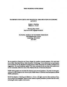
Figure 1. A network of place cells created by the Gerstner-Abbott model (figure reproduced from Gerstner & Abbott, 1997). Pointers arise from place cell receptive field shifts, and indicate the target’s direction, taking walls and obstacles into account.
the center of each place cell’s receptive field increases, the cell’s response falls off according to a Gaussian function. These receptive fields overlap such that several place cells will respond in parallel when the model is at a particular location in the environment. When multiple cells are active at the same time, the model’s location is encoded as a weighted function of the center of the mass of active cells, taking into account the difference in activity across cells. Initially, the encoded location corresponds to the actual spatial location of the model. As the model explores the environment randomly, the receptive field of each place cell is tuned according to a Hebbian learning rule. The result is a shift in encoded location away from walls and obstacles, toward one or more targets in the environment. The inconsistency between the physical spatial location of the model and the place cell-encoded location provides a pointer which can be used to generate a path to a target. The place cell network of the Gerstner-Abbott model may be thought of as a type of cognitive map of the environment. Instead of encoding spatial information per se, the shift in place cell receptive fields encode navigation paths, which provide pointers to the target from arbitrary locations in the environment. Figure 1 illustrates the receptive field shift for a simple sample environment. Discussion. The Gerstner-Abbott model makes several simplifying assumptions which are unrealistic for a model of human spatial navigation. The model explores its environment randomly, moving in straight-line paths until being deflected by a wall or obstacle. Although random exploration is justifiable in the context of this highly-simplified model, navigation data from human subjects, as presented in Section Two of this thesis, show that human navigation is highly efficient. Therefore, a more complete model of human navigation should make use of a non-random foraging strategy.
MODELING HUMAN SPATIAL NAVIGATION
3
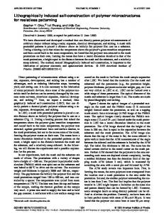
Figure 2. (a.) Place and view graph created by the Sch¨ olkopf-Mallot model, with places pi (i = 1, ..., 7) and views vj (j = 1, ..., 12). (b.) Associated directed place graph with corridors cj corresponding to views vj . An optimal path may be generated between any vertices in the place graph. Figures reproduced from Sch¨ olkopf & Mallot (1995).
The inspiration for the Gerstner-Abbott model is a hungry animal scavenging for food. As such, the learning mode is triggered by a food-based reward system. Learning via receptive field tuning occurs when the animal is looking for food. Once the animal has eaten, this learning mode shuts off. The authors suggest that an attention-activated learning mode might replace (or augment) the food-based reward system in a more general model. In the context of the experiments presented in Section Two, an attention-activated learning mode would imply that the learning mode was constantly activated, since subjects are always looking for either a new passenger or a target store in the virtual environment. This suggests that environment learning should take place both while searching for a passenger and while seeking a target store. Sch¨ olkopf-Mallot Directed View Graph Model Sch¨olkopf & Mallot (1995) propose a model which uses a graph representation of mazelike environments. Views at particular locations are stored at vertices.1 Branches, which join adjacent vertices, represent temporal relationships between views. This view graph is built as the model explores. At first, exploration is random, but as an exploration matrix (which stores locations in the maze that have been visited) is filled in, the model tends toward unexplored regions. Information about paths between arbitrary locations in the maze can be extracted from the view graph, regardless of whether the paths have previously been traversed. In some 1
A vertex is the point at which two branches of a graph meet. For a concise introduction to graphs and graph theory, see Storer (2002).
MODELING HUMAN SPATIAL NAVIGATION
4
cases, empty cells in a view graph’s adjacency matrix2 can be filled in as “expected” views, using existing local views and associations between them. A place graph, which represents relationships between locations in the maze, may be extracted from the view graph. The place graph may be used to find a path between two arbitrary locations. Provided that the model has explored enough of the environment, the path will be optimal (the shortest possible path). In a 12-view maze (see Figure 2), 110 steps are enough to generate all possible shortest paths between all points in the maze. (See Sch¨olkopf & Mallot (1995) for more statistics regarding shortest path versus learning time.) Discussion. The model’s view graph provides enough information to generate optimal paths between environment locations. In this way, a cognitive map representing the spatial layout is not explicitly needed to navigate an environment. This finding is useful, but may not be universal, since there are a discreet number of possible moves in a maze environment, whereas there are a potentially infinite number of moves in an open environment. The virtual environments presented in Section Two are open environments, since the number of possible views is infinite for all practical purposes. Nevertheless, these environments may be approximated by place and/or view graphs, where each intersection is represented by a vertex and each road is represented by a branch. In order to simplify complex open environments, it is sometimes useful to find a maze-like approximation. In order to simplify path generation and view computations, my ideal navigator model navigates a graph-like approximation of the virtual town. The mechanisms underlying goal path generation are left out of the Sch¨olkopf-Mallot model. It is shown only that it is possible to generate an ideal path connecting two points, given the view graph, using a brute force algorithm in which many paths are tested. Given that human subjects in Experiments One and Two were observed to generate goal paths quickly and efficiently, it is unlikely that they employed a brute force technique. The exploration strategy implemented by the Sch¨olkopf-Mallot model attempts to build up the exploration matrix quickly by tending toward unexplored locations. In my ideal navigator model, I add to this by having the model explore nearby unexplored locations before far away unexplored locations. In this way, the goal-directed ideal navigator attempts to minimize the goal path distance by avoiding “zig-zags” back and forth between noncontiguous unexplored patches. Voicu’s Hierarchical Cognitive Map Model Voicu (2003) presents a model based on a hierarchical cognitive map, in which spatial information is organized in three networked layers of varying resolution, which are built up as the model explores (see Figure 3a). Initially, exploration is random. The model assigns a unique code to each landmark for encoding associations. As the model explores, associations are strengthened between all landmarks which are either currently perceived or currently in the model’s working memory. As associations are strengthened, the exploration strategy adapts so that previously encoded landmarks are avoided. Once the cognitive map contains associations between at least ten landmarks, the model changes its exploration strategy such that it tends toward landmarks with the fewest associations. 2
An adjacency matrix is a tabular representation of all edges in a graph.
MODELING HUMAN SPATIAL NAVIGATION
5
The lowest layer of the hierarchy is the most detailed, containing associations between all encoded landmarks. Once the lowest layer is in place, the second layer is constructed. Initially, the second layer is assigned landmarks from the first layer whose associations are strongest. Associations between these landmarks are constructed using information from the first layer. Each of the landmarks, l, in the second layer are activated; this activation spreads according to existing associations, until the total activity is bounded by a set range. If the last landmark to be activated with strength s is x, the association between l and x is assigned strength s. Similarly, the third layer is constructed from the second layer using the second layer landmarks with the strongest associations. If all landmarks in the second layer have equally strong associations, no third layer is constructed (see Figure 3b). Interactions between the three layers allow for complex representations of clusters of landmarks in working memory. In order to generate a path to a goal landmark, the goal landmark is activated in the cognitive map. The activation spreads until it reaches the model’s current location. The model simply follows the activation gradient to the goal from its current position. Landmarks closer to the goal will have greater activation. Discussion. This model’s hierarchical cognitive map is useful for large environments with many landmarks, but becomes impractical (or redundant) for smaller environments such as those presented in Section Two. In addition, the detailed, multi-step foraging strategy is more focused on obtaining a detailed representation of the environment than locating a target within the environment quickly or efficiently. A realistic model for human navigation in a goal-directed task (in which navigators are motivated to perform quickly) might sacrifice a layered hierarchy for a less robust (but faster to build) flat cognitive map.
Virtual Reality as an Experimental Paradigm Desktop virtual reality has been popularized over the last decade with hit video games such as DOOM, Quake3 , and Unreal Tournament4 . In recent years, it has become possible to construct custom-built virtual reality games using open source tools. The high level of configurability implied by custom-built games makes them ideal for experimentation. The discovery that navigationally-useful cells are activated during a virtual reality navigation task (Ekstrom et al., 2003) presumably implies that subjects treat virtual navigation similarly to real-world navigation. In fact, performance is significantly degraded if the illusion of natural movement is taken away, for example by reducing the rate of optic flow (Kirschen et al., 2000). In the remainder of this thesis, I describe two virtual reality experiments in which subjects play taxicab drivers in a small town. For each delivery I define an ideal path distance, which approximates the shortest delivery path possible. The difference between the ideal path and the observed delivery path is called the excess path length, and may be used as a performance metric (this approach was used in Newman et al., 2005). Recently, ideal performers have been used as benchmarks for behavioral data (RoblesDe-La-Torre & Sekuler, 2004). Behavioral data from Experiment One suggest that subjects themselves are behaving as ideal navigators. I present an ideal navigator model which 3 4
DOOM and Quake are trademarks of idSoftware. Unreal Tournament is a trademark of Epic Games
MODELING HUMAN SPATIAL NAVIGATION
6
(a)
(b)
Figure 3. Voicu’s hierarchical cognitive map representation of an environment. Figures reproduced from (Voicu, 2003). (a) Landmarks are represented by circles. Thin lines represent first-layer connections. Medium lines represent second-layer connections. Thick lines represent third-layer connectios. (b) Landmarks are represented by the numbers 1 through 30. On the left, solid lines indicate layer one connections and dashed lines indicate layer two connections; there are no layer three connections. On the right, the layers are organized as an ordered tree.
MODELING HUMAN SPATIAL NAVIGATION
7
explores efficiently and learns the environment layout quickly. For Experiment One, the ideal navigator correctly predicts excess path length for between 60 and 70 percent of the deliveries made. In Experiment Two, size of the virtual environment is increased by 41%, effectively increasing spatial memory demands on subjects. In this larger environment, the ideal navigator is only able to predict excess path length of between 40 and 50% of the deliveries. This suggests that a critical component responsible for subject performance is missing from the ideal navigator model. After adjusting assumptions about the ideal navigator’s vision and memory, the model is able to account for mean performance observed in both experiments.
Materials and Methods Experiment One Newman et al. (2005) present a desktop virtual reality paradigm,5 in which subjects play taxicab drivers in a small town. During a testing session subjects picked up and delivered passengers in two environments. Random assignment to one of five conditions determined the similarity of the first environment to the second environment. For the purposes of this thesis, I am concerned only with the first environment tested.6 Because my proposed model does not take into account learning across conditions, it only makes sense to look at environments which have not been seen before. Subjects One hundred twenty-one Brandeis University undergraduates (59 males, 56 females)7 participated for monetary compensation with an additional performance-based bonus. Construction of Virtual Towns Each virtual town was laid out on a 5 × 5 orthogonal grid of roads, with one uniquelytextured landmark centered on each block. Twenty-one of these landmarks were buildings, which varied slightly in width and greatly in height. Buildings were surrounded by lawn to prevent subjects from driving up to them. The remaining four blocks contained stores, which were of equal size, and were surrounded by pavement. Deliveries were always made to stores. The outer boundary of the town was marked by a texture-mapped stone wall; no other visual information could be seen beyond the boundary. Each block was surrounded by drivable road. If the road is taken to be one virtual unit wide, each block measured 2 × 2 virtual units, and the environment measured 16 × 16 virtual units. Each building occupied approximately one block (4 square units) at its base, while each store occupied a 0.7 × 0.7 × 0.35 unit rectangular prism. Of the 256 square units occupied by the environment, 100 were covered by blocks containing landmarks, and 156 were covered by drivable road. Before the start of the subject’s session, the landmarks 5 A similar version of this paradigm is discussed in earlier work (see Caplan et al., 2003; Ekstrom et al., 2003). 6 Newman et al. (2005) refer to this condition as Experiment Two, Environment One. 7 Gender data for 8 of the subjects were not recorded.
MODELING HUMAN SPATIAL NAVIGATION
8
Figure 4. Experiment One: Sample layout for a randomly generated town. Buildings are shown in black; stores are shown in red. Roads, shown in white, surround each block. Note: this figure is not drawn to scale.
chosen to occupy each block were randomly selected and arranged, with the constraint that no two stores could be found in adjacent blocks. A sample layout is shown in Figure 4. Navigation and Gameplay Subjects controlled the virtual taxicab using the four arrow keys (↑, ↓, ←, →) on a standard 101-key keyboard. If more than one key was pressed, only the most recent key press would apply. The turning rate was 20◦ /sec, and driving speed was constant at 1.17 units/sec. The screen was refreshed every 30 msec. The field of view was set to 56◦ with a screen resolution of 640 × 480 pixels. During gameplay, subjects picked up and delivered twenty passengers. The session was block-random, such that each of the four stores were delivered to before the next round of deliveries began. Passenger placement was pseudo-random, with the constraint that a passenger could not be in the direct line of sight of the previous goal. Each delivery began with a foraging path, during which the subject located the next passenger. When the passenger was picked up, a text screen notified the subject of the next target store. The delivery path started with picking up the passenger and ended at the goal (the passenger’s destination store). Each subject navigated twenty foraging paths and twenty delivery paths during their session. Subjects began with $300 of virtual cash. For each 10 sec spent moving or turning, subjects were docked $1, with the restriction that a maximum of $1 could be docked for any continuous period of standing still. Upon successfully completing a delivery, subjects were rewarded $50 virtual cash. The current earnings were continuously displayed in the upper right corner of the screen. The upper left corner of the screen contained a short description of the current instructions (e.g., “Find a passenger” or “Find the Java Zone”). A screen capture from a typical foraging path is shown in Figure 5.
MODELING HUMAN SPATIAL NAVIGATION
9
Figure 5. Experiment One: Screen capture taken during a typical foraging path. The autopac store and several buildings are visible.
Procedure Subjects were given a small delivery practice task in order to familiarize them with gameplay. The practice environment measured 3 × 3 blocks, with a store in each of the four corner blocks. There were no buildings in the practice environment. During the practice session, subjects picked up four passengers and delivered them to each of the four stores. Store textures used during the practice session were not re-used in the main task. After the first practice task, images of stores the subject would encounter later in their session were displayed on screen along with the store name. Subjects were asked to read the store names aloud. The list of stores was presented four times, each time in a new random order. The purpose of the second practice task was to familiarize subjects with the appearance of stores before entering the town. During the practice tasks, the experimenter remained in the testing room, and answered any questions unrelated to strategy. After the practice tasks were complete, the experimenter left the room, and subjects were assigned a 5 × 5 town. Measuring Performance Excess path length is defined as the difference between the delivery path distance and the ideal path distance. The ideal path distance is equal to the city block distance (∆x+∆y) from the passenger to the goal store. Mean excess path length decreases as a function of delivery number, as shown in Figure 6a. Although excess path length provides a rough estimate of performance, it fails to take into account the relative efficiency of paths of different lengths. Let us suppose that there
MODELING HUMAN SPATIAL NAVIGATION
10
3
Excess Path Length (blocks)
2.5
2
1.5
1
0.5
0
0
5
10 Delivery
15
20
15
20
(a)
1.8 1.7
Percent Deviation
1.6 1.5 1.4 1.3 1.2 1.1 1
0
5
10 Delivery
(b)
Figure 6. Experiment One: (a) Mean excess path length. Subjects improve with the number of deliveries made. Error bars represent ± 1 s.e.m. (b) Percent deviation from ideal path distance. Subjects improve with the number of deliveries made. Error bars represent ± 1 s.e.m.
11
MODELING HUMAN SPATIAL NAVIGATION
are two deliveries, a and b, for which the excess path length is one block. For delivery a, suppose that the ideal path distance is ten blocks. For delivery b, the ideal path distance is only two blocks. Clearly, delivery a is more efficient than delivery b. However, according to the excess path length measure, the performance for both deliveries is considered to be equal. Percent deviation of a delivery path is defined as the ratio of the delivery path distance 11 to the ideal path distance. For example, delivery a has a percent deviation of 10 = 1.1, 3 and delivery b has a percent deviation of 2 = 1.5. Thus, delivery a is considered to exhibit better performance than delivery b. Percent deviation from the ideal path distance is shown to decrease (improve) as a function of delivery number in Figure 6b. Unfortunately, the percent deviation measure is not necessarily preferential to the excess path length measure in all situations. The reason for this is due to an oversimplification of the ideal path distance measure. Let us suppose a passenger and goal are placed as shown in Figure 7. According to the ideal path distance measure, the passenger is three blocks away from the goal. However, given that there are several buildings blocking a direct path to the goal, the driver must “swerve” around the buildings before reaching the goal store. The distance of the swerve is fixed, so the excess path length is constant (assuming that the driver swerves consistently). Notice that the total path distance required to make the delivery changes as a function of the number of buildings separating the passenger and goal. In this way, percent deviation becomes a measure of environment constraints rather than a true measure of performance. In the following table, I assume a one-block swerve is necessary to circumvent any relevant obstacles:
Ideal path distance: Path Efficiency: Excess Path Length:
1 2/1 = 2 1
2 3/2 = 1.5 1
3 4/3 = 1.33 1
4 5/4 = 1.25 1
5 6/5 = 1.2 1
Despite their inconsistencies in specific cases, it should be noted that for Experiment One data excess path length and percent deviation are correlated (correlation coefficient = 0.9593). This suggests that either metric should perform relatively well in the majority of delivery paths. Probability of getting lost is defined as the proportion of paths which are worse (according to a pre-defined performance metric) than a threshold percentile. First, all observed delivery paths are ranked by excess path length or by path efficiency. A threshold percentile (e.g., 95%) is chosen; all deliveries ranked worse than the threshold percentile are tagged. Therefore, the probability of getting lost is equal to the proportion of tagged paths in each condition. The probability of getting lost measure reveals trends in the data, rather than performance for individual paths (Figure 8). When attempting to predict performance for individual deliveries, a stochastic component of exploration begins to pervade, as will be seen in the modeling section of this thesis. The probability of getting lost measure can be useful as a means of containing the resulting noise.
MODELING HUMAN SPATIAL NAVIGATION
12
Figure 7. Swerving around a building. When the start position of the passenger is directly aligned with the goal in either the horizontal or vertical direction (but is not directly adjacent to the goal) the driver must swerve around one or more landmarks in order to make the delivery. In these cases, the optimal path will have an excess path length equal to the city block distance from the passenger to the nearest intersection.
0.25
p(LOST)
0.2
0.15
0.1
0.05
0
0
5
10 Delivery
15
20
Figure 8. Experiment One: probability of getting lost. Error bars represent ±1 s.e.m.
MODELING HUMAN SPATIAL NAVIGATION
13
Efficient Navigation Because passenger placement is random, it is impractical for subjects to memorize delivery path routes.8 Instead, the rapid learning observed in this task may be due to the building of a cognitive map which stores layout information for known locations in the town. As the cognitive map becomes more detailed, subjects are able to utilize remembered layout information to synthesize efficient delivery paths from arbitrary passenger pickup locations to known stores. As shown in Figure 9, observed distributions of excess path length are highly skewed toward zero. These findings provide motivation for the creation of an ideal navigator model as a means of predicting excess path length (see Section Three). The ideal navigator, which models performance of the perfect subject, will generate an optimal path (excess path length = 0) unless either (a) the current goal has not yet been displayed on screen, or (b) environment constraints require swerving around obstacles in order to complete the delivery (as in Figure 7). In this way, the ideal navigator provides a more realistic optimal performance benchmark than ideal path distance, since the ideal navigator operates according to similar movement constraints as the subject (see Robles-De-La-Torre & Sekuler, 2004).
Experiment Two Subjects in Experiment One learned their environments quickly, making it difficult for the researchers to learn about errors in spatial memory. As originally reported by Korolev (2005), participants in Experiment Two were tested in a 41% larger environment than in Experiment One. In addition, the paradigm underwent several feature upgrades and cosmetic changes (see Figure 10) aimed at increasing perceived realism during gameplay. Subjects were tested over the course of three sessions (each separated by at least one day), during which they made deliveries to three towns in the following order: A: A new town that had never been seen before B: A second town that had never been seen before A0 : A third town which was identical to town A For the purposes of this thesis, I am concerned only with each unique town navigated. All A0 environments were ignored in my analysis and modeling (see Korolev (2005) for a description of the A0 condition and its implications). Because my proposed model does not take into account learning across conditions, it only makes sense to look at environments which have not been seen before. Subjects Twenty-one9 Brandeis University and University of Pennsylvania students and staff (12 male, 9 female) participated for monetary compensation, with an additional bonus based on performance. 8 In larger environments, “route memorization” may be useful between known hubs, as suggested by Voicu’s hierarchical cognitive map model (Voicu, 2003). However, for the simple, highly regular environments used in this experiment, a hierarchical representation becomes redundant. 9 Seven new subjects were tested after data from fourteen subjects were reported by Korolev (2005) and Mollison (2005).
MODELING HUMAN SPATIAL NAVIGATION
14
70
60
Number of Subjects
50
40
30
20
10
0
0
2
4
6 8 10 12 Excess Path Length (Blocks)
14
16
(a) Delivery One
70
Number of Subjects
60 50 40 30 20 10 0
0
5 10 Excess Path Length (Blocks)
15
(b) Delivery Two
Figure 9. Experiment One: excess path length distribution for delivery one (a) and two (b). The distributions are skewed toward an excess path length of zero.
MODELING HUMAN SPATIAL NAVIGATION
15
Figure 10. Experiment Two: Screen capture taken during a typical foraging path. The Butcher Shop store, a passenger, and several buildings are visible.
Construction of Virtual Towns Virtual towns were constructed similarly to those in Experiment One. Experiment Two towns were laid out on a 6 × 6 block orthogonal grid of roads surrounded by an outer wall. The dimensions of the town may be expressed as 19 × 19 virtual units, where the width of the street is one virtual unit, and where each block occupies 2 × 2 virtual units. Of the 361 square virtual units, 144 are occupied by landmarks, 31 of which are buildings and 5 of which are stores. As in Experiment One, buildings occupied approximately 4 square units at their base, but varied greatly in their height. Stores occupied a 0.7×0.7×0.35 rectangular prism. At the start of each session, a small 3 × 3 practice environment (one store in each corner) and two full size 6 × 6 environments were randomly generated such that no store texture was repeated. Stores were placed pseudo-randomly with the constraints that (a) no two adjacent blocks could each contain stores, (b) all four corners of the environment could not each contain a store, (c) no row or column could contain all stores, and (d) neighboring stores were required to have at least two buildings between them in both the horizontal and vertical directions. These constraints meant to slow learning of the town layout relative to Experiment One. Navigation and Gameplay Subjects controlled the virtual taxicab using a USB10 gamepad controller with a 360◦ directional pad. Driving speed was modulated by the pressure exerted on the pad, with a 10
Universal Serial Bus
MODELING HUMAN SPATIAL NAVIGATION
16
maximum driving speed of 1 unit/sec. The turning rate was 50◦ /sec. The field of view was set to 60◦ with a screen resolution of 800 × 600 pixels, and was refreshed every 20 msec. During gameplay, subjects picked up and delivered fifteen passengers per environment. The goals chosen were block-randomized, such that each of the five stores were delivered to before the next round of deliveries began. Passenger placement was pseudo-random, with the constraints that no two passengers could occupy the same block, and that a passenger could not be in the direct line of sight of the previous goal. Six potential passengers were placed at the start of each delivery. When the passenger was picked up, a text screen notified the subject of the next target store. The delivery path begins when the passenger is picked up, and ends at the goal store. For the first delivery in each new environment, a passenger was placed directly in front of the subject. Each subsequent delivery began with a foraging path, during which the subject located the next passenger. By starting subjects with a passenger, the first foraging path is effectively eliminated. Performance during the first delivery becomes highly dependent on the subject’s foraging strategy, since the subject has no prior exposure to the environment. Nevertheless, for 18.25% of first deliveries in previously unseen environments, subjects still manage to generate optimal paths (excess path length = 0). I attribute optimal performance during the first delivery simply to luck. Initially subjects began with 300 points. Upon successful delivery, subjects were rewarded 50 points, but were docked 1 point for every three seconds of gameplay. The score was continuously displayed in the upper right corner of the screen. The upper left corner of the screen contained a short description of the current goal (e.g., “Find a passenger” or “Find the Coffee Store”), as in Experiment One. A typical view seen during a subject’s foraging path is shown in Figure 5. Procedure Subjects were given a small delivery practice task in order to familiarize them with picking up and dropping off passengers. The practice environment measured 3 × 3 blocks, with a store in each of the four corner blocks. There were no buildings in the practice environment. During the practice session, subjects picked up four passengers and delivered them to each of the four stores. Store textures used during the practice session were not re-used in the main task. After the first practice task, images of stores the subject would encounter later in their session were displayed on screen along with the store name. Subjects were asked to read the store names aloud. The list of stores was presented four times, each time in a new random order. The purpose of the second practice task was to familiarize subjects with the appearance of stores before entering the town. After the practice tasks were complete, the subjects were assigned a 6×6 town. Subjects picked up and delivered fifteen passengers (A condition). At the end of the fifteenth delivery, subjects were allowed to take a short break, leaving the testing room if desired. After an additional showing of the store familiarization task, subjects were given a second town (B condition), followed by a break after fifteen deliveries. After a third showing of the store familiarization task, subjects made fifteen deliveries in their last environment (A0 condition). In subsequent sessions, the initial practice environment was omitted, but otherwise testing procedure was identical.
17
MODELING HUMAN SPATIAL NAVIGATION
10 9
Excess Path Length (Blocks)
8 7 6 5 4 3 2 1 0
0
1
2 3 4 5 Number of Unique Environments
6
7
Figure 11. Experiment Two: First delivery excess path length as a function of (unique) environment number. Error bars represent ±1 s.e.m.
During the testing session, the experimenter remained in the testing room, and answered any questions unrelated to strategy. Learning Across Environments Subjects in Experiment Two make deliveries in six unique environments. Subjects appeared to improve slightly as a function of the number of unique environments experienced (see Figure 11), however this improvement was not statistically significant.11 In order to increase the size of the data set for analysis and modeling purposes, I grouped data from all environments together. Results Performance for Experiment Two was analyzed using excess path length, percent deviation measure, and probability of getting lost (Figure 12). As in Experiment One, delivery performance improves as subjects gain experience delivering passengers in the town.
Model My attempt to model human spatial navigation led me to construct two computational models. The first is an ideal navigator which generates an optimal delivery path when a goal store has previously been seen. When the goal store has not been seen, the ideal navigator forages efficiently to find the goal quickly. The second model, nicknamed Magellan,12 11 I performed a right-tailed two-sample T-test comparing the first deliveries of environments one and six, assuming equal variance (p = 0.1429). 12 Ferdinand de Magellan was the first person to circumnavigate the globe (1519 - 1522). Professor Robert Sekuler unofficially named the degraded ideal navigator after Magellan in an email correspondence with the author dated 6/6/2004.
MODELING HUMAN SPATIAL NAVIGATION
18
8
Excess Path Length (Blocks)
7 6 5 4 3 2 1 0
0
2
4
6
8 Delivery
10
12
14
16
14
16
14
16
(a) Excess Path Length 5 4.5
Percent Deviation
4 3.5 3 2.5 2 1.5 1
0
2
4
6
8 Delivery
10
12
(b) Percent Deviation
0.25
p(LOST)
0.2
0.15
0.1
0.05
0
0
2
4
6
8 Delivery
10
12
(c) P (LOST )
Figure 12. Experiment Two: A variety of performance measures. Error bars represent ±1 s.e.m.
MODELING HUMAN SPATIAL NAVIGATION
19
systematically degrades the memory and vision of the ideal navigator in order to account for subject error.
Defining An Optimal Path When the excess path length is zero, we say that the delivery path is optimal. However, in some cases when the excess path length is greater than zero, the delivery path may still be optimal. One such situation is described in Section Two and illustrated in Figure 7. When the start position of the passenger is directly aligned with the goal (in either the horizontal or vertical direction), but is not directly adjacent to the goal, the driver must swerve around one or more landmarks in order to make the delivery. In these cases, the optimal path will have an excess path length equal to the twice the city block distance from the passenger to the nearest intersection (once for a swerve in the beginning of the path and once for a swerve at the end of the path).
Ideal Navigator Model An ideal navigator (a) sees all landmarks displayed on screen and (b) remembers their allocentric spatial location without noise or forgetting. The model (c) uses this information to generate optimal delivery paths to goal stores which have been seen previously. For goals which have not yet been seen, the ideal navigator (d) implements an efficient foraging algorithm which quickly searches unknown sections of the town. As soon as the goal is located, an optimal path is generated to it from the model’s current location. I define one step of the model to be a move from one intersection in the town to an adjacent intersection. Consequently, the model’s heading will always be a multiple of 90◦ . This simplification allows me to focus on path distance - rather than the exact shape of a particular delivery path - as an indirect measure of spatial knowledge of the environment. Constraining the model’s movement in this way means that the model can never out-perform the ideal path. As the model steps, we compute which landmarks are visible along that step in the corresponding virtual environment. Each visible landmark is mapped onto the model’s internal representation of the environment, which includes a spatial location and a unique identifier for each landmark. Initially, the model’s internal representation is empty. Simplifying the Delivery Path During the experiments, the only constraint placed on subjects is that they must drive on the road (not on the sidewalk or grass). Because the roads are relatively wide, subject paths within the roadway may take complicated zig-zags and turns. An important implication of this freedom of movement is that subjects can out-perform the ideal path as I define it. While the ideal path length is computed using the city block distance (the sum of two legs of a right triangle), the subject’s delivery path has the ability to cut corners at headings other than 90◦ . Thus, the true ideal subject path is actually somewhere between the city block distance and the Euclidean distance from passenger to goal. In order to make a fair performance comparison between subjects and the model, I must guarantee that subjects can never perform better than the ideal path. Thus, from here on, I use a simplified version of the subject’s path, computed as follows:
MODELING HUMAN SPATIAL NAVIGATION
20
1. An n × m environment is divided into a (3n + 1) × (3m + 1) grid13 of equal total dimensions. This means that if the n × m environment spans 256 virtual square units, the (3n + 1) × (3m + 1) grid will span 256 virtual square units as well. 2. The subject’s path is plotted on the (3n + 1) × (3m + 1) grid. 3. Each point along the subject’s path is rounded to the center of its block. 4. Rounded points are connected. Because the town is laid out on an orthogonal grid, the heading along the simplified path is always a multiple of 90◦ . Figure 13 demonstrates the effects of path simplification on the excess path length performance metric. Ideal Navigator Concerns Several difficulties arise when attempting to model a succession of deliveries in a given environment. First, the foraging path distance varies from subject to subject, since passenger placement is random. In addition, subjects may have different foraging strategies which may change as the subject learns their environment. The specific strategy subjects are using at a given point during their session is extremely difficult to infer from behavioral data, especially given that individual deliveries may be noisy. Even when the model predicts the correct observed delivery path distance, the particular shape of the model’s path may differ from the subject’s simplified path. For a given delivery requiring ∆x horizontal moves and ∆y vertical moves, the total number of unique paths of equal length is (∆x+∆y)! ∆x!∆y! (see Appendix A for further explanation). If left uncorrected, the model would have access to landmark information for landmarks which were never actually displayed on the subject’s screen. As the model makes more deliveries, these errors propagate, and the model’s session diverges from the subject’s session. I overcame these difficulties by erasing the model’s memory when each new passenger is picked up. The model’s memory is then replaced with all landmarks actually seen from the start of the subject’s session until the moment at which the passenger is picked up. When the model’s memory is guaranteed to contain only landmarks displayed on the subject’s screen, we say that the model’s memory is synchronized with the subject’s memory. Ideal Navigator Algorithm From the time the passenger is picked up until the time the model arrives at the goal, the model’s algorithm may be summarized by two instructions: 1. Find a sub-goal. The sub-goal is equal to the goal (the passenger’s intended destination) if the location of the goal is known. Otherwise, set the next subgoal to be the nearest block not yet associated with a landmark. If there are multiple sub-goals, choose randomly between them. This step implements the ideal navigator’s efficient foraging strategy. 2. Take a step toward the sub-goal. If there are multiple possible directions to step, choose randomly between them. 13
Recall that each block is twice as wide as the road, so the total width of a road-block pair is three road-widths.
21
MODELING HUMAN SPATIAL NAVIGATION
Excess Path Distances vs. Number of Deliveries 3 Subjects Subjects (Simplified) 2.5
Excess Path Distance (Blocks)
2
1.5
1
0.5
0
−0.5
0
5
10 15 Number of Deliveries
20
25
(a) Experiment One
8 Subjects Subjects (Simplified)
Excess Path Length (blocks)
7 6 5 4 3 2 1 0
0
2
4
6
8 Delivery
10
12
14
16
(b) Experiment Two
Figure 13. Excess path length vs. number of deliveries for Experiment One (a) and Experiment Two (b). Subject performance (blue) is measured by comparing the average goal path distance to the average ideal path distance, for each delivery made. To compute the simplified subject excess path length (black), we first round all positions to the nearest intersection. In this way, the simplified paths consist of straight lines and 90◦ turns. Note that while the actual excess path length can be negative, the simplified excess path length is non-negative. Error bars represent ±1 s.e.m.
MODELING HUMAN SPATIAL NAVIGATION
Delivery 1
Delivery 2 15 Observed
Observed
15 10 5 0
0
5
10 Predicted Delivery 3
5
0
5
10 Predicted Delivery 4
15
0
5
10 Predicted
15
15 Observed
Observed
10
0
15
15 10 5 0
22
0
5
10 Predicted
15
10 5 0
Figure 14. Experiment One: observed excess path length (blocks) vs. predicted excess path length, using the ideal navigator. Note that many data points overlap at (0, 0). In order to disambiguate this overlap, a small amount of random noise is added to the plot in order to jitter data points.
Because a step always brings the model one block closer to the sub-goal, the modeled path is by definition optimal. When the passenger’s destination has been encoded in the model’s memory, the initial sub-goal is equal to the passenger’s destination, and so the model generates an optimal delivery path. When the passenger’s destination is unknown, we implement an efficient foraging strategy by setting the sub-goal to the center of the nearest block on which no landmark has been previously seen. In this way, sub-goals are chosen to be near each other, and so nearer locations will be explored before far locations. As a result, the model will waste fewer steps traveling back and forth across the environment, minimizing effort and time per delivery (Robles-De-La-Torre & Sekuler, 2004). Although I claim that the ideal navigator’s strategy is ideal, it is possible for subjects to “beat the ideal navigator.” This seems counter-intuitive, since the ideal navigator should make optimal use of all information available to the subject. However, when there is a lack of information about the goal, there is a stochastic component to the shape of the delivery path. This means that there is some chance of navigating to the location of the goal without actually ever having seen it. This “luck” component becomes significant in the first few deliveries, when only a small portion of the environment has been explored (and so the foraging stochastic component plays a large role in the foraging path). Once all landmarks in the environment have been seen, the ideal navigator should either match or outperform subjects14 in every delivery. Figure 14 plots observed excess path length versus predicted excess path length for the first four deliveries of Experiment One. Note that many data points overlap near the origin. The corresponding plot for Experiment Two is shown in Figure 15. As illustrated in Figure 16, the number of subjects outperforming the ideal navigator drops to zero after the first delivery. This differs from Experiment One, in which subjects are given an opportunity to explore before picking up their first passenger. In addition, the larger town size in Experiment Two means that its layout will require more steps to fully 14
Simplified subject path.
MODELING HUMAN SPATIAL NAVIGATION
Delivery 2
50
50
40
40
Observed
Observed
Delivery 1
30 20 10
30 20 10
0
0
20 40 Predicted Delivery 3
50
50
40
40
Observed
Observed
0
30 20 10 0
23
0
20 40 Predicted Delivery 4
0
20 40 Predicted
30 20 10
0
20 40 Predicted
0
Figure 15. Experiment Two: observed excess path length (blocks) vs. predicted excess path length, using the ideal navigator. Note that many data points overlap at (0, 0). In order to disambiguate this overlap, a small amount of random noise is added to the plot in order to jitter data points.
explore. Thus, in Experiment Two, the stochastic foraging component leaks into the second delivery. Ideal Navigator Results Given the relatively small 5 × 5 town (256 virtual square units) of Experiment One, the ideal navigator predicts the observed excess path length an average of 66.6% of the time. Experiment Two, with a 6 × 6 town (361 virtual square units), represents a 41% increase in environment size. A corresponding drop in performance is observed, and so the ideal navigator’s ability to predict subject performance is diminished, as shown in Figure 17. The particular percentage of deliveries predicted by the ideal navigator is less important than the drop in ability to fit the data in the larger town of the second experiment. The decreased portion of subject delivery paths explained by the ideal navigator in Experiment Two are suggestive of two ideas. First, the ideal navigator must be discounting one or more key factors underlying delivery performance. Second, these factors must play a more significant role in determining performance in Experiment Two, which implies their effectiveness is related to environment size. Predicting Environment Difficulty. Although the ideal navigator model uses a consistent foraging strategy for each randomly generated environment, its ability to generate optimal delivery paths varies. This suggests that some environments may be more difficult than others. The ideal navigator’s delivery performance can be used as a metric for environment difficultly as follows (this is done separately for each delivery): 1. Pair each subject’s observed excess path length with the model’s predicted excess path length for that delivery. 2. Order all pairs based on the model’s predictions. 3. Divide the ordered data into n equally sized bins. 4. Define a threshold percentile, θ, beyond which subjects are considered to be “lost” while making their delivery.
24
MODELING HUMAN SPATIAL NAVIGATION
0.5 0.45
p(predicted > observered)
0.4 0.35 0.3 0.25 0.2 0.15 0.1 0.05 0
0
5
10 Delivery Number
15
20
(a) Experiment One
0.5 0.45
p(predicted > observered)
0.4 0.35 0.3 0.25 0.2 0.15 0.1 0.05 0
0
2
4
6
8 10 Delivery Number
12
14
16
(b) Experiment Two
Figure 16. Probability of beating the ideal navigator as a function of delivery number. (a) During the first delivery of Experiment One, some subjects may guess the direction of the goal without having previously seen it. After the first delivery, the ideal navigator consistently matches or out-performs all subjects. (b) After the second delivery of Experiment Two, the ideal navigator consistently matches or out-performs all subjects. Recall that there is no foraging path for the first delivery in Experiment Two.
25
MODELING HUMAN SPATIAL NAVIGATION
1 0.9
p(predicted = observered)
0.8 0.7 0.6 0.5 0.4 0.3 0.2 0.1 0
0
5
10 Delivery Number
15
20
(a) Experiment One
1 0.9
p(predicted = observered)
0.8 0.7 0.6 0.5 0.4 0.3 0.2 0.1 0
0
2
4
6
8 10 Delivery Number
12
14
16
(b) Experiment Two
Figure 17. Ideal Navigator: Correct Predictions. Probability of having excess path length predicted by the ideal navigator as a function of delivery number. Error bars represent ±1 s.e.m. (a) Experiment One: In delivery one, the model’s predictive power is low due to a stochastic foraging component. The mean probability of predicting the correct excess path length is 66.6%. (b) Experiment Two: In deliveries one and two, the model’s predictive power is low due to a stochastic foraging component. The mean probability of predicting the correct excess path length is 42.8%.
MODELING HUMAN SPATIAL NAVIGATION
26
5. Set q equal to the excess path length observed for the subject in the θ th percentile. 6. For each of the n bins, compute the fraction of subjects with an excess path length greater than or equal to q. For the first delivery of Experiment One, and the first two deliveries of Experiment Two, this metric performs poorly. As noise due to stochastic foraging decreases in later deliveries, the ideal navigator is able to successfully rank environments as easy, medium, or difficult (Figure 18.) Ideal Navigator Shortcomings The ideal navigator accounts for errors due to lack of information, but does not account for human errors due to inattention (failure to encode a landmark displayed on screen) or forgetting over time (failure to recall a previously encoded landmark). In Experiment One, the ideal navigator model does a fairly good job of explaining observed performance (Figure 17a). However, as the size (and therefore complexity) of the environment is increased in Experiment Two, the ideal navigator fails to account for over half of the delivery paths made (Figure 17b). Because the distributions of excess path length in both experiments are highly skewed toward zero, the performance of many subjects will be explained by a model which generates optimal paths. However, the ideal navigator does a poor job of fitting average performance, as shown in Figure 19. In the Magellan model, I attempt to account for mean performance by degrading the ideal navigator’s memory and visual attention, as described in the next section.
Magellan The Magellan model adds three new parameters to the ideal navigator: 1. A forgetting parameter, f 2. A recall threshold parameter, r 3. A visual threshold parameter, v The ideal navigator is a special case of the Magellan model where all parameters are set to 0. Pseudocode for the Magellan model can be found in Appendix B. Memory In the ideal navigator model, when a landmark is displayed on the subject’s screen, it is added to the model’s internal representation of the environment as a permanent memory. Magellan’s f and r parameters allow the memory of a given landmark to decay exponentially over time (0 6 f, r 6 1). When a memory µ is added to Magellan’s memory, we give it a weight of 1. Each time the model takes a step (dt = 1), µ is updated according to the function: µ(t + 1) = µ(t) × (1 − f ). While µ > r, the model is able to recall µ. All memories are stored in a memory matrix M , such that the value stored at M (x, y) corresponds to the strength of the memory for
MODELING HUMAN SPATIAL NAVIGATION
27
5 4.5
Percent Deviation
4 3.5 3 2.5 2 1.5 1 1
2 3 Predicted Difficulty (1 = easiest, 3 = hardest)
(a) Experiment One
14
12
Percent Deviation
10
8
6
4
2
1
2 3 Predicted Difficulty (1 = easiest, 3 = hardest)
(b) Experiment Two
Figure 18. Ideal Navigator: Estimated Environment Difficulty. Subject deliveries are sorted based on ideal navigator-predicted percent deviation from the ideal path distance. A box plot summarizes the range of percent deviations represented by each bin (a) Experiment One, delivery two. (b) Experiment Two, delivery three.
28
MODELING HUMAN SPATIAL NAVIGATION
3 Subject Ideal Navigator
Excess Path Length (Blocks)
2.5
2
1.5
1
0.5
0
0
5
10 Delivery
15
20
(a) Experiment One
8 Subject Ideal Navigator
Excess Path Length (Blocks)
7 6 5 4 3 2 1 0
0
2
4
6
8 Delivery
10
12
14
16
(b) Experiment Two
Figure 19. Ideal Navigator Predictions for Experiment One (a) and Two (b). Error bars represent ±1 s.e.m.
MODELING HUMAN SPATIAL NAVIGATION
29
the landmark stored at block (x, y) in the virtual environment. In this way, the f and r parameters are intended to account for forgetting as a function of time. Behavioral Manifestations of Memory Parameter Values. When either r or f is set to 1, Magellan is rendered “memoryless.” In such a situation, the model sits at a fixed position for the duration of the session. Effectively, Magellan enters an infinite loop, in which it seeks a new unremembered landmark with each iteration. Since none of the landmarks in the environment are remembered, the model selects randomly from adjacent landmarks. As soon as the model turns toward its landmark of choice it forgets what it has done and selects a new landmark to turn toward. As r and f are lowered slightly from 1, the model’s path takes on Brownian motionlike qualities. Because Magellan no longer forgets its immediate surroundings, it is able to wander off its current intersection. However, after a few steps, the Model is likely to forget where it had just been. Since nearby “unremembered” landmarks are investigated before far away landmarks, the model tends to stay in one section of the environment. When either r or f is set to zero, the model becomes eidetic. Any landmark seen at least once is remembered forever, and so the environment is learned quickly, and deliveries become optimal after a short time. By adjusting r and f to values between 0 and 1, a wide range of behaviors ranging from perfect learning, to Brownian-like motion, to unmoving stupor may be observed. In this way, although Magellan’s foraging strategy is fixed, the model’s cognitive map (as modulated by memory parameters) directly influences the efficiency and shape of delivery paths. Vision The ideal navigator model assumes perfect vision for all landmarks displayed on screen. This means, in theory, that even if only one pixel of a particular landmark were to appear for a fleeting instant, the ideal navigator would have full access to memory of that landmark. Intuitively, this appears to violate the idea of an absolute threshold (see Sekuler & Blake, 2002). Magellan’s visual threshold parameter, v, defines a threshold fraction of the screen which a landmark must occupy in order to be perceived by the model. The v parameter is intended to account for (1) failures to perceive a landmark displayed on screen due to insufficient number of pixels present (i.e. an absolute threshold) and also (2) failures to perceive a landmark due to inattention. Conflicts Caused by the Visual Threshold Parameter. When v is set sufficiently large, Magellan may lose its ability to see stores (which are small) while maintaining the ability to see buildings. In such a scenario, Magellan could hypothetically drive directly up to a store15 but be unable to see it. If this happens, Magellan becomes stuck at an intersection adjacent to the store, since the nearest landmark which has not yet been seen (which Magellan continuously tries to locate) is effectively invisible. To prevent such a situation from occurring, I added an additional rule to the Magellan model, which stated that a landmark should be added to the cognitive map if (a) Magellan 15
Magellan is always located at an intersection, so “driving directly up” to a store simply entails navigating to an adjacent intersection. An unintentional (although not necessarily negative) consequence of this property is that the model is unable to drive so close to a landmark that it takes up the entire field of view.
MODELING HUMAN SPATIAL NAVIGATION
30
had actively turned toward the goal and been unable to see it, and (b) Magellan was as close to the goal as possible (i.e. at an adjacent intersection).. The process of adding a landmark to Magellan’s cognitive map without it actually being seen is called marking. Behavioral Manifestations of Visual Threshold Parameter Values. When v is set to 1, Magellan is rendered blind. In such a situation, the model’s behavior is strongly influenced by the pre-defined foraging strategy (continually go to the nearest block at which a landmark has not been seen), in combination with a stochastic process for choosing between equidistant unremembered landmarks. Magellan tends toward nearby unexplored blocks, working outward in an approximately spiral path. Large values of v which are close to 1 lead to blind-like behaviors, although as v is decreased, learning rates improve and navigation becomes more efficient. When v = 0, any landmarks displayed on screen are added to memory, and so the model learns the town rapidly.
Results and Discussion Parameter Effects on Mean Learning Curve Although the model’s ability to fit the empirical data is sensitive to each of the three parameters, the parameters interact in complex ways which can change or enhance their sensitivity. In general, when there are few strong memories, the r parameter becomes sensitive to small changes. The variance of memory strength tends to be high when f is large, since memory strengths become highly dependent on the time since the corresponding landmark was last seen. However, when many strong memories are available, r becomes almost irrelevant, since landmarks will likely be seen again (and their memory strength reset) before the memories decay below threshold. In the same way, r is most influential during later deliveries, when it becomes likely that all landmarks have been seen at least once, but not necessarily in the last few steps (and so the memory is more likely to decay below threshold). When v is large, the likelihood that a given landmark will be seen at a given time is low. This means that, once a landmark is seen, it is less likely to be seen again than if v were small. Accordingly, the time between landmark sightings is increased, and so memory strengths are reset less often. In this way, f and r become more sensitive as v is increased. Figure 20 explores the mean learning curve’s sensitivity to r, f , v are varied over a small range. Parameter Optimization I use root mean squared distance (RMSD) between the mean observed learning curve and the mean predicted learning curve as a goodness of fit measure. I performed a grid search of a large parameter space over r, f , and v in order to uncover the optimal combination of parameters which would account for mean performance in each experiment. Figures 21 and 22 summarize the results of these searches. The best-fitting set of parameters for Experiment One (RMSD = 0.2337) were (r, f, v) = (0.05, 0.08, 0.30). For Experiment Two, the best-fitting set of parameters (RMSD = 0.6538) were (r, f, v) = (0.2, 0.048, 0.08), as shown in Figure 23.
31
MODELING HUMAN SPATIAL NAVIGATION
8 Subject (0.15,0,0.07) (0.16,0,0.07) (0.17,0,0.07) (0.18,0,0.07) (0.19,0,0.07) (0.2,0,0.07) (0.21,0,0.07)
5
6
4
3
5
3
2
1
1
0
0
0
5
10
15
5
10
0
15
0
5
5
3
5
1
1
10
0
15
6
3
2
Subject (0.15,0.05,0.12) (0.16,0.05,0.12) (0.17,0.05,0.12) (0.18,0.05,0.12) (0.19,0.05,0.12) (0.2,0.05,0.12) (0.21,0.05,0.12)
7
4
2
15
8 Subject (0.15,0.024,0.12) (0.16,0.024,0.12) (0.17,0.024,0.12) (0.18,0.024,0.12) (0.19,0.024,0.12) (0.2,0.024,0.12) (0.21,0.024,0.12)
6
4
10 Delivery
7
Excess Path Length (Blocks)
6 Excess Path Length (Blocks)
3
1
0
8 Subject (0.15,0,0.12) (0.16,0,0.12) (0.17,0,0.12) (0.18,0,0.12) (0.19,0,0.12) (0.2,0,0.12) (0.21,0,0.12)
7
5
4
Delivery
8
0
5
2
Delivery
0
6
4
2
Subject (0.15,0.05,0.07) (0.16,0.05,0.07) (0.17,0.05,0.07) (0.18,0.05,0.07) (0.19,0.05,0.07) (0.2,0.05,0.07) (0.21,0.05,0.07)
7
Excess Path Length (Blocks)
Excess Path Length (Blocks)
6
8 Subject (0.15,0.024,0.07) (0.16,0.024,0.07) (0.17,0.024,0.07) (0.18,0.024,0.07) (0.19,0.024,0.07) (0.2,0.024,0.07) (0.21,0.024,0.07)
7
Excess Path Length (Blocks)
7
Excess Path Length (Blocks)
8
5
4
3
2
1
0
5
10
0
15
0
5
Delivery
Delivery
10
15
Delivery
(a) r
8 Subject (0.15,0,0.05) (0.15,0.008,0.05) (0.15,0.016,0.05) (0.15,0.024,0.05) (0.15,0.032,0.05) (0.15,0.04,0.05) (0.15,0.048,0.05)
5
6
4
3
5
1
1
0
5
10
0
15
5
10
0
15
0
5
5
3
5
1
1
10
0
15
6
3
2
Subject (0.21,0,0.12) (0.21,0.008,0.12) (0.21,0.016,0.12) (0.21,0.024,0.12) (0.21,0.032,0.12) (0.21,0.04,0.12) (0.21,0.048,0.12)
7
4
2
15
8 Subject (0.175,0,0.12) (0.175,0.008,0.12) (0.175,0.016,0.12) (0.175,0.024,0.12) (0.175,0.032,0.12) (0.175,0.04,0.12) (0.175,0.048,0.12)
6
4
10 Delivery
7
Excess Path Length (Blocks)
6 Excess Path Length (Blocks)
3
1
0
8 Subject (0.15,0,0.12) (0.15,0.008,0.12) (0.15,0.016,0.12) (0.15,0.024,0.12) (0.15,0.032,0.12) (0.15,0.04,0.12) (0.15,0.048,0.12)
7
5
4
Delivery
8
0
5
2
Delivery
0
6
3
2
Subject (0.21,0,0.05) (0.21,0.008,0.05) (0.21,0.016,0.05) (0.21,0.024,0.05) (0.21,0.032,0.05) (0.21,0.04,0.05) (0.21,0.048,0.05)
7
4
2
0
8 Subject (0.175,0,0.05) (0.175,0.008,0.05) (0.175,0.016,0.05) (0.175,0.024,0.05) (0.175,0.032,0.05) (0.175,0.04,0.05) (0.175,0.048,0.05)
7
Excess Path Length (Blocks)
Excess Path Length (Blocks)
6
Excess Path Length (Blocks)
7
Excess Path Length (Blocks)
8
5
4
3
2
1
0
5
Delivery
10
0
15
0
5
Delivery
10
15
Delivery
(b) f
8 Subject (0.15,0,0.05) (0.15,0,0.07) (0.15,0,0.09) (0.15,0,0.11)
6 5 4 3 2
4 3 2 1 0
5
10 Delivery
15
20
10 Delivery
15
4 3 2 1
5
10 Delivery
15
20
6
3 2
0
5
10 Delivery
15
20
Subject (0.21,0.05,0.05) (0.21,0.05,0.07) (0.21,0.05,0.09) (0.21,0.05,0.11)
7
5 4 3 2
0
4
8 Subject (0.21,0.024,0.05) (0.21,0.024,0.07) (0.21,0.024,0.09) (0.21,0.024,0.11)
1
0
5
0
20
Excess Path Length (Blocks)
5
0
5
7 Excess Path Length (Blocks)
6
6
1
0
8 Subject (0.21,0,0.05) (0.21,0,0.07) (0.21,0,0.09) (0.21,0,0.11)
7
Subject (0.15,0.05,0.05) (0.15,0.05,0.07) (0.15,0.05,0.09) (0.15,0.05,0.11)
7
5
0
8
Excess Path Length (Blocks)
6
1
0
8 Subject (0.15,0.024,0.05) (0.15,0.024,0.07) (0.15,0.024,0.09) (0.15,0.024,0.11)
7 Excess Path Length (Blocks)
Excess Path Length (Blocks)
7
Excess Path Length (Blocks)
8
6 5 4 3 2 1
0
5
10 Delivery
15
20
0
0
5
10 Delivery
15
20
(c) v
Figure 20. Experiment Two: Sensitivity of Mean Learning Curve to Magellan parameters. Error bars represent ±1 s.e.m. (a) r Sensitivity Analysis. From left to right, f is increased. From top to bottom, v is increased. A range of r values are shown in each sub-plot, along with subject learning curves for comparison. (b) f Parameter Sensitivity Analysis. From left to right, r is increased. From top to bottom, v is increased. A range of f values are shown in each sub-plot, along with subject learning curves for comparison. (c) v Parameter Sensitivity Analysis. From left to right, f is increased. From top to bottom, r is increased. A range of v values are shown in each sub-plot, along with subject learning curves for comparison.
MODELING HUMAN SPATIAL NAVIGATION
32
4.5 4 5 3.5 4
3
3
2.5
2
2 1.5
1
1 0 0.3
0.02 0.06
0.2
0.5
0.1
0.1
0.14
0
R
F
(a)
2.2 2.5
2 1.8
2
1.6 1.5
1.4 1.2
1
1 0.5 0.8 0
0.6 0.35
0.4
0.25 0.15
V
0.05
0.14
0.1
0.06
0.02
F
(b)
3 3.5 2.5
3 2.5
2 2 1.5
1.5
1 1
0.5 0 0.3
0.2
0.1 R
0.3
0
0.2
0.1
0.5
V
(c)
Figure 21. Experiment One: RMSD between mean predicted and mean observed excess path length. (a) r vs. f (b) v vs. f (c) r vs. v
MODELING HUMAN SPATIAL NAVIGATION
33
1.6 1.5 2
1.4 1.3
1.5
1.2 1
1.1 1
0.5
0.9 0 0.155 0.17
0.0040.01 0.016 0.022 0.028 0.0340.04 0.046
0.185 0.2
0.8 0.7
R
F
(a)
1.7 1.6 1.5
2
1.4
1.5
1.3 1 1.2 0.5 1.1 0
1 0.004 0.01 0.016 0.022 0.028 0.034 0.04 0.046
0.9 0.06
0.8
0.09 0.7 0.12
V
F
(b)
1.3 1.5 1.2
1
1.1
1 0.5 0.9 0 0.8 0.1 0.07 V
0.155
0.17
0.185
0.2
0.7
R
(c)
Figure 22. Experiment Two: RMSD between mean predicted and mean observed excess path length. (a) r vs. f (b) v vs. f (c) r vs. v
34
MODELING HUMAN SPATIAL NAVIGATION
3 Subject (0.05,0.08,0.3)
Excess Path Length (Blocks)
2.5
2
1.5
1
0.5
0
0
5
10 Delivery
15
20
(a) Experiment One
8 Subject (0.2,0.048,0.08)
Excess Path Length (Blocks)
7 6 5 4 3 2 1 0
0
2
4
6
8 Delivery
10
12
14
16
(b) Experiment Two
Figure 23. Best-fitting set of parameters. Error bars represent ±1 s.e.m. (a) RMSD = 0.2337. (b) RMSD = 0.6538
MODELING HUMAN SPATIAL NAVIGATION
35
Conclusions In this thesis I showed that a degraded Ideal Navigator model could be used to account for mean learning curves in two similar virtual reality tasks. To a limited extent, this model also accounts for differences between subjects by estimating environment difficulty as easy, medium, or hard.
MODELING HUMAN SPATIAL NAVIGATION
36
References Caplan, J. B., Madsen, J. R., Shulze-Bonhage, A., Aschenbrenner-Schelbe, R., Newman, E. L., & Kahana, M. J.(2003). Human theta oscillations related to sensorimotor integration and spatial learning. Journal of Neuroscience, 23, 4726-4736. Ekstrom, A. D., Kahana, M. J., Caplan, J. B., Fields, T. A., Isham, E. A., Newman, E. L., et al. (2003). Cellular networks underlying human spatial navigation. Nature, 425. Gerstner, W., & Abbott, L. F. (1997). Learning navigational maps through potentiation and modulation of hippocampal place cells. J. Comput. Neurosci., 4, 79-94. Kirschen, M. P., Kahana, M. J., Sekuler, R., & Burack, B.(2000). Optic flow helps humans learn to navigate through synthetic environments. Perception, 29. Korolev, I. O.(2005). Behavioral and neural correlates of human spatial navigation. Senior Honors Thesis, Brandeis University. Mollison, M. (2005). Event-related potentials in humans during spatial navigation. Senior Honors Thesis, Brandeis University. Muller, R. U., Stead, M., & Pach, J. (1996). The hippocampus as a cognitive graph. J. Gen. Physiol., 107(6), 663-694. Newman, E. L., Caplan, J. B., Kirschen, M. P., Korolev, I. O., Sekuler, R., & Kahana, M. J. (2005). Learning your way around town: How virtual taxicab drivers learn to use both layout and landmark information. Cognition (in press). O’Keefe, J. (1979). A review of the hippocampal place cells. Progress in Neurobiology, 13, 419-439. O’Mara, S. M., & Rolls, E. T.(1995). View-responsive neurons in the primate hippocampus. Hippocampus, 5, 409-424. Robertson, R. G., Rolls, E. T., Georges-Fran¸cois, P., & Panzeri, S. (1999). Head direction cells in the primate pre-subiculum. Hippocampus, 9, 206-219. Robles-De-La-Torre, G., & Sekuler, R. (2004). Numerically estimating internal models of dynamic virtual objects. ACM Transactions on Applied Perception, 1(2), 102-111. Sch¨olkopf, B., & Mallot, H. A. (1995). View-based cognitive mapping and path planning. Adaptive Behavior, 3, 311-348. Sekuler, R., & Blake, R.(2002). Perception (4 ed.). New York, NY: McGraw-Hill Companies, Inc. Storer, J. A. (2002). An introduction to data structures and algorithms. Birkh¨ auser Boston, c/o Springer-Verlag New York, Inc.
New York:
Taube, J. S., Muller, R. U., & James B. Ranck, J. (1990a). Head-direction cells recorded from the postsubiculum in freely moving rats. i. description and quantal analysis. Journal of Neuroscience, 10(2), 420-435.
MODELING HUMAN SPATIAL NAVIGATION
37
Taube, J. S., Muller, R. U., & James B. Ranck, J. (1990b). Head-direction cells recorded from the postsubiculum in freely moving rats. ii. effects of environmental manipulations. Journal of Neuroscience, 10(2), 436-447. Tolman, E. C. (1948). Cognitive maps in rats and men. The Psychological Review, 55(4), 189-208. Voicu, H. (2003). Hierarchical cognitive maps. Neural Networks, 16, 569-576.
MODELING HUMAN SPATIAL NAVIGATION
38
Appendix A Number of Paths Between Two Intersections The Problem Our environment is a city laid out on an orthogonal grid, and we would like to drive our taxicab from the current position (a passenger) to a store in the environment. We can consider each move to be a one-block step in the horizontal direction (West or East) or the vertical direction (North or South), bringing us to an adjacent intersection. If the store is ∆x blocks away horizontally and ∆y blocks away vertically, how many unique paths exist from the passenger to our destination?
Re-stating the Problem We can represent horizontal moves as 1’s and vertical moves as 0’s. The number of paths is the number of unique permutations of ∆x 1’s and ∆y 0’s.
Solution The number of permutations of a list of unique elements with length n is n!. However, because ∆x of the elements in this case are 1’s, we need to divide by ∆x!. Likewise, we must account for the number of (non-unique) 0’s by dividing by ∆y!. In general, for ∆y horizontal moves and ∆y vertical moves, the number of unique paths, u is given by: u=
(∆x + ∆y)! ∆x!∆y!
MODELING HUMAN SPATIAL NAVIGATION
Appendix B Pseudocode function MAGELLAN(r,f,v): memory := {empty} FOR each delivery d DO: sf := {subject foraging path} fsteps := {divide sf into block-sized steps} FOR each step s IN fsteps DO: FOR each building seen at (x,y) during s (according to v) DO: memory(x,y) := 1 END memory := memory * (1-f) END temp := memory POSITION := GET-POSITION({passenger d}) while {not arrived at goal with position (x,y)} DO: IF {temp(x,y) > r} THEN sub-goal := (x,y) else: sub-goal = {find nearest block(s) IN temp for which temp(a,b)