Modeling, Model Order Reduction and Simulation of High Pass Filter Using Bond Graph Method Engr. Lubna Moin,
Dr. Vali Uddin,
[email protected],
[email protected] National University of Sciences & Technology Pakistan Navy Engineering College Karachi Abstract: The traditional modeling and simulation techniques for dynamic systems are generally adequate for single-domain systems only, but the Bond Graph technique provides new strategies for reliable solutions of multi-domain system. They are also used for analyzing linear and non linear dynamic production system, artificial intelligence, image processing, robotics and industrial automation. In the first phase, the system is modeled using Bond Graph technique. In the second phase an approach is developed towards model order reduction. The suggested algorithm and other known modern model order reduction techniques are applied to a 11th order high pass filter. The order of the model was reduced using four methods, and maximum absolute errors were determined as a function of model order. The methods included the bond graph approach developed, balanced model reduction, the Hankel norm approximation and Schmidt norm model approximation with prescribed eigen values. The model order reduction technique developed in this paper has two principal advantages. Firstly the model order reduction process indicates which system components have the most bearing on the frequency response, secondly the final model retains structural information. Keywords: Bond graph modeling, multi-domination system, model order reduction, frequency range of interest, balanced realization, Schmidt technique, Hankle norm and mechatronic systems simulation.
1. INTRODUCTION Bond Graph Modeling Technique Bond graph is an explicit graphical tool for capturing the common energy structure of systems. It increases one's insight into systems behavior. In the vector form, they give concise description of complex systems. Moreover, the notations of causality provides a tool not only for formulation of system equations, but also for intuition based discussion of system behavior, viz. controllability, observability, fault diagnosis, etc. Multi-domain problem differs from conventional design of electronic circuits,
National Conference on Emerging Technologies 2004
mechanical systems, and fluid power systems, in part because of the need to integrate several types of energy behavior as part of the basic design. Multi-domain design is difficult because such systems tend to be complex and most of the simulation tools operate over only a single domain. In order to automate design of multi-domain systems, a new approach is required. The goal of the work reported in this paper is to develop an automated procedure capable of designing multidomain systems to meet given performance specifications, subject to various constraints. The most difficult aspect of the research is to develop a method that can explore the design space in a topologically open-ended manner, yet find appropriate configuration efficiently enough to be useful. Bond graph consist of elements and bonds. There are several types of elements, each of which performs analogous roles across energy domains. The first type--C, I, and R elements are passive one-port elements that contain no sources of power, and represent capacitors, inductors, and resistors (in the electrical domain). The second type, Se, and Sf, are active one-port elements that are sources of power, and that represent effort sources and flow sources, respectively (for example, sources of voltage or current, respectively, in the electrical domain). The third type, TF, and GY, are two port elements, and represent transformers and gyrators, respectively, power is conserved in these elements. A fourth type, denoted as 0 and 1 on bond graph, represents junctions, which are two (or multi-) port elements. They serve to interconnect other elements into subsystem models. Domain
Effort, e(t)
Flow, f(t)
Mechanical translation Mechanical rotation
Force component, F(t) Torque component τ (t)
Hydraulic Electric
Pressure, P(t) Voltage, e(t)
Velocity component, V(t) Angular velocity component, ω(t) Volume flow rate, Q(t) Current, i(t)
Table-1 In the following table, effort and flow variables in some physical domains are listed
178
Systems
Effort (e)
Flow (f)
Force (F)
Velocity (v)
Torque (τ)
Angular velocity ω(t)
Electrical
Voltage (V)
Current (i)
Hydraulic
Pressure (P)
Volume flow rate (dQ/dt)
Temperature (T)
Entropy change rate (ds/dt)
Pressure (P)
Volume change rate (dV/dt)
Mechanical
Thermal
Chemical
Magnetic
Chemical potential (µ )
Mole flow rate (dN/dt)
Enthalpy (h)
Mass flow rate (dm/dt)
Magneto-motive force (em)
Magnetic flux (ϕ )
Table- 2 Se – element: Sf – element:
SF
R – element:
R,
C – element:
C
I – element:
t
R
fi
r
TF
ej fj
ei
ej
r
TF
fi
fj
GY – element:
ei fi
r
GY
ej
ei
fj
fi 1
r
GY 1
Model Order Reduction The approximation of high-order plant and controller models by models of lower order is an integral part of control system design. Until relatively recently model reduction was often based on physical intuition. For example, chemical engineers often assume that mixing is instantaneous and that packed distillation columns may be modeled using discrete trays. Electrical engineers represent transmission lines and the eddy currents in the rotor cage of induction motors by lumped currents. Mechanical engineers remove high-frequency vibration modes form models of aircraft wings, turbine shafts and flexible structures. It may also be possible to replace highorder controllers by low-order approximations with little sacrifice in performance. There are several procedures which seek to automate the model reduction process. Suppose a high-order, linear, time-invariant model G is given, then the Prototype H ∞ model reduction problem is to find a low-order approximation Ĝ of G such that ║G - Ĝ║∞ is small. Consider the more difficult problem of selecting Ĝ such that the problem of selecting W1 and W2 such that ║W2(G – Ĝ)W1║∞ is small; the weighting function W1 and W2 are used to frequency shape the model reduction error. For example, one might select the weights so that the modeling error is small in the unity gain range of frequency. Let us discuss some model order reduction techniques used here:
TF – element:
ei
Bond graph have three embedded strengths for design applications – the wide scope of systems that can be created because of the multi-and inter-domain nature of bond graphs, the efficiency of evaluation of design alternatives, and the natural combinational features of bond and node components for generating of design alternatives. First, multi-domain systems (electrical, mechanical, hydraulic, pneumatic, and thermal) can be modeled using a common notation, which is especially important for design of mechatronic system.
ej fj 3
1 – element
State space truncation Consider a linear, time-invariant system with the realization
2
x&(t ) = Ax(t ) + Bu (t ),
x(0) = x0
y (t ) = Cx(t ) + Du (t ) 0 – element:
0
1
3
2
National Conference on Emerging Technologies 2004
and divide the state vector x into components to be retained components to be discarded:
179
x1 (t ) x(t ) = x 2 (t )
∧
∧
G −G
The r-vector x1(t) contains the components to be retained, while the (n - r) – vector x2 contains the components to be discarded. Now partition the matrices A, B and C conformably with x to be obtain
A A B A = 11 12 , B = 1 B2 A21 A22 C = [C1 C 2 ] By omitting the states and dynamics associated with x2(t), we obtain the lower-order system ⋅
p (t ) = A11 p (t ) + B1u (t ) q (t ) = C1 p (t )
p (0) = p0
+ Du (t ).
The rth-order truncation of the realization (A,B,C,D). Tr(A,B,C,D) = (A11,B1, C1, D) In general very little can be said about the relationship between x and p, y and q or the transfer function matrices ∧
G and G associated with (A, B, C, D) and (A11, B1, C1, D). In particular, the truncated system may be unstable even if the full-order system is stable, and the truncated system realization may be non minimal even if the full-order realization is minimal. One thing that clearly does hold is Ĝ (∞) = G (∞) which means that all reduced-order models obtained by truncation have perfect matching at infinite frequency. Balanced realization The aim of this section is to introduce balanced realizations, which are of interest because they have good absolute-error truncation properties. Suppose we are given a G ∈ RΉ ∞ and our aim is to produce a reducedorder model Ĝ∈ RΉ∞ that approximates G. A natural criterion with which to measure the absolute error is ∞
y = Gu,
u
2
2
x&= Ax + Bu y = Cx + Du We assume that A is asymptotically stable (i.e., Reλi(A) < 0). For ║G -Ĝ ║∞ to be small we should delete those components of the state-vector x that are least involved in the energy transfer from the input u to the output y. 2. Model Order Reduction by Using bond Graph Method The order of a typical full-order physical-derived model should be decreased by eliminating un-necessary state variables, provide that the removal of these state variable does not drastically increase the uncertainty associated with the model over a given frequency range of interest (FROI). In this manner a model of the appropriate order will be obtained. Various model order deduction algorithms attempt to achieve this goal by beginning with a low order approximate model and increasing the order until the model performance (eigenvalues or frequency response) no longer changes appreciable with further increases in model order. The starting point here, however, is a high order truth model. We begin with what is assumed to be a high order truth model for two reasons. First, in real application a designer could plausibly construct a model with all reasonable independent energy storage elements (each of which has an associated state variable) included and then wish to reduce the order of the model by retaining only the significant elements. Second truth model provides an absolute standard against which reduced order model can be checked. The approach to model order reduction employed in this paper involves the following steps: •
Specifying a FROI,
•
Testing the effect of removing energy storage elements on model performance over this FROI, Systematically eliminating those elements whose removal has little effect on model performance, and Continuing to remove energy storage elements until the model error becomes excessive.
•
. If we drive G and Ĝ with the same input u, •
we get
∞
= sup u∈L2
If G = + C(sI – A)-1 B, then
∧
G −G
y −y
ŷ = Ĝu
and therefore that
National Conference on Emerging Technologies 2004
180
3. Example of an Electrical system
2nd State
th
An 11 Order High Pass Filter
.
A filter design problem was used as a test of over approach for evolving electrical circuit with bond graphs. The first phase we desired its bond graph using the theoretical background stated previously. R1
q6 =
SE 1 1 1 q2 − q10 − q19 − R3 C2 R3 C10 R3 C19 R3 1
q24 −
C24 R3
1 1 1 q13 − q6 − q9 C13 R3 C6 R3 C9 R8
C2 C1
C4
3rd State
C7
.
C3
u u(s)
R2
C6
q9 =
L1 L2
L2
C8 C
R R3
L3
1 1 q6 − q9 C 6 R8 C 9 R8
4th state .
.
(4)
q10 = q 2 Figure 1
5th state
3. SYNTHESIS OF BOND GRAPH FOR AN ELECTRICAL SYSTEM R3 C2
2
Se1
3
1
1
L17
C10 10 4
1
5
C19
17
11
0
18
19
1
20
0
22
C6
SeR8
1
6th state
C13
.
C24
q2 =
14
7 8
23 R23
13
0
1 1 1 1 q24 − q13 − q6 − p17 C24 R3 C13 R3 C6 R3 L17
21
12
0
. S 1 1 1 q2 = e − q2 − q10 − q19 R3 C2 R3 C10 R3 C19 R3
SF
2 6
C9 1
9
15
Se 1 1 1 q2 − q10 − q19 − R3 C 2 R3 C10 R3 C19 R3 1
L15
C 24 R3
16 C16
q 24 −
.
The eneragy variable are, q12 , q 6 , q9 , q10, q13 , q16, q19, q24, p17, p15 and p22 The Co-energy variable are V1(t) , V2 , V6, V9, V10, V13, V16, V19, V24, f15, f17, and f22. Now .
1 1 1 q13 − q6 p1 5 C13 R3 C 6 R3 L15
7th state
q 16 =
4. DERIVING STATE SPACE REPRESENTATION FROM BOND GRAPH
q2 =
(3)
1 p15 L15
8th state .
q2 =
Se 1 1 1 − q2 − q10 − q19 R3 C2 R3 C10 R3 C19 R3
1 1 1 1 q24 − q13 − q6 p17 C24 R3 C13 R3 C6 R3 L17
Se 1 1 1 − q2 − q10 − q19 − SF − 1 p − 1 q 21 22 24 R3 C 2 R3 C10 R3 C19 R3 L22 C24 R23 1 1 1 q 24 − q13 − q6 C 24 R3 C13 R3 C 6 R3
National Conference on Emerging Technologies 2004
(8)
181
9th state
p15
1 1 = q13 = q6 C13 C16
10
(9)
10th state .
p17 =
1 1 q19 − q 24 C19 C 24
(10)
11th state
10
10
10
10
-5
-1 0
-1 5
-2 0
10
9
8
7
6
5
4
3
2
1
O rd e r
.
p 22 =
1 q 24 C 24
Figure 2: Absolute error as a function of model order
(11)
Hence the state equations are derived from the bond graph. 5. MODEL-ORDER REDUCTION COMPARISON The order of the model was reduced using four methods, and maximum absolute errors were determined as a function of model order. The methods included the bond graph /approach developed here, Balanced Model Reduction, the Hankel Norm approximation and Schmidt Model approximation with prescribed eigenvalues. However, instead of terminating the reduction process when the error became large, reduction continued until the order was the minimum possible. The absolute error between the original and reduced order models, for all four methods are shown below: Absolute Error Order
Balanced
Hankel Norm
Schmidt
Bond Graph
Component Removed
11 10 9 8 7 6 5
0 1.6713e-013 1.7153e-013 1.9599e-013 4.9048e-011
0 1.3556e-009 2.4386e-008 2.4386e-008 1.2828e-009 2.4386e-008 9.7993e-009
0 1.7959e-010 1.7959e-010 1.7959e-010 1.796e-010 2.5026e-008 2.3413e-008
0 8.2747e-018 8.2747e-018 1.3660e-009 3.9802e-005 1.660e-009 1.366e-009
4
9.7993e-009
2.3413e-008
2.2816e-009
0 C2 C6 C13 C13, L17 C6, C13 C2, C6, C13, L15 C2, C6, C13, L15, L22
3 2
8.2048e-006 4.0157e-004
8.1565e-006 4.0155e-004
Table 3 Bond graph based model reduction is performed by selectively eliminating components from the model.
6.
0
B a la n c e d M o d e l R e d u c t io n s c h m it t M o d e l A p p ro x im a t io n H a n k e l N o rm M o d e l R e d u c t io n B o n d G ra p h M e t h o d
A bs olute E rror
.
RESULT AND CONCLUSIONS
In this research work a new Modeling Approach using Bond Graph Method is applied. It suggested a new design methodology for automatically synthesizing design for multi-domain, lumped parameter dynamic systems, assembled from mixtures of electrical, mechanical, hydraulic , pneumatic and thermal components.
National Conference on Emerging Technologies 2004
The second conclusion leads toward model order reduction. As the error plot indicates, ,the discrepancy between the original and reduced order models is smallest when using the balanced model reduction method, followed by the Hankel norm approximation, the Schmidt model approximation, and the elimination of physical elements from the model. The ordering of errors thus obtained is expected. Balanced model reduction, the Hankel norm approximation, and the Schmidt model approximation all seek to minimize the absolute error between the original and ROM; the only constraint on this minimization is that the resulting model must be RΉ∞. In contrast to the mathematically-derived models, with the Bond Graph method, the elimination of physical elements from the model constrains the reduced order model to use state variables and coefficients from the original full order model. While we will not use this example to make any definitive claims regarding the efficacy of various order reduction methods, several comments are in order. The example illustrates that the errors resulting from the approach presented here, while generally larger then those encountered from purely mathematical approaches, are not so large as to render the reduced model unusable. The example also indicates that for the Bond Graph method developed here, model error increases monotonically with the amount by which the order has been reduced. In contrast, both balanced model reduction and Schmidt model approximation result in non-monotonic behavior for the model error. This suggests another advantage of the new approach, once the model errors have become too large, a user of the algorithm know s there is no point in reducing the order further. The error in Figure 2. indicate only the maximum error over the entire FROI. For the example here, the Bond Graph method actually produced lower errors than the other methods across the majority of the FROI. The relatively large errors indicate in table 3
182
result from model errors that are largely confined to a narrow frequency band within the FROI. The Model Order Reduction Technique developed in this Thesis has two principal advantages: 1. 2.
The Model Order Reduction process indicates which system components have the most bearing on the frequency response. The final model retains structural information.
The first of these features provides a designer with insight in the system behaviour This indicates to a designer that such elements have little bearing on the response within a FROI. In contrast to other model reduction approaches, which only provide unique input output information this approach allows a designer to analyze all the remaining state variables and combination thereof . REFERENCES [1] Kohda, T.; Kataube, H.; Fujihara, H.; lnoue, K. “Identification of system failure cases using bond graph models”. Conference proceedings. 1993 International Conference on systems, Man and Cybernetics. Systems Engineering in the Service of Humans (Cat. No. 93CH3242-5) p. 269-74 vol.5, IEEE New York, NY, USA. 17-20 Oct 1993. [2] Besombes, B.; Marcon, E “Bond-graphs for modelling of manufacturing systems”. Conference Proceedings. 1993 International Conference on systems, man and Cybernetics. Systems Engineering in the Service of Humans (Cat. No. 93CH3242-5) p. 256-61 vol.3, IEEE New York, NY, USA. 17-20 Oct 1993. [3] Bidard,. C.; Favret, F.; Goldztejn, S.; Lariviere, E “ Bond graph and variable causality”. Conference Proceedings. 1993 International Conference on systems, man and Cybernetics. Systems Engineering in the Service of Humans (Cat. No. 93CH3242-5) p. 270-5 vol.1, IEEE New York, NY, USA. 17-20 Oct 1993. [4] Delgado, M.; Garcia, J. “ Parametric identification on bond graph models”. Conference Proceedings. 1993 International Conference on systems, man and Cybernetics. Systems Engineering in the Service of Humans (Cat. No. 93CH3242-5) p. 583-8 vol.1, IEEE New York, NY, USA. 17-20 Oct 1993. [5] Amerongen, J. van and P.C. Breedveld, “Modelling of physical Systems for the Design and Control of Mechatronics Systems”. In IFAC Professional Briefs, published in relation to the 15th triennial IFAC world Congress, International Federation of Automatic Control. Laxenburg, Austria, pp.1-56,2002
National Conference on Emerging Technologies 2004
[6] D.G. Walker, J.L. Stein, and A.G. Ulsoy. “ Input output criterion for linear model deduction in K.Danai” Proceeding of the ASME Dynamic Systems and Control Division, pages 673-681, Atlanta, GA, 1996. 1996 ASME International Mechanical Engineering Congress and Exposition. [7] D.Kavranoglu. “Computation of the solution for the Ή∞ model reduction problem”. In proceedings of the American Control Conference, pages 2190-2194, San Francisco, CA 1993 [8] Mayer, R. R., 2001, “Application of Topological Optimization Techniques to Automotive Structural Design”. Proceedings of the ASME 2001 International Mechanical Engineering Congress and Exposition, November 11-16, New York, NY, IMECE 2001/ AMD 25458. [9] Youcef – Toumi, K., Ye. Y.,Glaviano, A., and Anderson, P., 1999, “ Automated Zero Dynamics: Derivation from Bond Graph Models,” 1999 International Conference on Bond Graph Modelling and Simulation, pp.39-44. [10] Breedveld. “Fundamentals of Bond-graph”. IMACS Annals of comp, and applied mathematics, vol 3: Modelling and simulation of systems 1989, pp 7-14. [11] Paynter H.M. “ Analysis and design of engineering systems”, MIT Press. Cambridgs (USA) 1961. [12] Karnopp, D.C., Margolis, D.L., and Rosenberg, R.C., 2000, “ System Dynamics” A Unidied Approach, 3rd ed., John Willey & Sons, New York. [13] Allen, R.R., “ Dynamics of Mechanisms and Machine System in Accelerating Reference Frames”, Trans. of the ASME, J. of Dynamic Systems Measurement and Control, 103(4), pp.395-403,1981. [14] Breedveld, P.c. and Hogan, N., “ Multibond-graph Representation of Lagrangian Mechanics: The Elimination of the Euler Junction Structure”. Proceeding IMACS 1. Math Mod Vienna, Feb. 2-4,1994, Technical University Vienna, Austria, edited by I.Troch and F. Breitenecker, Vol. 1, pp 24-28. [15] Dijk J. van, Breedveld, P.C., “The Structure of the Semistate Space from Derived from Bond Graph”. Proceeding 1993 Wastern Simulation Multiconference on Bond Graph Modeling (ICBGM ’93), SCS Simulation Series vol. 25, No. 2, J.J. Granda & F.E. Cellier, eds., La Jolla, Cal., Jan. 17-20,1993, ISBN: 1-56555-019-6,pp 101-107. [16] Uddin, V “A Bond Graph based approach to Model Reduction, Proceedings of the 1998 American Control Conference, Philadelphia, PA, USA. 1998
183