Practical recipes for the model order reduction, dynamical simulation ...

Practical recipes for the model order reduction, dynamical simulation, and compressive sampling of large-scale open quantum systems

arXiv:0805.1844v1 [quant-ph] 13 May 2008

J. A. Sidles∗ 1 , J. L. Garbini2, L. E. Harrell3, A. O. Hero4, J. P. Jacky1, J. R. Malcomb2, A. G. Norman5, A. M. Williamson2 May 13, 2008 This article presents practical numerical recipes for simulating high-temperature and nonequilibrium quantum spin systems that are continuously measured and controlled. The notion of a “spin system” is broadly conceived, in order to encompass macroscopic test masses as the limiting case of large-j spins. The simulation technique has three stages: first the deliberate introduction of noise into the simulation, then the conversion of that noise into an informatically equivalent continuous measurement and control process, and finally, projection of the trajectory onto a K¨ ahlerian state-space manifold having reduced dimensionality and possessing a K¨ ahler potential of multilinear (i.e., product-sum) functional form. These state-spaces can be regarded as ruled algebraic varieties upon which a projective quantum model order reduction (QMOR) is performed. The Riemannian sectional curvature of ruled Kählerian varieties is analyzed, and proved to be non-positive upon all sections that contain a rule. It is further shown that the class of ruled Kählerian state-spaces includes the Slater determinant wave-functions of quantum chemistry as a special case, and that these Slater determinant manifolds have a Fubini-Study metric that is Kähler-Einstein; hence they are solitons under Ricci flow. It is suggested that these negative sectional curvature properties geometrically account for the fidelity, efficiency, and robustness of projective trajectory simulation on ruled K¨ ahlerian state-spaces. Some implications of trajectory compression for geometric quantum mechanics are discussed. The resulting simulation formalism is used to construct a positive P -representation for the thermal density matrix and to derive a quantum limit for force noise and measurement noise in monitoring both macroscopic and microscopic test-masses; this quantum noise limit is shown to be consistent with wellestablished quantum noise limits for linear amplifiers and for monitoring linear dynamical systems. Single-spin detection by magnetic resonance force microscopy (MRFM) is then simulated, and the data statistics are shown to be those of a random telegraph signal with additive white noise, to all orders, in excellent agreement with experimental results. Then a larger-scale spin-dust model is simulated, having no spatial symmetry and no spatial ordering; the high-fidelity projection of numerically computed quantum trajectories onto low-dimensionality K¨ ahler state-space manifolds is demonstrated. Finally, the high-fidelity reconstruction of quantum trajectories from sparse random projections is demonstrated, the onset of Donoho-Stodden breakdown at the Candès-Tao sparsity limit is observed, and methods for quantum state optimization by Dantzig selection are given.

∗

To whom correspondence should be addressed. 1 Dept. of Orthopædics and Sports Medicine, Box 356500, School of Medicine, University of Washington, Seattle, Washington, USA; 2 Dept. of Mechanical Engineering, University of Washington; 3 Dept. of Physics, U. S. Military Academy, West Point; 4 Dept. of Electrical Engineering, University of Michigan; 5 Dept. of Bioengineering, University of Washington

Contents 1 Introduction 1.1 How does the Stern-Gerlach effect really work? . . . . . . . . . . . . 1.1.1 Constraints upon the analysis . . . . . . . . . . . . . . . . . . 1.2 The feasibility of generic large-scale quantum simulation . . . . . . . 1.2.1 The geometry of reduced-order state-spaces . . . . . . . . . . 1.2.2 The central role of covert measurements . . . . . . . . . . . . 1.2.3 Background assumed by the presentation . . . . . . . . . . . . 1.2.4 Overview of the analysis and simulation recipes . . . . . . . . 1.3 Overview of the formal simulation algorithm . . . . . . . . . . . . . . 1.3.1 The operational approach to quantum simulation . . . . . . . 1.3.2 The embrace of quantum orthodoxy . . . . . . . . . . . . . . . 1.3.3 The unitary invariance of quantum operations . . . . . . . . . 1.3.4 Naming and applying the Theorema Dilectum . . . . . . . . . 1.3.5 Relation to geometric quantum mechanics . . . . . . . . . . . 1.4 Overview of the numerical simulation algorithm . . . . . . . . . . . . 1.4.1 The main ideas of projective model order reduction . . . . . . 1.4.2 The natural emergence of Kählerian geometry . . . . . . . . . 1.4.3 Preparing for a Kählerian geometric analysis . . . . . . . . . . 1.5 Overview of the unifying geometric ideas . . . . . . . . . . . . . . . . 1.5.1 The algebraic structure of the reduced-order state space . . . 1.5.2 The medieval idea of a gabion, and its mathematical parallels 1.5.3 The geometric properties of gabion-Kähler (GK) manifolds . . 1.5.4 GK manifolds are endowed with rule fields . . . . . . . . . . . 1.5.5 GK geometry has singularities . . . . . . . . . . . . . . . . . . 1.5.6 GK projection yields compressed representations . . . . . . . . 1.5.7 GK manifolds have negative sectional curvature . . . . . . . . 1.5.8 GK manifolds have an efflorescing global geometry . . . . . . 1.5.9 GK basis vectors are over-complete . . . . . . . . . . . . . . . 1.5.10 GK manifolds allow efficient algebraic computations . . . . . . 1.5.11 GK manifolds support the Theorema Dilectum . . . . . . . . . 1.5.12 GK manifolds support thermal equilibria . . . . . . . . . . . . 1.5.13 GK manifolds support fermionic states . . . . . . . . . . . . . 1.6 Overview of contrasts between quantum and classical simulation . . 1.6.1 The Theorema Dilectum is fundamental and universal . . . . . 1.6.2 Quantum state-spaces are veiled . . . . . . . . . . . . . . . . . 1.6.3 Noise makes quantum simulation easier . . . . . . . . . . . . . 1.6.4 K¨ ahlerian manifolds are geometrically special . . . . . . . . .

. . . . . . . . . . . . . . . . . . . . . . . . . . . . . . . . . . . .

6 6 6 6 7 7 7 7 7 9 9 9 10 10 11 11 11 13 13 13 15 16 18 18 18 18 19 19 19 19 20 20 21 21 21 21 21

2 The sectional curvature of gabion–K¨ ahler (GK) state-spaces 2.1 Quantum MOR state-spaces viewed as manifolds . . . . . . . 2.1.1 Defining gabion pseudo-coordinates . . . . . . . . . . . 2.2 Regarding gabion manifolds as real manifolds . . . . . . . . . 2.2.1 Constructing the metric tensor . . . . . . . . . . . . . . 2.2.2 Raising and lowering the indices of a pseudo-coordinate 2.2.3 Constructing projection operators in the tangent space 2.3 “Push-button” strategies for curvature analysis . . . . . . . . 2.3.1 The deficiencies of push-button curvature analysis . . .

. . . . . . . .

22 22 23 23 24 24 24 24 25

2

. . . . . . . . . . . . . . . . basis . . . . . . . . . . . .

3

CONTENTS 2.4 The sectional curvature of gabion state-spaces . . . . . . . . . . . 2.4.1 Remarks on gabion normal vectors . . . . . . . . . . . . . 2.4.2 Computing the directed sectional curvature . . . . . . . . 2.4.3 Physical interpretation of the directed sectional curvature 2.4.4 Definition of the intrinsic sectional curvature . . . . . . . . 2.5 The formal definition of a gabion manifold . . . . . . . . . . . . . 2.5.1 Recipes for constructing rules and rule fields . . . . . . . . 2.5.2 The set of gabion rules is geodesically complete . . . . . . 2.6 Gabion-K¨ ahler (GK) manifolds . . . . . . . . . . . . . . . . . . . 2.6.1 K¨ ahlerian indexing and coordinate conventions . . . . . . 2.6.2 GK sectional curvature in physics bra-ket notation . . . . 2.6.3 Defining the Riemann curvature tensor . . . . . . . . . . . 2.6.4 The Theorema Egregium on GK manifolds . . . . . . . . . 2.6.5 Readings in Kählerian geometry . . . . . . . . . . . . . . . 2.7 Remarks upon holomorphic bisectional curvature . . . . . . . . . 2.7.1 Relation of Theorem 2.1 to the HBCN Theorem . . . . . . 2.7.2 Practical implications of sectional curvature theorems . . . 2.8 Analytic gold standards for GK curvature calculations . . . . . . 2.9 The Riemann-K¨ ahler curvature of Slater determinants . . . . . . 2.10 Slater determinants are Grassmannian GK (GGK) manifolds . . . 2.11 Practical curvature calculations for QMOR on GK manifolds . . . 2.12 Numerical results for projective QMOR onto GK manifolds . . . . 2.13 Avenues for research in geometric quantum mechanics . . . . . . 2.14 Summary of the geometric analysis . . . . . . . . . . . . . . . . .

. . . . . . . . . . . . . . . . . . . . . . . .

. . . . . . . . . . . . . . . . . . . . . . . .

3 Designing and Implementing Large-Scale Quantum Simulations 3.1 Organization and nomenclature of the presentation . . . . . . . . . . 3.2 QMOR respects the principles of quantum mechanics . . . . . . . . . 3.2.1 QMOR respects the Theorema Dilectum . . . . . . . . . . . . 3.2.2 QMOR respects thermal equilibrium . . . . . . . . . . . . . . 3.2.3 QMOR respects classical linear control theory . . . . . . . . . 3.2.4 Remarks upon the spooky mysteries of classical physics . . . . 3.2.5 Experimental protocols for measuring the Hilbert parameters 3.2.6 QMOR simulations respect the fundamental quantum limits . 3.2.7 Teaching the ontological ambiguity of classical measurement . 3.3 Physical aspects of QMOR . . . . . . . . . . . . . . . . . . . . . . . . 3.3.1 Measurement modeled as scattering . . . . . . . . . . . . . . . 3.3.2 Physical and mathematical descriptions of interferometry . . . 3.3.3 Survey of interferometric measurement methods . . . . . . . . 3.3.4 Physical calibration of scattering amplitudes . . . . . . . . . . 3.3.5 Noise-induced Stark shifts and renormalization . . . . . . . . . 3.3.6 Causality and the Theorema Dilectum . . . . . . . . . . . . . 3.3.7 The Theorema Dilectum in the literature . . . . . . . . . . . . 3.4 Designs for spinometers . . . . . . . . . . . . . . . . . . . . . . . . . 3.4.1 Spinometer tuning options: ergodic, synoptic, and batrachian 3.4.2 Spinometers as agents of trajectory compression . . . . . . . . 3.4.3 Spinometers that einselect eigenstates . . . . . . . . . . . . . . 3.4.4 Convergence bounds for the einselection of eigenstates . . . . 3.4.5 Triaxial spinometers . . . . . . . . . . . . . . . . . . . . . . .

. . . . . . . . . . . . . . . . . . . . . . . .

25 25 25 26 26 27 28 28 28 28 30 30 31 32 32 33 33 33 34 37 37 38 40 41

. . . . . . . . . . . . . . . . . . . . . . .

41 42 42 42 44 47 49 51 52 54 54 55 55 55 56 58 59 59 60 60 61 61 62 63

4

CONTENTS 3.4.6 The Bloch equations for general triaxial spinometers . . . . 3.4.7 The einselection of coherent states . . . . . . . . . . . . . . . 3.4.8 Convergence bounds for the einselection of coherent states . 3.4.9 Implications of einselection bounds for quantum simulations 3.4.10 Positive P -representations of the thermal density matrix . . 3.4.11 The spin-1/2 thermal equilibrium Bloch equations . . . . . . 3.4.12 The spinometric Itô and Fokker-Planck equations . . . . . . 3.4.13 The standard quantum limits to linear measurement . . . . 3.4.14 Multiple expressions of the quantum noise limit . . . . . . . 3.5 Summary of the design rules . . . . . . . . . . . . . . . . . . . . . .

. . . . . . . . . .

. . . . . . . . . .

63 63 65 66 66 67 67 69 70 70

4 Examples of quantum simulation 70 4.1 Calibrating practical simulations . . . . . . . . . . . . . . . . . . . . . 71 4.1.1 Calibrating the Bloch equations . . . . . . . . . . . . . . . . . . 71 4.1.2 Calibrating test-mass dynamics in practical simulations . . . . . 72 4.1.3 Calibrating purely observation processes . . . . . . . . . . . . . 72 4.2 Three single-spin MRFM simulations . . . . . . . . . . . . . . . . . . . 73 4.2.1 A batrachian single-spin unraveling . . . . . . . . . . . . . . . . 74 4.2.2 An ergodic single-spin unravelling . . . . . . . . . . . . . . . . . 74 4.2.3 A synoptic single-spin unravelling . . . . . . . . . . . . . . . . . 74 4.3 So how does the Stern-Gerlach effect really work? . . . . . . . . . . . . 75 4.4 Was the IBM cantilever a macroscopic quantum object? . . . . . . . . 75 4.5 The fidelity of projective QMOR in spin-dust simulations . . . . . . . . 76 4.5.1 The fidelity of quantum state projection onto GK manifolds . . 76 4.5.2 The fidelity of spin polarization in projective QMOR . . . . . . 77 78 4.5.3 The fidelity of operator covariance in projective QMOR . . . . . 4.5.4 The fidelity of quantum concurrence in projective QMOR . . . . 78 4.5.5 The fidelity of mutual information in projective QMOR . . . . . 79 4.6 Quantum state reconstruction from sparse random projections . . . . . 79 4.6.1 Establishing that quantum states are compressible objects . . . 80 4.6.2 Randomly projected GK manifolds are GK manifolds . . . . . . 81 4.6.3 Donoho-Stoddard breakdown at the Candès-Tao bound . . . . . 82 84 4.6.4 Wedge products are Hamming metrics on GK manifolds . . . . 4.6.5 The n and p dimensions of deterministic sampling matrices . . . 85 4.6.6 Petal-counting in GK geometry via coding theory . . . . . . . . 86 4.6.7 Constructing a Dantzig selector for quantum states . . . . . . . 87 4.6.8 RIP properties of deterministic versus random sampling matrices 88 89 4.6.9 Why do CS principles work in QMOR simulations? . . . . . . . 5 Conclusions 5.1 Concrete applications of large-scale quantum simulation . . . . 5.1.1 The goal of atomic-resolution biomicroscopy . . . . . . . 5.2 The acceleration of classical and quantum simulation capability 5.3 The practical realities of quantum system engineering in MRFM 5.4 Future roles for large-scale quantum simulation . . . . . . . . .

. . . . .

. . . . .

. . . . .

. . . . .

90 91 91 92 93 93

List of Figures 1 2 3 4 5 6 7 8 9 10 11 12 13

Formal algorithm for quantum model order reduction (QMOR) . . Numerical algorithm for quantum model order reduction (QMOR) Algebraic definition of a gabion-Kähler (GK) state-space . . . . . . Geometric principles of quantum model order reduction (QMOR) . Typical Ricci tensor eigenvalues for gabion-Kähler manifolds . . . The three kernel classes of linear, classical QMOR simulations . . . Three design rules that reflect “spooky classical physics” . . . . . . Three aspects of photon interferometry . . . . . . . . . . . . . . . . A physical embodiment of the Theorema Dilectum . . . . . . . . . Simulation of single electron moment detection by MRFM . . . . . The dependence of QMOR fidelity upon GK order and rank . . . . Measures of projective fidelity. . . . . . . . . . . . . . . . . . . . . Quantum state reconstruction from sparse random projections . .

. . . . . . . . . . . . .

. . . . . . . . . . . . .

. . . . . . . . . . . . .

. . . . . . . . . . . . .

. . . . . . . . . . . . .

8 12 14 17 38 48 50 56 57 73 77 78 83

Recipes for deterministic construction of sampling matrices . . . . . . . . . RIP properties of deterministic versus random 8 × 16 sampling matrices . .

86 88

List of Tables 1 2

5

6

1. Introduction This article describes practical recipes for the simulation of large-scale open quantum spin systems. Our overall objective is to enable the reader to design and implement practical quantum simulations, guided by an appreciation of the geometric, informatic, and algebraic principles that govern simulation accuracy, robustness, and efficiency. 1.1. How does the Stern-Gerlach effect really work? This article had its origin in a question that Dan Rugar asked of us about five years ago: “How does the Stern-Gerlach Effect really work?” The word “really” is noteworthy because hundreds of articles and books on the Stern-Gerlach effect have been written since the original experiments in 1921 [88, 89, 90] . . . including articles by the authors [178, 182] and by Dan Rugar [179] himself. Yet we were unable to find, within this large literature, an answer that was satisfactory in the context in which the question was asked, that circumstance being the (ultimately successful) endeavor by Rugar’s IBM research group to detect the magnetic moment of a single electron spin by magnetic resonance force microscopy (MRFM) [170]. 1.1.1. Constraints upon the analysis Quantum theory has a reputation for mystery. But as Peter Shor has remarked, “Interpretations of quantum mechanics, unlike Gods, are not jealous, and thus it is safe to believe in more than one at the same time.” In particular, it is well known—and we will review the literature in this article—that advances in quantum information theory have provided Shor’s principle with rigorous foundations. We will build upon these informatic foundations in answering Dan Rugar’s question in accord with the following constraints: our analysis will be orthodox in its respect for established principles of quantum physics. It will be operational in the sense that all its predictions are traceable to explicitly hardware-based measurement processes. The analysis will be scalable to accommodate large-dimension quantum systems (such as the spins in protein molecules that are the ultimate targets of MRFM microscopy). The analysis will be reductive in the sense that the analysis will yield simple design rules that are in reasonable quantitative accord with the predictions of more accurate—but more complicated—largescale numerical simulations. The analysis will be synoptic in the sense that when we are required to choose between equivalent analysis formalisms, a rationale for these choices will be provided, and the consequences of alternative choices noted. And finally, the analysis will be extensible—at least in principle—to the analysis and simulation of general quantum systems (such as spintronic devices, nanomechanical devices, and biomolecules). There are of course strong practical motivations for seeking to analyze quantum systems by methods that are orthodox, operational, scalable, reductive, synoptic, and extensible: these same attributes are essential to practical methods for analyzing large-scale classical systems [20, 113]. 1.2. The feasibility of generic large-scale quantum simulation We did not begin our investigations with the idea that the numerical simulation of large-scale quantum spin systems was feasible. Indeed, we were under the opposite impression, based upon the no-simulation arguments of Feynman [67] in the early 1980s. These arguments have been widely—and usually uncritically—repeated in textbooks [146, sec. 4.7]. But Feynman’s arguments do not formally apply to noisy systems, and in the course of our analysis, it became apparent that this provides a loophole for developing efficient simulation algorithms. Furthermore, it became apparent that the class of noisy systems encompasses as a special case the low-temperature and strongly correlated systems that are studied in quantum chemistry and condensed matter physics. In the concluding section of this article

1.3

Overview of the formal simulation algorithm

7

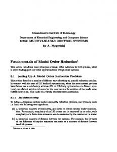
(Section 4.6), we will develop the point of view that any quantum state that has been in contact with a thermal reservoir is an algorithmically compressible object. This loophole helped us understand why—from an empirical point of view—simulation capabilities in quantum chemistry and condensed matter physics have been improving exponentially in recent decades [80, 149, 151]. The analysis and simulation methods that we will present in this article broadly define a geometric and quantum informatic program for sustaining this progress. 1.2.1. The geometry of reduced-order state-spaces This article’s mathematical methods are novel mainly in their focus upon the geometry of reduced-order quantum state-spaces. We will show that the quantum state-spaces that are most useful for large-scale simulation purposes generically have an algebraic structure that can be geometrically interpreted as a network of geodesic curves (rules) having nonpositive Gaussian curvature for all sections that contain a rule (Section 2). We will see that these curvature properties are essential to the efficiency and robustness of model order reduction. 1.2.2. The central role of covert measurements A technique that is central to our simulation recipes is to simulate all noise processes (including thermal baths) as equivalent covert measurement and control processes (Section 3). From a quantum informatic point of view, covert quantum measurement processes act to quench high-order quantum correlations that otherwise would be infeasibly costly to compute and store (Section 4). Thus the presence of noise can allow quantum simulations to evade the no-simulation arguments of Feynman [67]. 1.2.3. Background assumed by the presentation No reader will be expert in all of the disciplines that our analysis and simulation recipes embody, which are (chiefly) quantum mechanics in both its physical and informatic aspects, the engineering theory of model order reduction (MOR) and dynamical control, and the mathematical tools and theorems of algebraic and differential geometry. Indeed, the writing this article has made the authors acutely aware of their own considerable deficiencies in all of these areas. Recognizing this, we will describe all aspects of our recipes at a level that is intended to be broadly comprehensible to nonspecialists. 1.2.4. Overview of the analysis and simulation recipes We begin by surveying our chain of reasoning in its entirety. Figures 1–4 concisely summarize the simulation recipes and their geometric basis. In a nutshell, the recipes embody the orthodox quantum formalism of Fig. 1, as translated into the practical numerical algorithm of Fig. 2, which is based upon the algebraic structures of Fig. 3, whose functionality depends upon the fundamental geometric concepts of Fig. 4. The following overview summarizes those aspects of the simulation recipes that are fundamental, multidisciplinary, or novel, and it also seeks to describe the embedding of these recipes within the larger literature. 1.3. Overview of the formal simulation algorithm Formally, our simulation algorithms will be of the general quantum information-theoretic form that is summarized in Fig. 1. Steps A.1–2 of the algorithm are adopted, without essential change, from the axioms of Nielsen and Chaung [146], and our discussion will assume a background knowledge of quantum information theory at the levels of Chapters 2 and 8 of their text. Step A.3 of the simulation algorithm—projection of the quantum trajectory onto a statespace of reduced dimensionality—will be familiar to system engineers as projective model order reduction (as we will review in Sec. 1.4). We will also establish that projective MOR

1.3


8

Figure 1: Formal simulation by quantum model order reduction. Steps A.1–2 summarize the formal theory of the simulation of quantum systems (see, e.g., Nielsen and Chuang [146, chs. 2 and 8]). Step A.3 is a model order reduction of the Hilbert states |ψn i by projection onto a reduced-dimension Kähler manifold K (see e.g. Rewie´ nski [164]). Equivalently, Step A.3 may be viewed as a variety of Dirac-Frenkel variational projection (see, e.g., [133, 161]).

1.3


9

is formally identical to a method that is familiar to physicists and chemists as a variational order reduction of Dirac-Frenkel-McLachlan type [59, 76, 136] (see also the recent references [98, 133, 161]). For purposes of exposition, we define quantum model order reduction (QMOR) to be simply classical MOR extended to the complex state-space of quantum simulations. 1.3.1. The operational approach to quantum simulation Our simulation recipes will adopt a strictly operational approach to measurement and control, in the sense that we will require that the only information stream used for purposes of communication and control is the stream of binary stochastic outcomes of the measurement operations of Step A.2 of Fig. 1. Although it is not mathematically necessary, we will associate these binary outcomes with the classical “clicks” of physical measurement apparatuses, and we will develop a calibrated physical model of these clicks that will guide both our physical intuition and our simulation design. 1.3.2. The embrace of quantum orthodoxy Because the binary “clicks” of measurement outcomes are all that we seek to simulate, our analysis will regard the state trajectories {ψ 1 , ψ 2 , . . . , ψ n , . . . } as wholly inaccessible for all purposes associated with measurement and control, which is to say, as inaccessible for engineering purposes. We will analyze quantum state trajectories only with the goal of tuning the simulation algorithms to compress the trajectories onto low-dimension manifolds. In practice, this will mean that we mainly care about the geometric properties of quantum trajectories; this will be the organizing theme of our analysis. In the course of our analysis we will confirm—mainly to check our algebraic manipulations—that several of the traditional quantum measurement short-cuts that deal directly with wave-functions (e.g., uncertainty principles, wave function collapse, quantum Zeno effects) yield the same results as our “clicks-only” reductive formalism. But our simulations will not use these short-cuts, and in particular, we will never simulate quantum measurement processes in terms of von Neumann-style projection operators. The resulting simulation formalism is wholly operational, and can be informally described as “ultra-orthodox.” The operational approach will require some extra mathematical work—mainly in the area of stochastic analysis—but it will also yield some novel mathematical results, including a closed-form positive P -representation [153] of the thermal density matrix. We will derive this P -representation by methods that provably simulate finite-temperature baths. Thus the gain in practical simulation power will be worth the effort of the extra mathematical analysis. 1.3.3. The unitary invariance of quantum operations Our analysis will focus considerable attention upon the sole mathematical invariance of the simulation algorithm of Fig. 1, which is a unitary invariance associated in the choice of the quantum operations M in Step A.2. Our main mathematical discussion of this invariance will be in Section 3.2.1, our main discussion of its causal aspects will be in Section 3.3.6, our main review of the literature will be in Section 3.3.7, and it will be central to the discussion of all the simulations that we present in Section 4. We will see that the short answer to the question “What is this unitary invariance all about?” is that (1) it ensures that measured quantities respect physical causality, and (2) it allows quantum simulations to be tuned for improved efficiency and fidelity. In preparation, we caution readers that what we will call “quantum operations” are known by a great many other names too, including Kraus operators, decomposition operators and operation elements. These operations are discussed in textbooks by Nielsen and Chuang [146], Alicki and Lendi [6], Carmichael [40, 41], Percival [152], Breuer and Petruc-

1.3


10

cione [25], and Peres [155]. These texts build upon the earlier work of the mathematicians Stinespring [186] and Choi [48] and the physicists Kraus [122, 123], Davies [57], and Lindblad [131]. Shorter, reasonably self-contained discussions of open quantum systems can be found in articles by Peres and Terna [155], Adler [2], Rigo and Gisin [166], and Garcia-Mata et al. [83], and in on-line notes by Caves [46] and by Preskill [159]. It is prudent for students to browse among these works to find congenial points of view, because two of the above references are alike in the significance that they ascribe to the unitary invariance of quantum operations. This diversity arises because the invariance can be understood in multiple ways, including physically, algebraically, informatically, and geometrically. Our analysis will touch upon all these aspects, but much more than any of the above references, our approach will be geometric. 1.3.4. Naming and applying the Theorema Dilectum It is vexing that no short name for the unitary invariance associated with quantum operations has been generally adopted. For example, this theorem is indexed by Nielsen and Chuang under the unwieldy phrase “theorem: unitary freedom in the operator-sum representation” [146, thm. 8.2, sec. 8.2]. Because we require a short descriptive name, we will call this invariance the Theorema Dilectum, which means “the theorem of choosing, picking out, or selecting” (from the Latin deligo). As our discussions will demonstrate, this name is appropriate in both its literal sense and in its evocation of Gauss’ Theorema Egregium. In this article we will develop a geometric point of view in which the Theorema Dilectum is mainly a theorem about trajectories in state-space, and that the central practical role of the theorem in quantum simulations is to enable noisy quantum trajectories to be algorithmically compressed, such that efficient large-scale quantum simulation is feasible. To the best of our knowledge, no existing articles or textbooks have assigned to the Theorema Dilectum the central geometric role that this article focusses upon. The Theorema Dilectum is the first of two main technical terms that we will introduce in this review. To anticipate, the other is gabion, which is the name that we will give to state-space manifolds that support a certain kind of affine algebraic structure (see Figs. 3–4 and Section 1.5). When gabion manifolds are endowed with a Kähler metric, we will call the result a gabion-K¨ ahler manifold (GK manifold1 ). GK manifolds are the state-spaces onto which we will projectively compress the quantum trajectories of our simulations by exploiting the Theorema Dilectum. When we further impose an antisymmetry condition upon the state-space the result is a Grassmannian gabionK¨ ahler manifold (GGK manifold), and we will identify these manifolds as being both the well-known Slater determinants of quantum chemistry, and the equally well-known Grassmannian varieties of algebraic geometry. 1.3.5. Relation to geometric quantum mechanics Our recipes will embrace the strictly orthodox point of view that linear quantum mechanics is “the truth” to which our reducedorder K¨ ahlerian state-spaces are merely a useful low-order approximation. However, at several points our results will be relevant to a logically conjugate point of view, known as geometric quantum mechanics, which is described by Ashtekar and Schilling as follows [9] (see also [13, 172]): [In geometric quantum mechanics] the linear structure which is at the forefront in text-book treatments of quantum mechanics is, primarily, only a technical convenience 1 In a world in which every possible two-letter acronym is already in use, it is necessary to stipulate that this article’s definition of GK manifolds does not refer to the gyrokinetic (GK) simulation codes of plasma physics [65] nor to the generalized K¨ ahler (GK) manifolds of quantum field theory [8].

1.4

11

Overview of the numerical simulation algorithm

and the essential ingredients–the manifold of states, the symplectic structure and the Riemannian metric–do not share this linearity. Thus in geometric quantum mechanics, Kählerian geometry is regarded as a fundamental aspect of nature, while in our quantum MOR discussion, this same geometry is a matter of deliberate design, whose objective is optimizing simulation capability. Because our main focus is upon quantum MOR, we will comment only in passing upon those results that are relevant to geometric quantum mechanics (e.g., see the discussion in Section 2.12). 1.4. Overview of the numerical simulation algorithm The numerical simulation algorithm of Fig. 2 is simply the formal algorithm of Fig. 1 expressed in a form suitable for efficient computation. Note that Fig. 2 adopts the MATLABstyle engineering nomenclature of model order reduction, as contrasted with the physicsstyle bra-ket notation of Fig. 1. The algorithm of Fig. 2 is a fairly typical example of what engineers call model order reduction (MOR) [7, 81, 143, 147, 148]. Rewie´ nski’s thesis is particularly recommended as a review of modern nonlinear MOR ([164], see also [165]). 1.4.1. The main ideas of projective model order reduction We will now briefly summarize the main ideas of projective MOR in a form that well-adapted to quantum simulation purposes. We consider a generic MOR problem defined by the linear equation δψ = Gψ. Here ψ is a state vector, δψ is a state vector increment, and G is a (square) matrix. For the present it is not relevant whether ψ is real or complex. It commonly happens that ψ includes many degrees of freedom that are irrelevant to the practical interests that motivate a simulation. The central physical idea of MOR is to adopt a reduced order representation ψ(c), where c is a vector of model coordinates, having dim c dim ψ. The central mathematical problem of MOR is to describe the large-dimension increment δψ by a reduced-order increment δc. It is convenient to organize the partial derivatives of ψ(c) as a non-square matrix A(c) whose elements are [A(c)]ij ≡ ∂ψ i /∂cj . The reduced-order increment having least mean-square error is obtained by the following sequence of matrix manipulations: δψ = G ψ → A δc = G ψ → δc = AP G ψ → δc = (A† A)P (A† G ψ).

(1)

Here “P ” is the Moore-Penrose pseudo-inverse that is ubiquitous in data-fitting and model order reduction problems [160], “† ” is Hermitian conjugation, and the final step relies upon the pseudo-inverse identity XP = (X† X)P X† , which is exact for any matrix X [132]. This is the key step by which the master simulation equation is obtained that appears as Step B.3 at the bottom of Fig. 2. The great virtue of (1) for purposes of large-scale simulation is that (A† A) is a lowdimension matrix and (A† G ψ) is a low-dimension vector. Provided that both (A† A) and (A† G ψ) can be evaluated efficiently, and provided also that ψ(c) represents the “true” ψ with acceptable fidelity, substantial economies in simulation resources can be achieved. We will see that the required objectives of efficiency and fidelity both can be attained. 1.4.2. The natural emergence of K¨ ahlerian geometry The simulation equations, when expressed in covariant form (Step B.3 at the bottom of Fig. 2), provide a natural venue for asking fundamental geometric questions. ¯ For example, the low-dimension matrix ∂⊗∂κ ≡ 21 A† A is obviously Hermitian (whether ψ is real or complex). Of what manifold is it the Hermitian metric tensor? How does this manifold’s geometry influence the simulation’s efficiency, fidelity, and robustness?

1.4

Overview of the numerical simulation algorithm

12

Figure 2: Numerical algorithm for quantum model order reduction simulations. Steps B.1–3 are a numerical recipe that implements the simulation algorithm of Fig. 1. ¯ ¯ that are introduced in Step B.3 serve solely as variable The expressions (∂⊗∂κ) and (∂φ) names for the stored partial derivatives of the Kähler potential κ(¯ c, c) ≡ 12 hψ(¯ c)|ψ(c)i and 1 the dynamic potential φ(¯ c, c) ≡ 2 hψ(¯ c)|δG|ψ(c)i; it is evident that these partial derivatives wholly determine the simulation’s geometry and dynamics.

1.5

Overview of the unifying geometric ideas

13

To answer these questions, we will show that κ is the K¨ ahler potential of differential ¯ geometry, that the metric tensor ∂⊗∂κ determines the Riemannian curvature of our reduced order state-space, and that the choice of an appropriate curvature for this state-space is vital to the simulation’s efficiency, fidelity, and robustness. In preparing this article, our search of the literature did not find a previous analysis of MOR state-space geometry from this Riemannian/K¨ ahlerian point of view. We did, however, find recent work in communication theory by Cavalcante [42] and coworkers [43, 44] that adopts a similarly geometric point of view in the design of digital signal codes. Like us, these authors are unaware of previous similarly geometric work [43] “To the best of our knowledge this [geometric] approach was not considered previously in the context of designing signal sets for digital communication systems.” Like us, they recognize that “[These state-spaces] have rich algebraic structures and geometric properties so far not fully explored.” Also similar to us, they find [44] “The performance of a digital communication system depends on the sectional curvature of the manifold . . . the best performance is achieved when the sectional curvature is constant and negative.” Our analysis will reach similar conclusions regarding the desirable properties of nonpositive sectional curvature in the context of quantum MOR. Because the mathematical basis of this apparent convergence of geometric ideas between MOR theory and coding theory is not presently understood (by us at least), we will not comment further upon it. It is entirely possible that related work exists of which we are not aware. Model order reduction is ubiquitously practiced by essentially every discipline of mathematics, science, engineering, and business: the resulting literature is so vast, and the nomenclature so varied, that a comprehensive review is infeasible. It is fair to say, however, that the central role of Riemannian and Kählerian geometry in model order reduction is not widely appreciated. A major goal of our article, therefore, is to analyze the Riemannian/Kählerian aspects of MOR, and especially, to link the Kählerian geometry of quantum MOR to the fundamental quantum informatic invariance of the Theorema Dilectum. 1.4.3. Preparing for a K¨ ahlerian geometric analysis To prepare the way for our geometric ¯ analysis, at the bottom of Fig. 2 the pseudo-code defines storage variables named “(∂⊗∂κ)” ¯ and “(∂φ).” For coding purposes these names are of course purely conventional (an arbitrary string of characters would suffice), but these particular names are deliberately suggestive of partial derivatives of two scalar functions: κ and φ. To anticipate, κ will turn out to be the Kähler potential of complex differential geometry, which determines the differential geometry of the complex state-space, and φ will turn out to be a stochastic dynamical potential, which determines the drift and diffusion of quantum trajectories on the K¨ ahlerian state-space. The link between geometry and simulation efficiency thus arises naturally because both the geometry and the physics of our quantum trajectory simulations are determined by the same two scalar functions. 1.5. Overview of the unifying geometric ideas The main algebraic and geometric features of our state-space are summarized in Figs. 3–4. 1.5.1. The algebraic structure of the reduced-order state space The state-space of all our simulations will have the algebraic structure shown in Fig. 3. We will regard this algebraic structure as a geometric object that is embedded in a larger Hilbert space, and we will seek to understand its geometric properties, including especially its curvature, in relation to our central topic of quantum model order reduction.

1.5

14


|Ψi ≡

increasing order →

 n +j    2 +j   3 +j  c1 c1 c1 c +j 1 . . .  ..  ⊗  ..  ⊗  ..  ⊗ . . . ⊗  ...  n −j 3 −j 2 −j 1 −j c1 c1 c1 c1 1

increasing rank →

 n +j    2 +j   3 +j  c2 c2 c2 c +j 2 ..  ..   ..   ..    ⊗ ... ⊗ ⊗ ⊗ + . . . . n −j 3 −j 2 −j 1 −j c2 c2 c2 c2 1

+ ...  1 +j   2 +j   3 +j   n +j  cr cr cr cr ..   ..   ..  ..    + ⊗ ⊗ ⊗ ... ⊗ . . . . 1 −j 2 −j 3 −j n −j cr cr cr cr

≡

j X

tr A[1]i1 A[2]i2 . . . A[n]in |i1 , i2 , . . . , in i

i1 ,i2 ,...,in =−j

Figure 3: Algebraic definition of a gabion-Kähler (GK) state-space. The algebraic definition of a gabion-Kähler (GK) state-space (top) expressed equivalently as a matrix product state (MPS, bottom). By definition, the order of |ψi is the number of elements (spins) in each row’s outer product, the rank of |ψi is the number of rows. The matrices A[l]m that appear at bottom are, by definition, r × r matrices—hence rank r—having diagonal elements (A[l]m )kk ≡ lcm k and vanishing off-diagonal elements. Note that the matrix products are Abelian, such that the geometric properties of the state-space are invariant under permutation of the spins. Note also that when the above algebraic structure is antisymmetrized with respect to interchange of spins (equivalent to interchange of columns), the state becomes a sum of Slater determinants, or equivalently a join of Grasssmanian manifolds (a GGK manifold). In the language of algebraic geometry [53, 100], the geometric objects we will study are the algebraic manifolds that are associated with the projective algebraic varieties defined by the product-sums of Fig. 3. Although the literature on algebraic varieties is vast (and it includes many engineering applications [53]) and the literature on Riemannian sectional curvature is similarly vast, the intersection of these two subjects has apparently been little studied from an engineering point of view. This intersection, and especially its practical implications for quantum model order reduction, will be the main focus of our geometric investigations. The general algebraic structure of Fig. 3 is known by various names in various disciplines. As noted in the caption to Fig. 3, these structures are known to physicists as a matrix product states (often abbreviated MPS) which are widely used in condensed matter physics and ab initio quantum chemistry [55, 119, 156, 157, 173, 174, 191]; these references provide entry to a rapidly growing body of MPS-related literature.

1.5


15

Quantum chemists have known the algebraic structures of Fig. 3 as Hartree product states [102] since 1928. Upon antisymmetrizing the outer products, we obtain the Slater determinants [184] that are the fundamental building-blocks of modern quantum chemistry; upon summing Slater determinants, and (optionally) imposing linear constraints upon these sums, we obtain post-Hartree-Fock quantum states [54]. All of the theorems we derive will apply to Slater determinants and post-Hartree-Fock states as special cases (see Section 2.9). We will comment later in this section, too, upon the intimate relation of these ideas to density functional theory (DFT). Nuclear physicists embrace these same ideas under the name of wave function factorization [150]. Beylkin and Mohlenkamp [16] note that statisticians call essentially the same mathematical objects canonical decompositions and also parallel factors. As Leggett and co-authors have remarked with regard to the similarly immense literature on two-state quantum systems: “The topic of [this] paper is of course formally a problem in applied mathematics. . . . Ideas well known in one context have been discovered afresh in another, often in a language sufficiently different that it is not altogether trivial to make the connection. . . . [In such circumstances] the primary purposes of citations are to help the reader understand the paper, and the references in the text are chosen with this in mind” [129]. These same considerations will guide our discussion. The general utility of affine algebraic structures for modeling purposes first came to our attention in a highly readable Mathematical Intelligencer article by Mohlenkamp and Monzón [140]; two further articles by Beylkin and Mohlenkamp [15, 16] are particularly recommended also. Beylkin and Mohlenkamp call the algebraic structure of Fig. 3 a separated representation, and they have this to say about it [15]: When an algorithm in dimension one is extended to dimension d, in nearly every case its computational cost is taken to the power d. This fundamental difficulty is the single greatest impediment to solving many important problems and has been dubbed the curse of dimensionality. For numerical analysis in dimension d, we propose to use a representation for vectors and matrices that generalizes separation of variables while allowing controlled accuracy. . . . The contribution of this paper is twofold. First, we present a computational paradigm. With hindsight it is very natural, but this perspective was the most difficult part to achieve, and it has far-reaching consequences. Second, we start the development of a theory that demonstrates that separation ranks are low for many problems of interest. In a subsequent article Beylkin and Mohlenkamp go on to say [16] “The representation seems rather simple and familiar, but it actually has a surprisingly rich structure and is not well understood.” These remarks are remarkably similar in spirit to the coding theory observations of Cavalcante et al. that were reviewed in Section 1.4. For us, K¨ ahlerian algebraic geometry will provide a shared foundation for understanding the accelerating progress that all of the above large-scale computational disciplines have witnessed in recent decades. 1.5.2. The medieval idea of a gabion, and its mathematical parallels Deciding what to call the geometric state-space of quantum model order reduction is a vexing problem. We have seen that various plausible names include “Hartree products,” “Slater determinants,” “separated representations,” “matrix product states,” “wave function factorizations,” “productsum states,” “canonical decompositions,” and “parallel factors.” A shared disadvantage of the above names is that there is no precedent for associating them with the geometric properties that are the main focus of our investigations. We therefore seek an encompassing name for these state-spaces viewed as geometric entities.

1.5

16


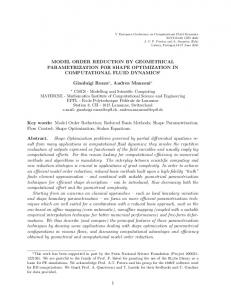
Finding no precedent in the literature, and desiring a short name having a long-established etymology, we will call them by the medieval name of gabions [192], or more formally, gabion manifolds (this name arose spontaneously in the course of a seminar). Most readers will have seen gabions numerous times, perhaps without recognizing that they have a well-established name. “Gabion” is the generic engineering name for a mesh basket that is filled with a weighty but irregularly-shaped material such as rocks or lumber, then stacked for purposes of reinforcement, erosion control, and fortification. In medieval times gabions were made of wicker or reed; Fig. 4(A) shows a typical medieval gabion. We will see that the defining geometry property of gabion manifolds is that they are possessed of a web of geodesic lines that constrain the curvature of the manifold, rather as the wicker reeds of a physical gabion constrain the curved rocks and boulders held inside. Like physical gabions, gabion manifolds come in a wide variety of sizes and shapes that are suitable for numerous practical purposes. We will postpone giving a formal—and necessarily rather abstract—mathematical definition of a gabion until Section 2.5. For the present our main objective is to informally describe the geometric properties that will motivate this formal definition. 1.5.3. The geometric properties of gabion-K¨ ahler (GK) manifolds The main geometric properties of GK manifolds that are relevant to quantum simulation are depicted in Fig. 4(BH). We will now survey these properties, and in doing so, we will introduce some of the nomenclature of K¨ ahlerian geometry. We begin our geometric overview by remarking that even though Hilbert space is a complex state-space, a common viewpoint among mathematicians is that a complex manifold is a real manifold that is endowed with an extra symmetry, called its complex structure (see Sections 2.2 and 2.6 for details). For purposes of our geometric analysis, we will simply ignore this complex structure until we are ready to apply the quantum Theorema Dilectum (Section 2.6). Until then we will treat gabion manifolds as real manifolds. In particular, the state-space of quantum mechanics has a natural real-valued measure of length. Specifically, along a time-dependent quantum trajectory |ψ(t)i it is natural to define a real-valued velocity v(t) whose formal expression can be written equivalently in several notations: dim H/2 X ˙ ˙ ˙ ˙ ˙ ¯ ˙ v(t) = g ψ(t), ψ(t) = hψ(t)|ψ(t)i = ψ(t) · ψ(t) = ψ¯˙ i (t)ψ˙ i (t) .

2

(2)

i=1

˙ ≡ ∂ψ(t)/∂t, and we have used first the abstract notation of differential geomeHere ψ(t) try (in which g(. . .) is a metric function), then the Dirac bra-ket notation of physics, then the matrix-vector notation of engineering and numerical computation, and finally the cumbersome but universal notation of components and sums over indices. We will assume an entry-level familiarity with all four notations, since this is a prerequisite for reading the literature. As a token of considerations to come, the factor of dim H/2 in the index limit of (2) above arises because we will regard a complex manifold like Cn as being a real manifold of dimension 2n. Thus we will regard the complex plane C as a two-dimensional (real) manifold, and an spin-1/2 quantum state as a point in a Hilbert space H having dim H = 4 (real) dimensions. This viewpoint leads to an ensemble of conventions that we will review in detail in Section 2.6. For now, we note that the arc length s along a trajectory is R s = v(t) dt, so that geometric lengths in quantum state-spaces are dimensionless. An equivalent differential definition is to assign a length increment ds to a state increment |dψi via (ds)2 = hdψ|dψi.

1.5

17


(a) medieval gabion

(b) ruled gabion geometry

(c) ruled geodesic basis

(d) geodesic completeness

(e) projective order reduction

(f) nonpositive curvature

n

(g) robust projective fidelity

(i) the Theorema Dilectum

ble

sta

ble

un

sta

too for dist sta ant bil ity

ble

sta

ble

sta

(h) the Theorema Egregium

Figure 4: Geometric principles of quantum model order reduction (QMOR). See Section 1.5 for a discussion of these principles.

1.5


18

Since we can now compute the real-valued length of an arbitrary curve on the gabion manifold, all of the usual techniques of differential geometry can be applied, without special regard for the fact that the state-space is complex. 1.5.4. GK manifolds are endowed with rule fields Beginning a pictoral summary of our geometric results, we first note that state-space gabions resemble physical gabions in that they are naturally endowed with a geometric mesh, which is comprised of a network of lines called rules, as depicted in Fig. 4(B). More formally, they are equipped with vector fields having certain mathematical properties (see (14) and Definition 2.1) such that the integral curves of the rule fields have the depicted properties. Postponing a more rigorous and general definition of gabion manifolds until later (see Section 2.5), we can informally define a gabion rule to be the quantum trajectory associated with the variation of a single coordinate n ckr in the algebraic structure of Fig. 3, holding all the other coordinates fixed to some arbitrary set of initial values. We see that gabion rules are rays (straight lines) in the embedding Hilbert space, and hence, the gabion rules are geodesics (shortest paths) on the gabion manifold itself. As depicted in Fig. 4(C), the set of all gabion points that belong to a rule is (trivially) the set of all gabion points itself, which is the defining characteristic of a gabion being ruled. Furthermore, we will show that at any given point, the vectors tangent to the rules that pass through that point are a basis set. 1.5.5. GK geometry has singularities Are gabion manifolds geometrically smooth, or do they have singularities? As depicted in Fig. 4(D), we will show that gabion manifolds have pinch-like geometric singularities. Algebraically these singularities appear whenever two or more rows of the product-sum in Fig. 3 are equal. Geometrically, we will show that the Riemann curvature diverges in the neighborhood of these singular points. However, it will turn out that the continuity of the geodesic rules is respected even at the singular points, so that gabion manifolds are geodesically complete. Pragmatically, this means that our numerical simulations will not become “stuck” at geometric singularities. 1.5.6. GK projection yields compressed representations As depicted in Fig. 4(E) model order reduction is achieved by the high-fidelity projection of an “exact” state |ψi in the large-dimension Hilbert space onto a nearby point |ψK i of the small-dimension gabion. It can be helpful to view this projection as a data-compression process. By analogy, the state |ψi is like an image in TIFF format; this format can store an arbitrary image with perfect fidelity, but consumes an inconveniently large amount of storage space. The projected state |ψK i on the gabion is like an image in JPEG format; lesser fidelity, but good enough for many practical purposes, and small enough for convenient storage and manipulation. We thus appreciate that data compression can be regarded as a kind of model order reduction; the two processes are fundamentally the same. 1.5.7. GK manifolds have negative sectional curvature Practical quantum simulations require that the computation of order-reducing projections be efficient and robust, just as we require image compression programs to be efficient and robust. As depicted in Fig. 4(F), order-reduction projection becomes ill-conditioned when the state-space manifold is “bumpy”, in which case a numerical search for a high-fidelity projection can become stuck at local minima that yield poor fidelity. We will prove that the presence of a ruled net guarantees that gabion manifolds are always smooth rather than bumpy. Resorting to slightly technical language to say exactly what we mean when we assert that gabion manifolds are not bumpy, in our Theorem 2.1 we will prove that a gabion has nonpositive sectional curvature for all sections on its geodesic net. This means that

1.5


19

gabion manifolds can be envisioned as a net of surfaces that have the special property of being saddle-shaped everywhere (as contrasted with generic surfaces having dome-shaped “bumps”). As depicted in Fig. 4(G), the saddle-shaped curvature helps ensure that orderreducing projection onto gabion manifolds is a numerically well-conditioned operation. 1.5.8. GK manifolds have an efflorescing global geometry As depicted in Fig. 4(H), when the number of state-space dimensions becomes very large, it becomes helpful to envision nonpositively curved manifolds as flower-shaped objects composed of a large number of locally Euclidean “petals.” This physical picture has been vividly conveyed by recent collaborative work between mathematicians and fabric artists [12]; the work of Taimina and Henderson on hyperbolic manifolds is particularly recommended [109]. When working in large-dimension spaces we will heed also Dantzig’s remark that “one’s intuition in higher dimensional space is not worth a damn!” [5]. For purposes of quantitative analysis we will rely upon Gauss’ Theorema Egregium [86] to analyze the Riemannian and Kählerian geometric properties of gabion manifolds. We will prove that “number of petals” becomes exponentially large, relative to dim K, such that the petals loosely fill the embedding Hilbert space. In this respect our geometric analysis will parallel the informatic analysis of Nielsen and Chuang [146]; their Fig. 4.18 is broadly equivalent to our Fig. 4(H). Our analysis will therefore establish two geometric properties of gabion manifolds: they are strongly curved, and they are richly endowed with straight-line rules. We will show that these gabion properties are essential to the efficiency, robustness, and fidelity of large-scale MOR. Later on, in Sections 4.6.4–4.6.6, we will establish a relation between these properties and compressive sampling (CS) theory. 1.5.9. GK basis vectors are over-complete We will nowhere assume that the basis vectors of the underlying algebraic structure of Fig. 3 are orthonormal; they might refer for example to the non-orthonormal gaussian basis states of quantum chemistry. A major geometric theme of our analysis, therefore, is that the negative sectional curvature of gabion manifolds helps generically account for the observed efficiency, fidelity, and robustness of gabion-based modeling techniques in many branches of science, engineering, and mathematics. 1.5.10. GK manifolds allow efficient algebraic computations Upon restricting our attention to the special case of gabion-K¨ ahler (GK) manifolds, we will show that the existence of a ruled geodesic net allows the sectional curvature and the Riemann curvature tensors of GK manifolds to be calculated easily and efficiently. To anticipate, we will present data from Riemann curvature tensors having dimension up to 188, which we believe are the largestdimension curvature tensors yet numerically computed. We will see that it is Kraus’ “long list of miracles” that makes large-scale numerical curvature computations feasible, and that these same miracles are equally essential to large-scale quantum dynamical calculations. 1.5.11. GK manifolds support the Theorema Dilectum One geometric idea remains that is key to our simulation recipes. For gabion manifolds to represent quantum trajectories with good fidelity, some physical mechanism must be invoked to compress quantum trajectories onto the petals of the gabion state-space. That key mechanism is, of course, the Theorema Dilectum that was mentioned in Section 1.3.4. From a geometric perspective, the Theorema Dilectum guarantees that noise can always be modeled as a measurement process that acts to compress trajectories onto the GK petals. As depicted in Fig. 4(I), quantum simulation can be envisioned geometrically as a process in which compression toward the GK petals, induced by measurement processes, competes with expansion away from the petals, induced by quantum dynamical processes. The balance of these two competing mechanisms determines the MOR dimensionality that is

1.5


20

required for good fidelity—the “petalthickness.” Algebraically this petal thickness increases in proportion to the rank of the product-sum algebraic structure of Fig. 3. Thus for us, trajectory compression is not a mathematical “trick,” but rather is a reasonably well-understood and well-validated quantum physical mechanism, originating in the Theorema Dilectum, that compresses quantum trajectories to within an exponentially small fraction of the Hilbert phase space. This noise-induced trajectory compression is the loophole by which QMOR simulations evade the no-simulation arguments of Feynman [67], as reviewed by Nielsen and Chuang [146, see their Section 4.7]. 1.5.12. GK manifolds support thermal equilibria We will see that this covert-measurement approach encompasses numerical searches for ground states. Specifically, by explicit construction, we will show that contact with a zero-temperature thermal reservoir can be modeled as an equivalent process of covert measurement and control, in which the role of “temperature” is played by the control gain, such that zero temperature is associated with optimal control. From this QMOR point of view, the calculation of a ground-state quantum wave function is a special kind of noisy quantum simulation, in which noise is present but masked by optimal control. This is how QMOR reconciles the strong arguments for the general infeasibility of ab initio condensed-matter calculations (as reviewed by, e.g., Kohn [121]) with the widespread experience that numerically computing the ground states of condensed matter systems is often, in practice, reasonably tractable [80]. 1.5.13. GK manifolds support fermionic states Readers familiar with ab initio quantum chemistry, and in particular with density functional theory (DFT) [28, 114, 121, see Cappele [39] for an introduction] will by now recognize that QMOR and DFT are conceptually parallel in numerous fundamental respects: the central role of the low-dimension Kähler manifold of QMOR parallels the central role of the low-dimension density functional of DFT; the closed-loop measurement and control processes of QMOR parallel the iterative calculation of the DFT ground state; QMOR’s fundamental limitation of being formally applicable only to noisy quantum systems parallels DFT’s fundamental limitation of being formally applicable only to ground states; QMOR and DFT share a favorable computational scaling with system size. Yet to the best of our knowledge—and surprisingly—the geometric techniques that that this article will deploy in service of QMOR have not yet been applied to DFT and related techniques of quantum chemistry and condensed matter physics [80]. A plausible starting point is to impose an antisymmetrizing Slater determinant-type structure upon the algebraic outer products of (3). Some analytic results that we have obtained regarding the Kählerian geometry of Slater determinants are summarized in Section 2.9. With further work along these lines, we believe that there are reasonable prospects of establishing a geometric/informatic interpretation, via the Theorema Egregium and the Theorema Dilectum, of the celebrated HohenbergKohn and Kohn-Sham Theorems of DFT [114] and their time-dependent generalization the Runge-Gross Theorem [28]. A physical motivation for this line of research is that the Theorema Dilectum of QMOR and the Hohenberg-Kohn Theorem of DFT embody essentially the same physical insight: the details of exponentially complicated details of quantum wave functions are only marginally relevant to the practical simulation of both noisy systems (QMOR) and systems near their ground-state (DFT). At present, the two formalisms differ mainly in their domain of application: QMOR is

1.6

Overview of contrasts between quantum and classical simulation

21

well-suited to simulating spatially localized systems at high temperature (e.g., spin systems) while DFT is particularly well-suited to simulating spatially delocalized systems (e.g., molecules and conduction bands) at low temperature. In the future, as QMOR is extended to delocalized systems while the methods of quantum chemistry are increasingly extended to dynamical systems [28, 80], opportunities will in our view arise for cross-fertilization of these two fields, both in terms of fundamental mathematics and in terms of practical applications. 1.6. Overview of contrasts between quantum and classical simulation In aggregate, the formal, numerical, algebraic, and geometric concepts summarized in the preceding sections and in Figs. 1–4 are in many respects strikingly parallel to similar concepts in the computational fluid dynamics (CFD), solid mechanics, combustion theory, and many other engineering disciplines that entail large-scale simulation using MOR. However, it is evident that quantum MOR is distinguished from real-valued (classical) MOR by at least four major differences, which we will now summarize. 1.6.1. The Theorema Dilectum is fundamental and universal The first difference is that the Theorema Dilectum describes an invariance of quantum dynamics that is fundamental and universal. Its physical meaning, as we will see, is that it enforces causality. Nonlinear classical system do not possess any similarly universal invariance, which is in our view a major contributing reason that “developing effective and efficient MOR strategies for nonlinear systems remains a challenging and relatively open problem” [164, p. 20]. Our results, both analytical and numerical, will suggest that noisy quantum systems are fundamentally no harder to simulate than nonlinear classical systems, provided that the Theorema Dilectum is exploited to allow high-fidelity dynamical projection of quantum trajectories onto a reduced-order state-space. 1.6.2. Quantum state-spaces are veiled The second difference is a consequence of the first. As discussed in Sec. 1.3, to fully exploit the power of the Theorema Dilectum we are required to embrace the ultra-orthodox principle of never looking at the quantum state space. Furthermore, when we examine classical state-spaces more closely, we find that they too are encumbered with ontological ambiguities that precisely mirror the “spooky mysteries” of quantum state-spaces. As discussed in Sections 3.2.7, this modern recognition of spooky mysteries in classical physics echoes work in the 1940s by Wheeler and Feynman [196, 197]. 1.6.3. Noise makes quantum simulation easier The third difference is that higher noise levels are beneficial to QMOR simulations, because they ensure stronger compression onto the GK petals, which allows lower-rank, faster-running GK state-spaces to be adopted. Later we will discuss the interesting question of whether this principle, together with the concomitant principle “never look directly at the quantum state-space,” have classical analogs. We will tentatively conclude that the Theorema Dilectum does have classical analogs, but that the power of this theorem is much greater in quantum simulations than in classical ones. 1.6.4. K¨ ahlerian manifolds are geometrically special Broadly speaking, Kählerian geometry is to Riemannian geometry what analytic functions are to ordinary functions. This additional structure is one of the reasons why the mathematician Shing-Tung Yau has expressed the view [200, p. 46] ”The most interesting geometric structure is the Kähler structure.” From this point of view, the geometry of real-valued MOR state-spaces is mathematically interesting, and the analytic extension of this geometry to Kählerian MOR state-spaces is even more interesting.

22

Let us state explicitly some of the analogies between analytic functions and Kähler manifolds. We recall that generically speaking, analytic functions have cuts and poles. These cuts and poles are of course exceedingly useful to scientists and engineers, since they can be intimately linked to physical properties of modeled systems. Similarly, the GK manifolds that concern us have singularities, as depicted in Fig. 4(D). Physically speaking, they are associated with regions of quantum state-space that locally are more nearly “classical” than the surrounding regions, in the sense that the local tangent vectors that generate highorder quantum correlations become degenerate. It is fair to say, however, that the deeper geometric significance of K¨ ahlerian MOR singularities remains to be elucidated. Just as contour integrals of analytic functions can be geometrically adjusted to make practical reckoning easier, we will see the Theorema Egregium allows the trajectories arising from the drift and diffusion of noise and measurement models to be geometrically (and informatically) adjusted to match state-space geometry, and thereby improve simulation fidelity, efficiency, and robustness. More broadly, Yau notes [200, p. 21]: “While we see great accomplishments for Kähler manifolds with positive curvature, very little is known for Kähler manifolds [having] strongly negative curvature.” It is precisely these negatively-curved Kähler manifolds that will concern us in this article, and we believe that their negative curvature is intimately linked to the presence of the singularities mentioned in the preceding paragraph. We hope that further mathematical research will help us understand these connections better.

2. The sectional curvature of gabion–K¨ ahler (GK) state-spaces We will now proceed with a detailed derivation and analysis of our quantum simulation recipes. Our analysis will “unwind” the preceding overview: first we analyze the geometry of Fig. 4, as embodying the algebraic structure of Fig. 3, using the numerical techniques of Fig. 2. Only at the very end will we calibrate our recipes in physical terms, via the quantum physics of Fig. 1. 2.1. Quantum MOR state-spaces viewed as manifolds To construct our initial example of a gabion state-space, we will consider the following algebraic function ψ(c), whose domain is a four-dimensional manifold of complex coordinates c = {c1 , c2 , c3 , c4 } and whose range in a four-dimensional Hilbert space is the set of points that can be algebraically represented as {c1 c3 , c1 c4 , c2 c3 , c2 c4 }. In the notation of Fig. 2 this function is  ψ1 − c1 c3 = 0   1 3  c c ψ2 − c1 c4 = 0 ψ(c) = 2 ⊗ 4 ⇔ , (3) c c ψ − c2 c3 = 0    3 ψ4 − c2 c4 = 0 where “⊗” is the outer product. The superscripts on the ci variables are indices rather than powers, as will be true throughout this section. From an algebraic geometry point of view, (3) defines a projective algebraic variety [53] (also called a homogeneous algebraic variety) over variables {ψi : i ∈ 1, 4} that is specified above in parametric form in terms of parameters {ci : i ∈ 1, 4}. By definition, our example of a gabion state-space manifold is the solution set of this algebraic variety, and thus our state space is an algebraic manifold. Physically speaking, ψ(c) is the most general (unnormalized) quantum state of two spin 1/2 particles sharing no quantum entanglement. We will now show that this state-space is a Kählerian manifold that has negative sectional curvature (under circumstances that we will describe) and that this property is ben-

2.2

23

Regarding gabion manifolds as real manifolds

eficial for simulation purposes (for reasons that we will describe). We begin by remarking that the basic algebraic construct “arg1 ⊗ arg2” that appears in (3) can be readily implemented by the built-in functions of most scientific programming languages and libraries; for example in MATLAB by the construct “reshape((arg1*arg2’)’,[],1)” and in Mathematica by the construct “Outer[Times,arg1,arg2]//Flatten”. Similar idioms exist for the efficient evaluation of more complex product-sum structures. Although we will not describe our computational codes in detail, they are implemented in MATLAB and Mathematica in accord with the general ideas and principles for efficient addition, inner products, and matrix-vector multiplication that are described by Beylkin and Mohlenkamp [16]. Practical computational considerations:

The abstract geometric point of view: From an abstract point of view, the algebraic structure

(3) can be regarded as a sequence of maps C

surjective

→

K

injective

→

(4)

H,

where C is the manifold of complex variables {c1, c2, c3, c4 }, the gabion manifold K is the range of ψ in H, and H is the larger Hilbert space within which K is embedded. To appreciate the surjective and injective nature of these maps, we notice in (3) that ψ(c) is invariant under {c1 , c2 , c3 , c4 } → {1, c2 /c1 , c1 c3 , c1 c4 }. More generally, it is clear that one coordinate can be set to any fixed nonzero value, without altering ψ(c), by an appropriate rescaling of the other three variables. In our example (3), the dimensions of the three manifolds C, K, and H are therefore dim C = 2 × 4 = 8,

dim K = 2 × 3 = 6,

dim H = 2 × 4 = 8,

(5)

where the factors of two arise because these are complex manifolds. We see that the map C → K is surjective (because dim K < dim C), while K → H is injective (because K is immersed in H).

2.1.1. Defining gabion pseudo-coordinates We will call the variables {c1 , c2 , c3 , c4 } pseudocoordinates. They are not ordinary coordinates because C → K is surjective rather than bijective, or to say it another way, open sets on C are not charts on K. Whenever we require an explicit coordinate basis, we can simply designate any one ck to be some arbitrary fixed (nonzero) value, and take the remaining {ci : i 6= k} to be coordinate functions. In practical numerical calculations—where these algebraic structures are called “separated representations,” “matrix product states,” or “Slater determinants”—pseudocoordinate representations are adopted almost universally. Therefore, we will sometimes simply call the c’s “coordinates”; this will make it easier to link the numerical algorithm of Fig. 2 to the geometric properties of K. 2.2. Regarding gabion manifolds as real manifolds Now we will begin analyzing in detail the curvature of the gabion manifold K. For geometric purposes it is convenient to regard H not as a complex vector space, but as a Euclidean space, such that ψ is a vector of real numbers that in our simple example has the eight components {ψ m } = { 0 otherwise.

(83)

(84)

Physically speaking, the smaller the variance ∆n (sop ), the smaller the quantum fluctuations in the expectation value hψn |sop |ψn i. We will now calculate the rate at which measurement operators act to minimize this variance. Considering an ensemble of simulation trajectories, we define the ensemble-averaged variance at the n-th simulation step to be E[∆n (sop )]. The algorithm of Fig. 1 evolves this mean variance according to " # m X X hψn |(Mjk )† sop Mjk |ψn i2 k † op 2 k op E[∆n+1 (s )] = E hψn |(Mj ) (s ) Mj |ψn i − (85) k )† M k |ψ i hψ |(M n n j j k=1 j∈{(+),(−)}

For compactness we write the increment of the variance as δ∆n (sop ) ≡ ∆n+1 (sop )]−∆n (sop ). Then for ergodic, synoptic, and bratrachian tunings the mean increment is  ergodic tuning,  0 op 2 2 op −4θ E[∆n (s )] synoptic tuning, E[δ∆n (s )] = (86)  −θ2 E[Fn (sop )] batrachian tuning. These results are obtained by substituting in (85) the spinometer tunings of (80–81), then expanding in θ to second order. Here F is the non-negative function 2 hψn |(sop )3 |ψn i − hψn |sop |ψn ihψn |(sop )2 |ψn i op Fn (s ) = . (87) hψn |(sop )2 |ψn i

Each term in the sequence {E[∆1 ], E[∆2 ], . . .} is nonnegative by (83), and yet for synoptic and batrachian tuning the successive terms in the sequence are non-increasing (because in (86) the quantities ∆2n (sop ) and Fn (sop ) are nonnegative and there is an overall minus sign acting on them); the sequence therefore has a limit. For synoptic tuning the limiting states are evidently such that ∆n (sop ) → 0, while for batrachian tunings Fn (sop ) → 0, which in both cases implies that the limiting states are eigenstates of sop . This proves Design Rule 3.7. Uniaxial spinometers with synoptic or batrachian tunings, but not ergodic tunings, asymptotically einselect eigenstates of the measurement generator. 3.4.4. Convergence bounds for the einselection of eigenstates We now prove a bound on the convergence rate of Design Rule 3.7. For QMOR purposes, this bound provides an important practical assurance that an ensemble of uniaxially observed spins never becomes trapped in a “dead zone” of state space. To prove the convergence bound, we notice that in the continuum limit θ 1 the increment (86) can be regarded as a differential equation in simulation time t ≡ n δt. For synoptic tuning the inequality E[∆2n (sop )] ≥ E[∆n (sop )]2 then allows us to derive—by integration of the continuum-limit equation—the power-law inequality E[∆n (sop )] ≤ E[∆0 (sop )]/(1 + 4nθ2 ).

(88)

3.4

Designs for spinometers

63

This implies that the large-n variance is O(n−1 ). This proof nowhere assumes that the initial ensemble is randomly chosen; therefore the above bound applies to all ensembles, even those whose initial quantum states are chosen to exhibit the slowest possible einselection. We conclude that for synoptic tuning the approach to the zero-variance limit is never pathologically slow. We have not been able to prove a similar bound for batrachian tuning, but numerical experiments suggest that both tunings require a time t ∼ δt/θ2 to achieve einselection. Proofs of stronger bounds would be valuable for the design of large-scale QMOR simulations. 3.4.5. Triaxial spinometers We now consider triaxial spinometers, in which three pairs of synoptic measurement operators (82) are applied, having as generators the spin operators {sx , sy , sz }, applied with couplings {θx , θy , θz }. 3.4.6. The Bloch equations for general triaxial spinometers In the general case we take θ1 6= θ2 6= θ3 . We define xn = {xn , yn , zn } = jhψn |s|ψn i to be the polarization vector at the n’th simulation step. This vector is normalized such that |xn | ≤ 1, with |xn | = 1 if and only if |ψn i is a coherent state. We further define δxn = xn − xn−1 . Taking as before E[. . .] to be an ensemble average over simulations, such that the density matrix of the ensemble is ρn = E[|ψn ihψn |], and therefore E[xn ] = j tr sρn , we readily calculate that the Bloch equation that describes the average polarization of the ensemble of simulations is 

   2  E[δxn ] E[xn−1 ] θy + θz2 0 0  E[δyn ]  = − 1    E[yn−1 ]  0 0 θx2 + θz2 2 2 2 E[δzn ] 0 0 θx + θ y E[zn−1 ]

(89)

Since it depends only linearly upon ρn , the above expression is invariant under the U transform of the Theorema Dilectum. We are free, therefore, to regard our spinometers as being ergodically tuned (80), such that the simulation can be equivalently regarded, not as three competing axial measurement processes, but as independent random rotations being applied along the x-axis, y-axis, and z-axis. The above Bloch equation therefore has the functional form that we expect upon purely classical grounds. 3.4.7. The einselection of coherent states Now we confine our attention to balanced triaxial spinometers, i.e., those having with θ1 = θ1 = θ1 ≡ θ, such that no one axis dominates the measurement process. Numerical simulations suggest that for synoptically tuned measurement processes, in the absence of entangling Hamiltonian interactions, simulated quantum trajectories swiftly converge to coherent state trajectories, regardless of the starting quantum state. We adopt Zurek’s (exceedingly useful) concept of einselection [201] to describe this process. We now prove that synoptic spinometric observation processes always induces einselection by calculating a rigorous lower bound upon the rate at which einselection occurs. Given an arbitrary state |ψi, we define a spin covariance matrix Λn to be the following 3 × 3 Hermitian matrix (of c-numbers): (Λn )kl ≡ hψn |sk sl |ψn i − hψn |sk |ψn ihψn |sl |ψn i.

(90)

This matrix covariance is a natural generalization of the scalar variance ∆n (sop ) (83), and in particular it satisfies a trace relation that is similar to (84) = j if |ψn i is a coherent spin state, tr Λn (91) > j otherwise.

3.4

64


ˆ, Here a coherent spin state is any spin-j state |ˆ xi, conventionally labeled by a unit vector x ˆ (see, e.g., Perelomov [153, eq. 4.3.35]). The algorithm of Fig. 1 such that hˆ x|s|ˆ xi = j x evolves the mean spin covariance according to " m X X (E[Λn+1 ])lm = E hψn |(Mjk )† sl sm Mjk |ψn i k=1 j∈{(+),(−)}

−

hψn |(Mjk )† sl Mjk |ψn ihψn |(Mjk )† sm Mjk |ψn i hψn |(Mjk )† Mjk |ψn i

#

(92)

For compactness we define the Λ-increment δΛn ≡ Λn+1 − Λn . Then by a series expansion of (92) similar to that which led from (85) to (86)—but with more indices—we find that for ergodic, synoptic, and batrachian tuning the mean increment is  ergodic tuning,  0 2 ? −4θ tr E[Λn ·Λn ] synoptic tuning, tr E[δΛn ] = (93)  (see text) batrachian tuning.

The “see text” for batrachian tuning indicates that we have found no closed-form expression simpler than several dozen terms; numerical experiments show that for this tuning the covariance exhibits random jump-type fluctuations that seemingly have no simple limiting behavior. In contrast, synoptic tuning’s increment has a strikingly simple analytic form, which was guessed as an ansatz and subsequently verified by machine algebra. Proceeding as in the proof of Theorem 1, and temporarily omitting the subscript n for compactness, we now prove that for Λ computed from |ψi by (90), the scalar quantity tr Λ·Λ? is non-negative for all |ψi, and vanishes if and only if |ψi is a coherent state. We remark ? that this proof is nontrivial because tr Λ·Λ by 0 is no means a positive-definite −1 0 quantity for +i ? general Hermitian Λ; an example is Λ = −i 0 , for which tr Λ·Λ = tr 0 −1 = −2. Because Λ is a Hermitian 3 × 3 matrix, it can be decomposed uniquely into a real ¯ and a real vector v = hψ|s|ψi/j by Λik = Λ ¯ ik +i/2 P3 ikl vl . Because symmetric matrix Λ l=1 the increment (93) is a scalar under rotations, without loss of generality we can choose a ˆ, z ˆ } such that {v·ˆ reference frame having basis vectors {ˆ x, y x, v·ˆ y , v·ˆ z } = {0, 0, z} and z ≥ 0. In this reference frame, the following decomposition is valid for any Hermitian matrix Λ ¯ an arbitrary symmetric matrix and z an arbitrary real number): (i.e., it holds for Λ tr Λ·(Λ? ) = j 2 (1 − z 2 )/2 + j 4 (1 − z 2 )2 /4

+ 2pa + 21 pb + 12 pc + 14 pd + 21 pe + jpf ,

(94)

where the residual terms pa , pb , . . . , pf are ¯2 + Λ ¯2 + Λ ¯2 , pa = Λ 12 13 23 ¯ 11 − Λ ¯ 22 )2 , pb = (Λ ¯ 33 )2 , pc = (Λ

¯ 33 )2 pd = (j 2 (1 − z 2 ) − 2Λ ¯ 11 + Λ ¯ 22 )2 − (j(j + 1) − (Λ ¯ 33 + j 2 z 2 ))2 pe = ( Λ 2 2 ¯ pf = j (1 − z ) − Λ33

(95)

We now prove that each term in this decomposition is non-negative. The terms pa , pb , pc , and pd are non-negative prima facie. The term pe vanishes for arbitrary |ψi in consequence ¯ 11 + Λ ¯ 22 + Λ ¯ 33 + j 2 z 2 = hψ|s2 + s2 + s2 |ψi = j(j + 1). That the of the spin operator identity Λ 1 2 3 remaining terms are non-negative in general follows from the spin operator inequalities −j ≤ hψ|s3 |ψi ≤ j and 0 ≤ hψ|s23 |ψi ≤ j 2 , which together with our reference-frame convention ¯ 33 < j 2 (1 − z 2 ). imply the inequalities −1 ≤ z ≤ 1 and Λ

3.4

65


Next, we show that the sum of terms (94) vanishes if and only if |ψi is coherent, i.e., if and only if |ψi = |ˆ z i. It is a straightforward exercise in spin operator algebra to show ¯ 33 = j 2 , Λ ¯ 11 = Λ ¯ 22 and that |ψi = |ˆ z i if and only if all of the following are true: z = 1, Λ ¯ ¯ ¯ Λ12 = Λ23 = Λ13 = 0; it follows that (94) vanishes if and only if |ψi = |ˆ z i. By reasoning similar to Theorem 1, we conclude: Design Rule 3.8. Triaxial spinometers with synoptic tunings asymptotically einselect coherent spin states. 3.4.8. Convergence bounds for the einselection of coherent states We now exploit the identity (94) to prove a bound on the convergence of Design Rule 3.8. Our strategy is similar to our previous proof of the bound for Design Rule 3.7. Substituting the identity j 2 (1 − z 2 ) = tr Λn − j in the first two terms of (94), and taking into account the nonnegativity of the remaining terms pa , pb , pc , pd , and pe , we obtain the following quadratic inequality in (tr Λn − j): tr Λn ·Λ?n ≥

1 2 (tr Λn

− j) + 41 (tr Λn − j)2 ≥ 0.

(96)

As an aside, our starting identity (94) was devised so as to imply a general inequality having the above quadratic functional form, in service of the proof that follows, but we have not been able to prove that the above coefficients { 12 , 14 } are the largest possible. Upon taking an ensemble average of the above inequality, followed by substitution in (93), followed by a continuum-limit integration, we obtain the following convergence bound for the ensemble-averaged trace covariance: tr E[Λn ] − j ≤

2(tr E[Λ0 ] − j) . (tr E[Λ0 ] − j)(exp(2nθ2 ) − 1) + 2 exp(2nθ2 )

(97)

It is instructive to restate this bound in terms of simulation time t = n δt. Taking the continuum limit Λn → Λ(t), noting that the timescale T1 = δt/θ2 is the conventional T1 that appears in the Bloch equations (89), defining for compactness of notation the initial trace covariance to be κ0 ≡ tr E[Λ(0)] − j, and assuming for the sake of discussion that κ0 1 (i.e, we assume that the initial ensemble is far-from-classical) the functional form of the above bound exhibits three asymptotic intervals, whose t-dependence is respectively O(1), O(1/t), and O(exp(−2t/T1 )):    κ0 (1 − κ0 t/T1 ) for 0 ≤ t/T1 . 1/κ0 , T1 /t for 1/κ0 . t/T1 . 1 (tr E[Λ(t)] − j) . (98)   2 exp(−2t/T1 ) for 1 . t/T1

The O(1) and O(1/t) behavior is functionally similar to the convergence bound established in (88) for the eigenvalue variance of Theorem 1, namely, an initial linear decrease, followed by an O(1/t) fall-off. Unique to triaxial spinometry (as far as the authors know) is the final exponentially rapid convergence to a coherent state. We note that convergence is complete within a time ∼ T1 that is independent of both the spin quantum number j and the overall dimensionality of the Hilbert space in which the spin is embedded. As with Theorem 1, this is a worst-case bound that applies to all ensembles, including (for example) exotic ensembles initialized with “Schröedinger’s cat” states. More particularly, it applies to large-dimensional ensembles in which each of n spins in a Hilbert space of overall dimension (2j + 1)n is synoptically observed.

3.4

66


3.4.9. Implications of einselection bounds for quantum simulations We now begin to have a quantitative appreciation of the geometric assertion of Fig. 4(i), that quantum simulations can be regarded as theaters in which the trajectory compression of synoptic observation opposes the creation of entanglement by Hamiltonian dynamics, with the balance between compression and expansion determining the dimensionality of the QMOR state space required for accurate simulation. Even stronger convergence bounds than those we have proved would be valuable in designing QMOR simulations. Especially useful would be more tunings in which noise is realized as an entangled measurement. Physically speaking, an entangled measurement is performed by interferometrically splitting a photon along n paths, scattering the photon from a different spin along each path, then recombining and measuring the photon by freely choosing among any of an exponentially large set of braidings and interferometric couplings of the downstream optical fibers. The analysis of such noise-equivalent tunings would require mathematical methods considerably more sophisticated than those we have deployed in this article. A known consequence of the Holevo-Schumacher-Westmoreland (HSW) theorem (which is the quantum analog of the Shannon channel capacity theorem) is that entangled measurements are necessary to maximize the information capacity of quantum channels [146, sec. 12.3.2]. If we hypothesize that quantum trajectory compression is in some sense proportional to information extracted by measurement, then the HSW theorem tells us that entangled measures will be more effective for QMOR purposes than the single-spin measures that we consider in this article. It is likely, therefore, that the search for more efficient QMOR techniques will benefit considerably from continued progress in quantum information theory. 3.4.10. Positive P -representations of the thermal density matrix Now we focus upon control and thermodynamics. For ˆt the thermal axis defined in (61), we modify the synoptic spinometer matrices such that √ ˆ k M(+) = e−iαθ(t×s)k [cos(θsk ) + sin(θsk )]/ 2 , (99) √ ˆ k M(−) = e+iαθ(t×s)k [cos(θsk ) − sin(θsk )]/ 2 , (100) where α is the control gain. We will call this a closed-loop triaxial spinometer with unitary feedback, because (as we will see) the unitary operators exp(±iαθ ˆt × s) act cumulatively to align the spin axis with ˆt. Closing the control loop does not alter the coherent einselection because the sole effect of a post hoc unitary operator on σ n is a spatial rotation. Since tr σ n ·σ ?n is a rotational scalar, (93) still holds. Thus we have Design Rule 3.9. Closed-loop triaxial spinometers with unitary feedback asymptotically einselect coherent states. The density matrix ρ of an ensemble of closed-loop triaxial spinometer simulations is described by sequence {ρ1 , ρ2 , . . .} whose increment is δρn =

3 X k=1

†k †k k k M(+) ρn M(+) + M(−) ρn M(−) − ρn ,

(101)

By a straightforward (but not short) calculation we find that δρn vanishes for ρn = ρth if and only if the closed-loop gain α satisfies α = − tanh 14 β

or

1/α = − tanh 14 β .

(102)

3.4

67


The following two trigonometric identities hold for either choice, and will be used in Section 4.1 to establish that the choice is immaterial in practical numerical simulations. 1/α + α = −2 coth 21 β

and

1/α − α = −2 csch 12 β

(103)

Defining as usual the dimensionless temperature T = 1/β, we see that an optimal control gain α → ±1 establishes a temperature T → ∓0, while a control gain |α| = 6 1 establishes a th finite temperature. We will establish later on that ρ solves δρn = 0 uniquely, because the Fokker-Planck equation for ρ has a unique stationary solution (thus the approach of the density matrix ρ to thermodynamic equilibrium never “stalls” or becomes trapped at false solutions). These results prove Design Rule 3.10. The density matrix of an ensemble of closed-loop triaxial spinometer simulations is asymptotically thermal. To connect (101) with the thermodynamic literature, we set ˆt = (0, 0, 1) and expand to order θ2 . The result is equivalent to a thermal model given by Perelomov (eq. 23.2.1 of [153]). Gardiner gives a similar model (eq. 10.4.2 of [84]). In Lindblad form we find δρn = − 21 γ(ν + 1) (s+ s− ρ − 2s− ρs+ + ρs+ s− ) − 12 γν (s− s+ ρ − 2s+ ρs− + ρs− s+ ) − θ2 (s3 s3 ρ − 2s3 ρs3 + s3 s3 ) , (104) √ √ where s+ = (s1 + is2 )/ 2 and s− = (s1 − is2 )/ 2 are raising and lowering operators, and we have adopted Perelomov’s variables γ = −4αθ2 and ν = −1/2 − (α + 1/α)/4.

3.4.11. The spin-1/2 thermal equilibrium Bloch equations The special case of spin-1/2 ˆ, particles in thermal equilibrium often arises in practice. Setting the polarization axis ˆt = z and allowing independent spinometric couplings {θx , θy , θz } as in (89), we find that the finite-temperature synoptic measurement operators (99) imply the following asymmetric Bloch equations (valid for j = 1/2 only):     E[δxn ] (α2 θx2 + θy2 + θz2 ) E[xn−1 ] 1    (105)  E[δyn ]  = −  (θx2 + α2 θy2 + θz2 ) E[yn−1 ]  2 1 2 2 2 E[δzn ] (1 + α )(θx + θy ) E[zn−1 ] + tanh 2 β

As expected on thermodynamic grounds, we see that the equilibrium polarization is E[z] = − tanh 12 β. These equations are a generalization of the usual Bloch equations, in the sense that the relaxation rates along the x-, y-, and z-axes can differ independently. We remark that for j > 1/2 the thermal Bloch equations do not have a closed analytic form; that is why this more general case is not considered here. 3.4.12. The spinometric Itˆ o and Fokker-Planck equations Now we focus on Itô and FokkerPlanck equations, aiming by our analysis to obtain both the already-validated positive P representation of Design Rule 3.2 and (in the large-j limit) both the linear Design Rules 3.3–5 and the fundamental quantum limits of Design Rule 3.6. We define a binary data three-vector dn = (d1n , d2n , d3n ) by k |ψ i , +1 for |ψn+1 i ∝ M(+) n k dn = (106) k −1 for |ψn+1 i ∝ M(−) |ψn i , Then {d1 , d2 , . . .} is a binary data record with calibration E[dn ] = gs E[xn ], where gs = 2θj

(107)

3.4

68


is the spinometer gain. We define a zero-mean stochastic variable W n by d n = gs x n + W n ,

(108)

such that (to leading order in θ) W n has the second-order stochastic properties of a discrete Wiener increment: E[(W n )k (W n0 )k0 ] = δnn0 δkk0 . (109) Then via an identity valid for |ψn i a coherent state, hψn |sk sl |ψn i = 12 jδkl + j(j − 12 )xk xj + 21 ij klm xm ,

(110)

the spinometer increments (99–b) are equivalent to an Itô increment δxn = xn+1 − xn = gs2 a(xn ) + gs b(xn )·W n .

(111)

For the drift vector a and diffusion matrix b we find a(x) = b(x) =

− 4j12 x [α(2j − 1)x·ˆt + (1 + 12 α2 )] + 4j12 ˆt [ α(2j + 1) − 12 α2 x·ˆt ] ,

1 2j [I

− x ⊗ x + α(ˆt ⊗ x − x·ˆt I)] .

(112a) (112b)

Design Rule 3.9, asserts that the Itô increment (111) confines the trajectory of xn to the unit sphere. The mean increment of the m’th radial moment |x|m must therefore vanish when |x| = 1. We check this by direct calculation, finding δEn [|x|m ] ∝ 21 m(m − 2)E[xn ·b(xn )·b† (xn )·xn ]

+ mE[|xn |2 (xn ·a(xn ) + 21 tr b(xn )·b† (xn ))] ,

(113)

which indeed vanishes for the a and b of (112a–b). By well-known methods [84], the Itˆ o increment (111) immediately yields a Fokker-Planck equation for the PDF pj (ˆ x). Setting ˆ ·ˆt we obtain the stationary state equation z=x ∂ [α(1 + z 2 ) + 2jα(1 − z 2 ) − z(1 + α2 )]pj (z) ∂z 1 ∂2 + [(1 − z 2 )(1 − 2αz + α2 )]pj (z) , 2 ∂z 2

0= −

(114)

which (when properly normalized) has a unique solution pj (ˆ x) = (α + 1/α − 2z)−2j−2 −1 × (2j + 1) (α + 1/α − 2)−2j−1 − (α + 1/α + 2)−2j−1 /π

(115) (116)

in which we see that the symmetry α → 1/α is indeed respected. Substituting α + 1/α = −2 coth 12 β per (103), and adjusting the normalization to match the P -representation convention (59) yields Design Rule 3.2.

3.4

69


3.4.13. The standard quantum limits to linear measurement To connect these results to Design Rules 3.2–3.6, we first write the Itô equation (111) in Langevin form by substituting R t+δt ˙ 0) δxn → t dt0 x(t (117) R t+δt 0 a(xn ) → r t dt a(x(t0 )) , (118) R t+δt 0 0 N 0 b(xn )·W n → rgs t dt b(x(t ))·x (t ) , (119)

where r = 1/δt is the rate at which increments occur, and xN (t) is white noise with crosscorrelation N 0 0 2 0 2 2 E[xN k (t)xk0 (t )] = δkk0 δ(t − t )/(rgs = δkk0 δ(t − t )/(4rj θ ) .

(120)

Then (111) becomes the integral of the Langevin equation

x˙ = rgs2 [a(x) + b(x)·(xM − x)] ,

(121a)

where xM (t) = x(t) + xN (t) is the measured spin axis. We see that x(t) is dynamically attracted toward the measured axis xM (t). Even openloop spinometers exhibit this attraction, since for α = 0 we find 1 1 ˙ α=0 = rgs2 [− 2 x + (I − x ⊗ x)·(xM − x)] . x| (121b) 4j 2j We remark that in uniaxial spinometry we saw that a similar einselection-by-attraction generates the “collapse” of |ψn i to an eigenstate, as described by Design Rule 3.7. This attraction is of course a fundamental tenet of the Hilbert ontology of Section 3.2.7. We now transform (121b) to the second-order Newtonian equation of an oscillator. To do this, we introduce a spring k and frequency ω0 by defining the operators q op = (~ω0 /jk)1/2 +s1 cos ω0 t − s2 sin ω0 t , (122a) op 1/2 p = (k~/jω0 ) −s1 sin ω0 t − s2 cos ω0 t . (122b) We confine our attention to those coherent states that have z ' −1, which with our sign conventions means systems having positive inverse temperature β, negative Hilbert feedback ˆ and polarization ˆt, such that x ˆ · ˆt ' −1. For gain α, and oppositely directed spin x op op these states the canonical commutator [q , p ] = −i~s3 /j ' i~ holds in the large-j limit. Defining the coherent oscillator coordinate q(t) to be q(t) = (j~ω0 /k)1/2 x(t) cos ω0 t − y(t) sin ω0 t , (123) we find that (121b) takes the linearized Newtonian form m¨ q = −k q + f n , q

m

(124a)

=q+q ,

(124b)

n

Here the spring k, mass m = k/ω02 , and coordinate q are to be understood in a generalized sense in which the system energy is 21 mq˙2 + 21 kq 2 . The measurement noise q n (t) is given from (123) in terms of the spinometer noises xN (t) and y N (t) of (120) by q n (t) = (j~ω0 /k)1/2 xN (t) cos ω0 t − y N (t) sin ω0 t , (125) and we find from (120) and (123) that the measurement noise q n (t) has a PSD Sqn of Sqn (ω)|ω'ω0 = ~ω0 /(4krjθ2 ) f n (t)

The force noise is then determined from (121b) to be the Hilbert transform and the Hilbert gain γ is found to be γ = 4krjθ2 /ω0

(126) f n (t)

=

γH[q n (t)],

where H is (127)

3.5

70

Summary of the design rules

3.4.14. Multiple expressions of the quantum noise limit It follows from the preceding results that the PSD of the spinometric force noise f n (t) can be expressed in multiple equivalent forms: expression Sf n (ω)|ω'ω0 = γ 2 Sqn (ω)|ω'ω0 = ~ / Sqn (ω)|ω'ω0 2

= ~γ = 4k~rjθ /ω0 2

physical interpretation force noise ∝ measurement noise

(128a)

force noise ∝ 1/(measurement noise)

(128b)

raw spinometer parameters

(128d)

force noise ∝ Hilbert backaction gain

(128c)

Each of the above relations has a plausible claim to expressing the “most natural” or “most fundamental” relation between measurement noise and force noise . . . despite the fact that no two physical interpretations are the same, and even though the interpretations given (128a) and (128b) seem contradictory. We further see by Design Rule 3.6 that these spinometric relations saturate the Hilbert noise limit (γSqn = ~), the Braginsky-Khalili limit (Sqn Sf n = ~2 ), and the Hefner-Haus-Caves limit (NF = 2); thus in some sense all of these fundamental quantum limits are embodied in the above family of spinometric relations. Acknowledging the self-consistency of this diversity, and appreciating its mathematical origin in the diversity of equivalent noise models that are supported by the Theorema Dilectum, helps us appreciate how the quantum noise literature can be so immensely large, and support so many different notations, physical arguments, and conclusions, and yet maintain its internal consistency. In a teaching environment, it is not practical to sustain a dispassionately anarchical equality among physical interpretations (128a-d). This article’s Hilbert ontology (Section 3.2.4) designates (128a) to be the fundamental relation, because it embodies the central Hilbert tenet that “measurement noise always back-acts upon system dynamics in such a way as to bring the state of the system into agreement with the measurement.” This choice is justified solely because it yields useful guiding principles for efficient quantum simulations. 3.5. Summary of the design rules In summary, we have established by Design Rules 3.7, 3.8 and 3.9 the quantum mechanism by which synoptic noise processes compress simulated quantum trajectories onto lowerdimension GK manifolds (as was promised in Section 1.5.11). We have established by Design Rule 3.10 that the effects of thermal reservoirs can be modeled as equivalent processes of covert measurement and control (as was promised in Section 1.5.12). And we have established by Design Rule 3.6 that the Hefner-Haus-Caves, Braginsky-Khalili, and Hilbert quantum noise limits are respected by QMOR simulations (as was promised in Section 3.2.6). The focus of the remainder of this article is to show, by explicit examples, that these design rules are sufficient to “enable the reader to proceed to the design and implementation of practical quantum simulations, guided by an appreciation of the geometric and informatic principles that are responsible for the overall simulation accuracy, robustness, and efficiency” (as was promised in the Introduction).

4. Examples of quantum simulation Now we turn our attention toward applying the preceding results in implementing practical quantum simulations.

4.1

Calibrating practical simulations

71

4.1. Calibrating practical simulations Our simulations provide data via the binary stream of defined in (106), which is low-pass filtered to produce a classical data record. We now work through, in detail, the process of computing and calibrating this data stream, and ensuring that it is numerically wellconditioned. We begin by considering the problem of determining, from physical system parameters, the measurement operation parameters {θ, α} in (99) and the clock rate r = 1/δt. In essence this calibration process requires that we invert systems of equations that include the Bloch equations (89) and (105), the Langevin equation (121b), and the mapping of spinometer parameters onto oscillator parameters (refeq: q definition). Whenever our simulations include a projective step, we must also ensure that the parameter of the projected Theorema Dilectum (54) satisfies 1. Physically speaking, imposing the small- condition ensures that the simulated trajectories evolve by drift and diffusion, rather than by “quantum jumps” that may be projectively ill-conditioned. Equally importantly, it ensures that they respect the informatic causality that is guaranteed by the Theorema Dilectum. 4.1.1. Calibrating the Bloch equations A common system to be simulated is a spin j = 12 in contact with a thermal reservoir. We desire that the three thermal relaxation rates along the x-, y-, and z- axes be {Γx , Γy , Γz } = {1/Tx , 1/Ty , 1/Tz } and that the equilibrium thermal density matrix be ρth ∝ exp(−βsz ), such that the equilibrium spin polarization p0 is − tanh 21 β as in (105). We thus have four physical parameters {Γx , Γy , Γz , β} with which to determine five raw spinometer parameters {θx , θy , θz , α, r}. Needing one more physical parameter, we note that the -parameters of the GK-projected Theorema Dilectum (54) is given for j = 1/2 spinometers from (105) by 2 = θ2 (1+α2 )/4, and so we impose as our fifth condition . 0.1 for all three spinometers (the cut-off 0.1 yielding in our experience well-converged numerical results). The equations below then follow from (101), (103), and (105): α = − tanh 14 β or −1/ tanh 41 β (freely chosen) 2x = Γz − sgn(1 − α2 )(Γx − Γy ) cosh 21 β /(4r) 2y = Γz + sgn(1 − α2 )(Γx − Γy ) cosh 12 β /(4r)

2z θi2

= [ Γx + Γy − Γz ] /(4r)

= 42i /(1 + α2 ) for i ∈ {x, y, z}

(129a) (129b) (129c) (129d) (129e)

Bloch-parameter calibration proceeds as follows. We first determine the spinometer gain α from (129a), and we will see that the choice “gain too big” versus “gain too small” is immaterial. The value of the spinometer click-rate r is then set from (129b-d) by requiring that min{x , y , z } . 0.1 for the reasons noted above. The values of the three spinometer phases {θx , θy , θz } are then determined from (129e). We remark upon three features. First, we see that insofar as simulation efficiency and numerical conditioning are concerned, the choice between the two options for the feedback gain α in (129a) is immaterial, since according to the above construction the spinometer click-rate r and the -parameters are unaffected. Second, for the special case Tz = T1 and Tx = Ty = T2 the above results reduce to the usual Bloch equations. Third, the positivity of the -parameters in (129b-d) requires that the Bloch relaxation rates satisfy the inequality (130) |Γx − Γy | cosh 21 β ≤ Γz ≤ Γx + Γy

4.1

72

Calibrating practical simulations

The authors suspect that the above Bloch inequality is tight, in the sense that no spin-1/2 Lindblad-form master equation can violate it, but we have not proved this. We remark that the above triaxially asymmetric Bloch equations and their associated relaxation rate inequality have (to the best of our knowledge) not appeared in the literature before. 4.1.2. Calibrating test-mass dynamics in practical simulations Now we consider test-masses (e.g., MRFM cantilevers) in contact with thermal reservoirs. Calibration proceeds by a line of reasoning similar to the above. We take the test-mass to be described by two physical parameters: the (dimensionless) temperature β = ~ω0 /(kB T ) and the (dimensionless) quality Q of the ring-down wave-form q(t) ∝ cos(ω0 t) exp(ω0 t/(2Q)). The four spinometer parameters to be determined are {j, θ, α, r}. The spin number j we take to satisfy j 1, and we will find that the precise value chosen for j is immaterial. For coherent states with z ' −1 as discussed in Section 3.4.12, the -parameter is found to be ' jθ2 (1 + α2 ). Calibration proceeds as follows: α = − tanh 41 β

or

−1/ tanh 41 β

2 = ω0 /(2Qr) coth 12 β jθ = /(1 + α ) 2

2

2

(freely chosen)

(131a) (131b) (131c)

We first determine the spinometer gain α from (131a). The value of the spinometer clickrate r is then set from (131b) by requiring that . 0.1 as in the Bloch equation case, and the spinometer phase θ is determined from (131c). We remark again that insofar as simulation efficiency is concerned, the choice between the two options for the feedback gain α in (131a) is immaterial, since the spinometer click-rate r is unaffected. We see also that for fixed quality Q, the simulation rate r is O(coth 12 β), which physically means that hot cantilevers are computationally more expensive to simulate than cold ones, as is reasonable. 4.1.3. Calibrating purely observation processes It can happen that we wish to directly observe a spin-1/2 particle along a single axis, nominally the z-axis, in an observation process in which the measured z-axis polarization z m (t) = z(t) + z n (t) has a specified (onesided) noise PSD Sz n . No thermodynamical feedback is applied. Then by reasoning similar to the preceding cases, we find from (120) that the calibration relations are 2 = 1/(2rSz n )

(132a)

θ = 4

(132b)

2

2

and as before, the spinometer click rate r is determined by requiring . 0.1. Similarly, if we wish to simulate the continuous observation of a test-mass coordinate q(t), with no thermodynamical feedback, the required calibration equations are given from (120) and (123) in terms of the measurement noise PSD Sqn by 2 = ~ω0 /(4rkSqn ) jθ = 2

2

(133a) (133b)

where again the spinometer click rate r is determined by requiring . 0.1. We remark that in all of the above cases the raw binary data stream (106) of the simulation must be low-pass filtered in order to obtain a (noisy) data record that will have the above statistical properties within the filter passband having. This filtering closely models the way that real experimental signals (for example, a continuously measured cantilever motion) are displayed upon oscilloscopes.

4.2

Three single-spin MRFM simulations

73

Figure 10: Simulation of single electron moment detection by MRFM. 4.2. Three single-spin MRFM simulations With reference to Fig. 10, we now turn our attention to the simulation of the IBM singlespin MRFM experiment [170] . We will initially present the simplest possible class of simulations that reproduce the data of that experiment, postponing a discussion of more detailed simulations until Section 4.4. Our goal is to illuminate the central role of the Theorema Dilectum in answering the question that was raised in Section 1.1: “How does the Stern-Gerlach experiment work?” All three columns of Fig. 10 show a simulated thirteen-hour experiment (the length of the IBM experiment). The time-spacing δt = 1/r between spinometric clicks is set to 7.1 ms; thus approximately 6.6 × 106 time-steps were simulated. In each column, the experimental data are simulated as arising from three competing spinometric processes. Spin relaxation was simulated by x-axis and y-axis spinometers having θx = θy = 0.093. The consequent spin relaxation time from (105) is Tz = 2/ r(θx2 + θy2 ) ' 0.76 s as was observed in the IBM experiment. Measurement effects were simulated by a z-axis spinometer having θz = 0.026, and the consequent measurement noise PSD from (120) is Sz n = 2/(rθz2 ), which numerically corresponds to a noise level of 11.5 Bohr magnetons of noise in one root-Hertz of bandwidth, as was observed in the IBM experiment. For visualization purposes only, all time-domain data streams shown in Fig. 10 were low-pass filtered with a time constant τ = Tz = 0.76 s. The following discussion is insensitive to the above experimental details, and applies to

4.2

Three single-spin MRFM simulations

74

all experiments of Stern-Gerlach type in which the signal-to-noise ratio (SNR) is low, such that continuous monitoring over extended periods of time is required to observe the effect. In the next three sections, we simulate the spin relaxation of the IBM single-spin MRFM experiment by three different unravelings: batrachian, ergodic, and synoptic. We will see that the three unravelings lead to three very different classes of quantum trajectories, and hence, three very different answers to the question “How does the Stern-Gerlach experiment work?” Nonetheless, as guaranteed by the Theorema Dilectum, we will find that the simulated experimental data are identical for all three unravelings. We now work through the mathematical and physical details of how this comes about. 4.2.1. A batrachian single-spin unraveling The left-hand column of Fig. 10 shows a simulation in which thermal noise is unravelled as a batrachian process, whose measurement operations are given algebraically in (81) and which are depicted in hardware-equivalent form in Figure 9(b). This is by far the easiest simulation to analyze in closed form: the spin polarization jumps randomly between ±1, driven by the batrachian jumps of the thermal reservoir, while being continuously measured by the (noisy) cantilever. The simulated data stream is therefore a random telegraph signal with added white noise, such that the mean-square quantum spin polarization inferred from the data is unity. We conclude that from the batrachian point of view, the Stern-Gerlach effect (meaning, that the mean-square spin polarization is measured to be unity) comes about because noise is a quantized jump process, such that the mean-square spin polarization always is unity. 4.2.2. An ergodic single-spin unravelling The middle column of Fig. 10(b) shows a simulation in which thermal noise is unravelled as an ergodic process, whose measurement operations are given algebraically in (80) and which are physically depicted in Figure 9(a). Physically speaking, the spin polarization is driven by random magnetic fields, such that the mean-square quantum polarization is 1/3. Now a subtle effect comes into play. The z-axis measurement process back-acts upon the spin state, such that whenever an “up” fluctuation in the data is observed, the spin state is “dragged” toward a positive polarization. This effect is evident in the simulated data. The consequence of state-dragging back-action is that the measured mean-square polarization is larger than the mean-square polarization of the underlying quantum state. It would be quite a complicated task to calculate the resulting data statistics from (e.g.) the appropriate Itˆ o, Langevin, and Fokker-Planck equations. Fortunately, the Theorema Dilectum does this mathematical work for us: the data statistics are guaranteed to be exactly the same random telegraph statistics as in the Batrachian case. We conclude that from the ergodic point of view, the Stern-Gerlach effect (meaning, that the mean-square spin polarization is measured to be unity) comes about because measurement is a Hilbert process (meaning, it accords with the state-dragging Hilbert back-action ontology of Section 3.2.4). 4.2.3. A synoptic single-spin unravelling The right-hand column of Fig. 10(c) shows a simulation in which thermal noise is unravelled as an synoptic process, whose measurement operations are given algebraically in (82) and which are physically depicted in Figure 9(c). In synoptic unravelling, all processes are measurement processes, and each process seeks to align the spin polarization along its own axis. In our simulation, the x-axis and y-axis measurement processes are considerably stronger than the z-axis process. In consequence of the Hilbert state-dragging effect, the spin polarization now points predominantly in the equatorial direction, such that the mean-square quantum polarization is only ∼ 0.05. Again it would be quite a complicated task to calculate the resulting data statistic from Itô equations, etc., and again the Theorema Dilectum does this mathematical work for us:

4.3

So how does the Stern-Gerlach effect really work?

75

as in the preceding two cases, the data statistics are random telegraph statistics with added white noise. We conclude that from the synoptic point of view, the Stern-Gerlach effect is not associated with “wave function collapse,” but rather comes about (as in the ergodic case) because measurement is a Hilbert process. 4.3. So how does the Stern-Gerlach effect really work? We are now in a position to answer more completely the question “How does the SternGerlach effect really work?” We answer as follows: “Nothing definite can be said about the internal state of noisy systems, either at the classical or at the quantum level. It is best to pick an ontology that facilitates rapid calculations and suggests interesting mathematics. For purposes of large-scale quantum simulation, a particularly useful ontology is one in which all noise processes are conceived as equivalent covert measurement processes. In this ontology, the Stern-Gerlach effect works because competing measurement processes exert a Hilbert back-action mechanism that ‘drags’ quantum states into agreement with measurement. In consequence of these competing Hilbert measurements, experimental data having the statistics of random telegraph signals are obtained even when no quantum jumps are present.” Of course, we saw in the three simulations of Fig. 10a–c that other explanations are perfectly reasonable, and that is why in Section 1.1.1 we embraced Peter Shor’s maxim: “Interpretations of quantum mechanics, unlike Gods, are not jealous, and thus it is safe to believe in more than one at the same time,” to which we now append the caveat “provided that all interpretations respect the fundamental mathematical and physical invariance of the Theorema Dilectum.” 4.4. Was the IBM cantilever a macroscopic quantum object? The least realistic element of the proceeding simulations is the modeling of the cantilever as a single z-axis spinometer having quantum number j = 1/2. A more realistic model would have treated the cantilever as a large-j quantum object subject both to thermal noise processes and to experimental measurement processes. However, we can appeal to the Theorema Dilectum to show that these refinements would not change the simulated data at all. The reason is that both the cantilever thermal reservoir and the experimental (interferometric) cantilever measurement process can be modeled as synoptic processes that compress the cantilever’s quantum state to a coherent state. Then modeling the spin relaxation as a batrachian process, the output of the resulting (effectively semi-classical) batrachian simulation will be precisely the random telegraph signal that was obtained in the simpler batrachian simulation of Section 4.2.1 above. It follows by the Theorema Dilectum that all quantum simulations of the cantilever, even elaborate large-j simulations in which a non-coherent quantum cantilever state is entangled with the quantum spin state, will simulate the same random telegraph data statistics as the simpler simulations already given, and in particular, will yield an observed mean-square polarization of unity. This leads to an interesting question: what was the “real” quantum state of the IBM cantilever? We have seen that this question has a well-posed answer only insofar as there is agreement upon the “real” noise and observation processes acting upon the cantilever, such that the tuning ambiguity of the Theorema Dilectum does not come into play. If we stipulate that the “real” cantilever thermal noise and the “real” spin relaxation are due to ergodic physical processes, then the IBM experiment can only be “really” described in terms of a spin-state that is quantum-entangled with the cantilever state, in which the observed mean-square polarization of unity is “really” due to the state-dragging Hilbert

4.5

The fidelity of projective QMOR in spin-dust simulations

76

back-action associated with the cantilever measurement process. In other words, the IBM experiment “really” observed the cantilever to be a macroscopic quantum object. As quantum objects go, the IBM cantilever was exceptionally large [170]: its resonant frequency was ω0 /(2π) = 5.5 kHz, its spring constant was k = 0.011 mN/m, and its motional mass was m = k/ω02 = 9.1 pg. The preceding paragraphs are an argument for regarding this cantilever to be among the stiffest, slowest, most massive dynamical systems whose quantum nature has been experimentally confirmed. Such measurements are significant from a fundamental physics point of view, in probing the limits of quantum descriptions of macroscopic objects, as reviewed by Leggett [125, 126, 127, 128]. Any line of reasoning that is as brief as the preceding one, about a subject that is as subtle as macroscopic quantum mechanics, is sure to have loopholes in it. A major loophole is our modeling of decoherent noise as a Markovian process. As reviewed by Leggett et al. [129], spin decoherence in real experiments is (of course) due to non-Markovian quantumentangling interactions. We now turn our attention to the algorithmic and numerical challenges of simulating such systems. 4.5. The fidelity of projective QMOR in spin-dust simulations As test cases, we computed what we will call spin-dust simulations. Spin-dusts are quantum systems that are deliberately constructed so as to have no symmetries or spatial ordering. Their sole purpose is to provide a well-defined test-bed for numerical and analytic studies of the fidelity of projective quantum model order reduction. Spin-dusts couple pairs of spin-1/2 particles {j, k} via a dipole-dipole interaction Hamiltonian Hjk that is given by ( sj · [I − 3njk ⊗ njk ] · sk for j 6= k Hjk = (134) sj · njk for j = k The unit vectors njk are chosen randomly and independently for each {j, k}, and we note that self-coupling is allowed. Physically we can think of spin-dusts as broadly analogous to—but less structured than—systems such as the interacting spins in a protein molecule. In our simulations each spin is randomly coupled to four other spins, in addition to its self-interaction. Then it is easy to show that tr H = 0 and tr H 2 / dim H = nspin , which is to say, the per-spin energy of our spin-dusts has zero mean and unit variance. The time-scale of the spin dynamics of the system is therefore unity. We further stipulate that each spin is subject to a triaxial spinometric observation process having relaxation time Tx = Ty = Tz = 10. Thus the time-scale of decoherent observation is ten-fold longer than the dynamical time-scale. Simulations were computed with a time-step δt = 0.1 and spinometric couplings θx = θy = θz = 0.1, using the sparse matrix routines of Mathematica. The numerical result was an “exact” (meaning, full Hilbert space) quantum trajectory |ψ0 (t)i. These trajectories were then projected on GK manifolds of various order and rank by the numerical methods of Section 2.12. The main focus of our numerical investigations was the fidelity of the projected states |ψK (t)i relative to the exact states |ψ0 (t)i.

4.5.1. The fidelity of quantum state projection onto GK manifolds With reference to Fig. 11(a), simulations were conducted with numbers of spins n ∈ 1, 18, having random dipole coupling links as depicted. The median quantum fidelity was then computed, as a function of n, for GK rank r ∈ {1, 2, 5, 10, 20, 30} (see Fig. 3 for the definition of GK rank). Both synoptic and ergodic unravelings were simulated. Typically |ψ0 i(t) was projected at thirty different time-points along each simulated trajectory, always at times t > 100 to ensure that memory

77


(a) Dipole-dipole interactions of four-neighbor spin dust order = 2 (2 spins)

order = 3

order = 4

dipole coupling spin

spin

order = 5

order = 6

order = 7

(b) Quantum fidelity of state-space projection for synoptic and ergodic noise unraveling quantum fidelity

4.5

1 synoptic noise unraveling ergodic noise unraveling

order = 8

order = 9

order = 10

order = 11

order = 12

order = 13

quantum fidelity

0.3

order = 17

order = 18

order = 16

• no spatial symmetry • no spatial ordering • random coupling • dim H = 2 order

quantum fidelity

order = 15

rank = 2

1

0.3 order = 14

state-space rank = 1

rank = 5

rank = 10

1

0.3

rank = 20

rank = 30

2 4 6 8 10 12 14 16 18 order (number of spins)

2 4 6 8 10 12 14 16 18 order (number of spins)

Figure 11: The dependence of QMOR fidelity upon GK order and rank. of the (randomly chosen) initial state was lost. We remark that numbers of spins n > 18 could not feasibly be simulated on our modest computer (an Apple G5). The quantum fidelity of a projected state |ψK i was defined to be [146, Section 9.2.2] 1/2 f = |hψK |ψ0 i|/ hψK |ψK ihψ0 |ψ0 i .

(135)

As shown in Fig. 11(b), for ergodic unravellings large-n quantum fidelity fell-off exponentially, while for synoptic unravelings large-n fidelity remained high. No mathematical explanation for the observed exponential fall-off in ergodic unravelling fidelity is known. The asymptotic large-n behavior of the synoptic fidelity also is unknown. In particular, for systems of hundreds or thousands os spins, would the empirical rule-ofthumb “GK rank fifty yields high fidelity for spin-dust systems” still hold true? These are important topics for further investigation. The achieved high-fidelity algorithmic compression was large: an 18-spin exact quantum state |ψ0 (t)i is described by 218 independent complex numbers, while an order-18 rank 30 GK state |ψK (t)i—as seen at lower right in Fig. 11(b)—is described by 30 × (18 + 1) = 570 independent complex variables. The dimensional reduction is therefore 460-to-1. 4.5.2. The fidelity of spin polarization in projective QMOR We next turned our attention to measures of local quantum fidelity, as depicted in Fig. 12. All simulated trajectories in this figure were for n = 15 spin-dust. The first such measure we consider are the direction

4.5

direction cosine

1.0

rank = 1

rank = 5

rank = 10

rank = 20

rank = 50

0.0

-1.0

Wootters’ quantum concurrence

quantum operator covariance

0.2

mutual quantum information

measured on the projected Kähler space

78


0.0

-0.2

0.2

0.0

-0.2 1.0

single spins linked pairs

0.5

non-linked pairs

0.0

measured on the full Hilbert space Figure 12: Measures of projective fidelity for n = 15 spin-dust. ˆ cosines hψ|s · m|ψi/j for randomly spins, randomly chosen trajectory points, and randomly ˆ chosen unit vectors m. One hundred randomly chosen data points are shown. We observe that the rank-one GK manifold does an excellent job of representing the spin direction cosines, which can be regarded as (essentially) classical quantities. 4.5.3. The fidelity of operator covariance in projective QMOR As a measure of pair-wise quantum correlation, we examined the spin operator covariance. With reference to (90), this quantity is given by Σjk = 4Λkl = hψ|σj σk |ψi − hψ|σj |ψihψ|σk |ψi.

(136)

which vanishes for rank-1 (product states). The second row of Fig. 12 plots Σkl for one hundred randomly chosen trajectory points, and randomly chosen spins, having randomly chosen indices j and k. We observe that GK ranks in the range 20–50 are necessary for projection to preserve pair-wise quantum correlation with good accuracy. 4.5.4. The fidelity of quantum concurrence in projective QMOR As a measure of pairwise quantum entanglement, we examined Wooters’ quantum concurrence [199]. The concur-

4.6

Quantum state reconstruction from sparse random projections

79

rence is computed as follows. Let ρAB be the reduced density matrix associated with spins A and B. Let λi be eigenvalues of the non-Hermitian matrix ρAB ρÃB , in decreasing order, where ρÃB = (σy ⊗ σy )ρ?AB (σy ⊗ σy ). Then the concurrence c is defined to be p p p p c = λ1 − λ2 − λ3 − λ4 (137)

It can be shown that the concurrence vanishes for product states, and that spins are pairwise entangled if and only if c > 0. In the third row of Fig. 12, we observe that coupled spin-pairs are far more likely to be quantum-entangled than non-coupled spin-pairs, as expected on physical grounds. We further observe that GK ranks in the range 20–50 are necessary for projection to preserve concurrence with good accuracy. 4.5.5. The fidelity of mutual information in projective QMOR As a measure of pair-wise quantum information, we examined von Neumann’s mutual information [146, Section 11.3], which is computed as follows. For a general density matrix ρ we define the von Neummann entropy S(ρ) = − tr ρ log2 ρ. Then for spins A and B the mutual information is given by S(ρA ) + S(ρB ) − S(ρAB )

(138)

It is known that the mutual information vanishes for product states, and that this quantity is otherwise positive in general. In the fourth row of Fig. 12, we observe that coupled spin-pairs share more mutual quantum information than non-coupled pairs, as expected on physical grounds. We further observe that GK ranks in the range 20–50 are necessary for projection to preserve mutual quantum information with good accuracy. As a quantitative summary of this observation, the 15-spin simulations of Fig. 12 predict 15 single-spin density matrices ρA and 105 pairwise reduced density matrices ρAB (in addition to higher-order correlations). Each of the single-spin density matrices has 3 (real) degrees of freedom, and each pairwise density matrix introduces 9 more (real) independent degrees of freedom, for a total of 990 independent degrees of freedom associated with the one-spin and two-spin reduced density matrices. In comparison, the rank-50 GK manifold onto which the quantum states are projected is described by Kählerian coordinates having (it can be shown) 1600 locally independent coordinates. Using 1600 state-space coordinates to encode 990 physical degrees of freedom represents a level of MOR fidelity that (obviously) cannot be improved by more than another factor of two or so. The mathematical origin of this empirical algorithmic efficiency is not known. 4.6. Quantum state reconstruction from sparse random projections We will conclude our survey of spin-dust simulations with some concrete calculations that are motivated by recent advances in the theory of compressive sampling (CS) and sparse reconstruction. It will become apparent that synoptic simulations of quantum trajectories mesh very naturally with CS methods and ideas. To the best of our knowledge, this is the first description of CS methods applied to quantum state-spaces. Our analysis will mainly draw upon the ideas and methods of Donoho [61] and of Candès and Tao [37], and our discussion will assume a basic familiarity with these and similar CS articles [30, 31, 32, 34, 36], especially a recent series of articles and commentaries on the Dantzig selector [17, 29, 38, 64, 79, 137, 167]. Our analysis can alternatively be viewed as an extension to the quantum domain of the approach of Baraniuk, Hegde, and Wakin [11, 47, 194] to manifold learning [188] from sparse random projections. Our objectives in this section are:

4.6


80

• establish that synoptically simulated wave functions ψ 0 are compressible objects in the sense of Candès and Tao [37], • establish that high-fidelity quantum state reconstruction from sparse random projections is algorithmically tractable, • describe how nonlinear GK projection can be described as an embedding within a larger linear state-space of a convex optimization problem, and thereby • specify algorithms for optimization over quantum states in terms of the Dantzig selector (a linear convex optimization algorithm) of Candès and Tao [37]. At the time of writing, the general field of compressive sensing, sampling and simulation is evolving rapidly—“Nowadays, novel exciting results seem to come out at a furious pace, and this testifies to the vitality and intensity of the field” [38]—and our overall goal is to provide mathematical recipes by which researchers in quantum sensing, sampling and simulation can participate in this enterprise. 4.6.1. Establishing that quantum states are compressible objects To establish that ψ 0 is compressible, it suffices to solve the following sparse reconstruction problem. We begin by specifying what Donoho and Stodden [62] call the model matrix and what Candès and Tao [37] call the design matrix to be an n × p matrix X. The projected state φ0 = Xψ 0 is given, and our reconstruction task is to estimate the ψ 0 (the “model”) from the φ0 (the “sensor data”). In general n ≤ p and we particularly focus upon the case n p. We initialize the elements of the design matrix X with i.i.d. zero-mean unit-norm (complex) Gaussian random variables. Then the rows and columns of X are approximately pairwise orthogonal, such that X satisfies the approximate orthogonality relation XX† ' p I and therefore satisfies the approximate projective relation (X† X)2 ∼ pX† X. As a remark, if we adjust X to make these orthogonality and projective relations exact instead of approximate—for example by setting all n nonzero singular values of X to unity—our sparse reconstructions are qualitatively unaltered. In CS language, we have specified random design matrices X that satisfy the uniform uncertainty principle (UUP) [33, 34, 37], meaning (loosely) that the columns of X are approximately pairwise orthogonal. See [37] for a definition of UUP design matrices that is more rigorous and general. From a geometric point of view, this means we can regard X† X—which will turn out to be the mathematical object of interest—as a projection operator from our (large) pdimensional quantum state-space onto a (much smaller) n-dimensional subspace. We have already seen in Sections 2.12 and 4.5 that the following minimization problem can be tractably solved by steepest-descent methods:

min ψ 0 − ψ κ (c)k2l2 . (139) c

where we have adopted the CS literature’s practice of specifying the l2 norm explicitly. Here ψ κ (c) is a vector of multilinear gabion-Kähler (GK) polynomials as defined in Section 2 and depicted in Fig. 3. Inspired by the CS literature, we investigate the following CS generalization of (139):

2

2 min X (ψ κ (c) − ψ 0 ) l2 = min φ0 − Xψ κ (c) l2 c

c

(140)

Now we are minimizing not on the full Hilbert space, but on the n-dimensional subspace projected onto by X. We recognize the right-hand expression as a nonlinear Kählerian generalization of a standard minimization problem (it is discussed e.g. by Donoho and

4.6


81

Stodden [62, eq. 3] and by Candès and Tao [37, eq. 1.15]). To make this parallelism more readily apparent, we can write the above minimization problem in the form

2 min y − Xβ l2 s.t. β = ψ κ (c) (141) β

for some choice of c, where we have substituted φ0 → y and introduced β as an auxiliary variable. Comparing the above to the well-known LASSO minimization problem [62, 79]

2 min y − Xβ l2 β

s.t. β l1 ≤ t

(142)

for

some t, we see that the sole change is that the LASSO problem’s l1 sparsity constraint

β ≤ t has been replaced with the GK representability constraint β = ψ κ (c). We remark l1 upon the parallelism that both constraints are highly nonlinear in β. But this parallelism in itself does not give us much reason to expect that the minimization (141) is tractable, since we saw in Section 2 that the space of feasible solutions ψ κ (c) is (floridly) nonconvex. Consequently, unless some “GK magic” of comparable algorithmic power to the well-known “l1 magic” of CS theory [35] should come our rescue, there seems to be little prospect of computing the minimum (141) in practice. Persisting nonetheless, we compute successive approximations {c1 , c2 , . . . , ci } by a projective generalization of the same steepest-descent method that produced the results of Figs. 11 and 12. Specifically, we expand the GK coordinates via ci+1 = ci + δci and iterate the resulting linearized equations in δci δci = − A† X† XA

P

A† X† X ψ κ (ci ) − ψ 0 .

(143)

Empirically, good minima are obtained from O(dim K) iterations of this equation from randomly-chosen starting-points. This benign behavior is surprising, given that our objective function (140) is a polynomial in O(dim K) variables having O (dim H)2 independent terms, because generically speaking, finding minima of large polynomials is computationally infeasible. According to the geometric analysis of Section 2.5, the existence of feasibly computed minima is explained by the rule structure of GK state-space, which ensures that almost all state-space points at which the increment (143) vanishes are saddle points rather than local minima, in consequence of the nonpositive directed sectional curvature that is guaranteed by Theorem 2.1. We now discuss GK geometry from the alternative viewpoint of CS theory, further developing the idea that GK rule structure provides the underlying geometric reason why CS “works” on GK state-spaces. 4.6.2. Randomly projected GK manifolds are GK manifolds With reference to the algorithm of Fig. 2, we immediately identify (A† X† XA)P in (143) as the Kählerian metric of a GK manifold having an algebraic K¨ ahler potential (see (17)) that is simply ¯ c)X† Xψ(c). κ(¯ c, c) = 21 ψ(¯

(144)

Since X is constant, we see that the projected Kähler potential is a biholomorphic polynomial in the same variables and of the same order as the original Kähler potential. It follows that a projected GK manifold is itself a GK manifold, and in particular the GK rule structure is (of course) preserved under projection, and this means that all of the sectional curvature theorems of Section 2 apply immediately to QMOR-CS on GK state-spaces.

4.6


82

This GK inheritance property is mathematically reminiscent of the inheritance properties of convex sets and convex functions, and it suggests that a calculus of GK polynomials and manifolds might be developed along lines broadly similar in both logical structure and practical motivation to the calculus of convex sets and convex functions that is presented in the standard textbooks of CS [21] (we discuss this further in Section 4.6.9). 4.6.3. Donoho-Stoddard breakdown at the Candès-Tao bound Putting these ideas to numerical test, using the same spin-dust model as in previous sections, we find that random compressive sampling does allow high-fidelity quantum state reconstruction, provided that the state trajectory to be reconstructed has been synoptically unraveled (Fig. 13). These numerical results vividly illustrate what Donoho and Stodden [62] have called “the breakdown point of model selection” and we note that Candès and Tao have described similar breakdown effects in the context of error-correcting codes [33]. Surprisingly, it does not appear to have been recognized that a similar breakdown occurs in quantum modeling whenever too many wave function coefficients are reconstructed from too few projections. For discussion, we direct our attention to the rank-30 block of Fig. 13(f), where (as labeled) we reconstruct the p = dim H = 2nspin = 2048 (complex) components of ψ 0 from n random projections onto a GK manifold having S = dim K = (GK rank) × (1 + log2 (dim H)) = 30 × 12 = 360 (complex) dimensions. All six blocks (a-f) of the figure are similarly labeled with p and S. Given our example with p = 2048 and S = 360, what does CS theory predict for the minimum number n of random projections required for accurate reconstruction? According to Candès and Tao [37] With overwhelming probability, the condition [for sparse reconstruction] holds for S = O n/ log(p/n) . In other words, this setup only requires O log(p/n) observations per nonzero parameter value; for example, when n is a nonnegligible fraction of p, one only needs a handful of observations per nonzero coefficient. In practice, this number is quite small, as few as 5 or 6 observations per unknown generally suffice (over a large range of the ratio p/n). We naively adapt the above Candès-Tao big-O sampling bound to the case at hand by recalling that S = n/ log(p/n) implies n ' S log(p/S) for p n [52]. We therefore expect to observe Donoho-Stodden breakdown at a (complex) projective dimension nsb (p, S) (which we will call the sampling bound ) that to leading order in S/p is nsb (p, S) ' S log(p/S) (145) S = dim K p = dim H Here we recall that dim H is the (complex) dimension of the Hilbert space within which the efflorescent GK state-space manifold of (complex) dimension dim K is embedded (see Sections 2.6.4 and 2.11, and also (5), for discussion of how to calculate dim K). The above sparsity bound accords remarkably well with the numerical results of Fig. 13. This empirical agreement suggests that QMOR and CS may be intimately related, but on the other hand, there are the following countervailing reasons to regard the agreement as being possibly fortuitous: 1. the Candès-Tao bound applies to state-spaces that are globally linear, whereas we are minimizing on a GK state-space that is only locally linear, and 2. the onset of Donoho-Stodden breakdown in Fig. 13 is (experimentally) accompanied by the onset of multiple local minima of (140), which are not present in the convex objective function of Candès and Tao, and

4.6


83

Figure 13: Quantum state reconstruction from sparse random projections. A (typical) state from an 11-spin trajectory was reconstructed from sparse projections onto random subspaces (horizontal axis), and the resulting quantum fidelity was evaluated (vertical axis). Each point represents a single minimization of (143), by iteration of (143) with a conjugate gradient correction, from a random starting point chosen independently for each minimization. Convergence to “false” local minima was sporadically encountered for low-rank GK projections (graphs a–b, GK ranks 1 and 2) but not for higher-rank GK projections (graphs c–f, GK ranks 5, 10, 20, and 30). The onset of Donoho-Stodden breakdown was observed to occur near the Candes-Tao bound (145)—plotted as a dotted vertical line—for all GK ranks tested. The ergodic spin-dust simulation yielded states whose reconstruction properties were indistinguishable from random states, as expected.

4.6

84


3. high-accuracy numerical agreement with a “big-O” estimate is fortuitous; the agreement seen in Fig. 13 is better than we have a reason to expect. So although the Candès-Tao bound seems empirically to be the right answer to “when does Donoho-Stodden breakdown occur in quantum model order reduction?” the numerical calculations do not explain why it is the right answer. We now present some partial results—which however are rigorous and deterministic insofar as they go—that begin to provide a nontrivial explanation of why the Candès-Tao bound applies in the sparse reconstruction of quantum states. The basic idea is to embed the nonlinear minimization (139) within a larger-dimension problem that is formally convex. We will show that this larger-dimension optimization problem can be written explicitly as a Dantzig selection. The main mathematical tool that we will need to develop is sampling matrices X whose (small) row dimension is n = dim H, and whose (large) column dimension p is a power of dim H. These matrices are too large to be evaluated explicitly—they are what Cai and Lv call “ultrahigh-dimensional” [29]. A novel aspect of our analysis is that we construct these matrices deterministically, such that their analytic form allows the efficient evaluation of matrix products. 4.6.4. Wedge products are Hamming metrics on GK manifolds Let us consider how the efflorescent GK geometry that we described in Sections 1.5.8 and 2.11 can be made the basis of a deterministic algorithm for constructing good sampling matrices. Our basic approach is to construct a deterministic lattice of points on GK manifolds, together with a labeling of the lattice for which the Hamming distance between two labels is a monotonic function solely of the wedge product between that pair of points, such that the larger the Hamming distance between two points, the closer they approach to mutual orthogonality. The problem of constructing good sampling matrices then becomes equivalent to the problem of constructing good error correction codes. We now construct the desired GK lattice. We consider sampling matrices X whose columns are not random vectors, but rather are constrained to satisfy ψ = ψ κ (c) for some GK state-space ψ κ (c). We wish these vectors to be approximately orthogonal. To construct these vectors (and simultaneously assign each vector a unique code-word), we specify an alphabet of four characters {a, b, d, e}, we identify the four characters with the four vertices ˆ a, n ˆ b, n ˆ d, n ˆ e }, and we identify the unit vectors with of a tetrahedron having unit vectors {n ˆ a i, |n ˆ b i, |n ˆ d i, |n ˆ e i}, such that for s = {sx , sy , sz } the the four spin-j coherent states {|n ˆ a = hn ˆ a |s|n ˆ a i/j, etc. Soon it will usual spin operators, the tetrahedron vertices are n become apparent that the vertices of any polytope, not only a tetrahedron, suffice for this construction, and that the vertices of Platonic solids are a particularly good choice. We recall from our study of GK geometry that a wedge product (12) can be associated to each letter-pair {a, b} as follows ˆ a |n ˆ a ihn ˆ b |n ˆ b i − hn ˆ a |n ˆ b ihn ˆ b |n ˆ ai |a ∧ b|2 ≡ hn

(146)

j ˆ a |n ˆ b i|2 = |Djj From Wigner’s identity (56) we have |hn (0, θab , 0)|2 = cos(θab /2)4j where â · n ˆ b , so the spin-j wedge product is easily evaluated in closed form as cos(θab ) = n

|a ∧ b|2j = 1 − cos(θab /2)4j which for our tetrahedral alphabet is simply ( 0 2 |a ∧ b|j = 1 − 9−j

for a = b for a = 6 b

(147)

(148)

4.6


85

Here and henceforth we have added a subscript j to all wedge products for which an analytic form is given that depends explicitly on the total spin j. Now we specify a dictionary to be a set of n-character words {wk } with each word associated with an ordered set of tetrahedral characters wk = {ck1 , ck2 , . . . , ckn }. We further associate with each word a petal-vector |wk i ˆ ck i ⊗ |n ˆ ck i . . . ⊗ | n ˆ ckn i |wk i = |n 1

2

(149)

Given two words {wi , wk }, their mutual Hamming distance h(wi , wk ) is defined to be the number of symbols that differ between wi and wk . We also can associate with any two petal-vectors their mutual wedge product |wi ∧ wk | defined by |wi ∧ wk |2 = hwi |wi ihwk |wk i − hwi |wk ihwk |wi i

(150)

The Hamming distance h(wi , wk ) is a Hamming metric on our codeword dictionary, and it is easy to show that this code metric is related to the petal-vector wedge product |wi ∧ wk | by the simple expressions nspin

|w ∧ w | = 1 − i

k 2

Y

m=1

ˆ cim |n ˆ ckm i|2 |hn

|wi ∧ wk |2j = 1 − 9−j hj (w

i ,w k )

in general, from (149–150)

(151)

tetrahedral dictionary, from (147–148)

(152)

or equivalently for a tetrahedral petal-vector dictionary hj (wi , wk ) = − log9 (1 − |wi ∧ wk |2j )/j

(153)

The main result of this section is the above monotonic functional relation between a Hamming distance and a wedge product. We are not aware of previous CS work establishing such a relation. The practical consequence is that given a dictionary of n-character words {wk } having mutually large Hamming distances (i.e., a good error correcting code), this construction deterministically specifies a set of nearly-orthogonal petal-vectors {|wk i} (i.e., good vectors for sparse random sampling). Conversely, the general problem of constructing a deterministic set of nearly-orthogonal petal-vectors is seen to be precisely as difficult as deterministically constructing a good error correcting code. 4.6.5. The n and p dimensions of deterministic sampling matrices The column dimension p of the petal-vector sampling matrices thus constructed is given in Table 1 for Hamming distances 1–4 as a function of the row dimension n, the number of polytope vertices nver , and the dimensionality of the polytope space dim V0 (e.g., for our tetrahedral construction nver = 4 and dim V0 = 2). We see that for fixed row dimension n, larger Hamming distances are associated with smaller column dimension p, as is intuitively reasonable: the more stringent the pairwise orthogonality constraint, the smaller the maximal dictionary of sampling vectors that meet this constraint. The construction has a further dimensional constraint as follows: it is straightforward for values of n that are powers of two (because the tetrahedral construction can be used), more complicated when n has factors other than 2 (because larger-dimension polytope vertices must be specified), and infeasible when n is large and prime. These constraints are reminiscent of similar constraints that act upon the fast Fourier transform, and arise for basically the same number-theoretic reason.

4.6

86


Hamming distance

type of code

constraints upon (wC , wD )

number of columns in the constructed sampling matrixc

1

identity code

wC = wD

p=n

„

log2 (nver ) log2 (dim V0 )

2

one-character parity codea

p=n

„

log2 (nver ) log2 (nver ) − log2 (dim V0 ) log2 (n)

wC = wD + 1

3

m-character Hamming code

wC = 2 − 1 wC = wD + m

p=n

„

“ log (n dim V0 ) ”« log2 (nver ) log2 (nver ) 2 − log2 log2 (dim V0 ) log2 (n) log2 (dim V0 )

4

Hamming code and parity checkb

p=n

„

“ 2 log (n) ” log2 (nver ) log2 (nver ) 2 − log2 log2 (dim V0 ) log2 (n) log2 (dim V0 )

m

wC = 2 wC = wD + m + 1 m

« «

«

Summary of symbol definitions p = number of sampling matrix columns n = number of sampling matrix rows nver = number of polytope vertices dim V0 = dimensionality of the polytope space

wC = length of codewords, thus n = (dim V0 )wC wD = length of data words, thus p = (nver )wD m = (integer) index of Hamming code

a

Parity characters are calculated mod nver rather than the (more common in the literature) mod 2. Hamming-and-parity codes are sometimes called SECDED codes (single-error correct, double-error detect). c The given functions p(n, nver , dim V0 ) are exact, and are valid for both real and complex vector spaces. b

Table 1: Recipes for deterministically constructing sampling matrices by the methods of Section 4.6.4. The primary design variables are taken to be the dimensionality of polytope space dim V0 , the number of polytope vertices nver , and the desired number of sampling matrix rows n. All expressions are exact, and the results apply to both real and complex vector spaces. The expressions are organized so as to make manifest that increased minimal Hamming distance is associated with decreased column-length p; this is the central design trade-off. 4.6.6. Petal-counting in GK geometry via coding theory These sampling theory results have a direct quantitative relation to the efflorescent GK geometry that we discussed in Sections 1.5.8 and 2.11. Specifically, we are now able to construct a petal-vector description of GK manifolds, and verify that they indeed have exponentially many petals. We consider a spin- 21 rank-1 GK manifold having nspin spins. The preceding tetrahedral GK construction deterministically generates a dictionary of petal-words {wk : k ∈ 1, 4nspin } in one-to-one correspondence with petal-vector states {|wk i : k ∈ 1, 4nspin }. This dictionary of states of course exponentially over-complete, since its number of words is 4nspin = 2nspin dim H. Yet we also know that random pairs of petal-vectors in our tetrahedral dictionary are pairwise orthogonal to an excellent approximation, because their median Hamming distance is 3nspin /4, and consequently from (152) their median pairwise wedge product is |wi ∧ wk |2 = 1 − 3−3nspin /4 . As a concrete exercise in petal-counting, we consider a system of nspin = 16 spin- 12 particles. The tetrahedral construction generates a dictionary of 416 = 232 petal-vectors for this system, each word of which labels a petal whose state-vector has a wedge separation of |wi ∧ wk |2 ≥ 2/3 from the state-vector of all other petals. A subset of that petal dictionary having minimal Hamming distance 4 is specified by the SECDED code of Table 1. This SECDED subset has Hamming parameter m = 4, and hence m + 1 = 5 characters out of 16 in each word are devoted to error-correcting. The resulting (smaller) error-corrected dictionary has 416−5 = 411 = 222 petal-vectors, and the sampling matrix whose columns are

4.6


87

the petal-vectors of this dictionary therefore has n = 216 rows and p = 222 columns, whose column wedge products satisfy the (exact) pairwise inequality |wi ∧ wk |2 ≥ 1 − 3−4

for all

i 6= k

(154)

These calculations confirm our previous conclusion from Riemann curvature analysis, that even a rank-one GK manifold contains exponentially many petals. They also illustrate that the deterministic construction of high-quality sampling matrices involves sophisticated trade-offs in error-correcting codes. 4.6.7. Constructing a Dantzig selector for quantum states We now have all the ingredients we need to establish the following remarkable principle: any quantum state that can be written as a (sparse) sum of petal-vectors can be recovered from sparse random projections by convex programming methods. The method is as follows. We approximate the minimization problem (139) that began this section in the form

2

˜ l2 min ψ 0 − ψ κ (c)k2l2 ' min ψ 0 − X w (155) c

w ˜

Here the columns of X are the petal-states of our dictionary (the preceding tetrahedral dictionary will do) and w ˜ is a column vector of petal coefficients (one coefficient for every vector in our dictionary). We then further approximate the above minimization problem in any of several standard forms [79], see also [35, 64, 137]. These forms include (e.g.):

˜ l∞ ≤ λ Dantzig selector (156a) min w ˜ l1 s.t. X † (ψ 0 − X w) w ˜

2

min ψ 0 − X w ˜ l2 s.t. w ˜ l1 ≤ λ LASSO (156b) w ˜

2

˜ l2 basis pursuit (156c) min w ˜ l1 +λ ψ 0 − X w w ˜

Here λ is a parameter that is adjusted on a per-problem basis. Although the relative merits of the above optimizations are the subject of lively debate, for many practical problems they all work well. The Dantzig selector optimization (156a) in particular can be posed as an explicitly convex optimization problem that can be solved by a Dantzig-type simplex algorithm [37] (among other methods). To recapitulate, the key physical idea behind the first step (155) of the above twostep transformation is to represent a general state as a sparse superposition of petal-states. The key mathematical idea behind the second step (156a–c) is to approximate the resulting sparse minimization problem as any of several forms that can be efficiently solved by numerical means. A second key mathematical idea is that the column dimensions of X can be very large— much larger than the Hilbert space dimension dim H—provided that efficient algorithms exist for calculating the product X w ˜ without calculating either X or w ˜ explicitly (as was discussed earlier in Section 2.1). This is why deterministic methods for constructing X are essential to the feasibility of quantum optimization by Dantzig selection and related methods. This construction provides a non-trivial mathematical explanation of why the numerical optimizations of this article are well-behaved: the early coarse-grained, non-linear stages can be regarded as implicitly solving a convex optimization problem over petal-states, and the later fine-grained stages are solving a problem which is linear to a reasonable approximation. Boyd and Vandenberghe’s textbook ambitiously asserts [21, in the Preface]

4.6

sparsity S 1 2 3 4 5 6 7 8 a b

88

Quantum state reconstruction from sparse random projections „ « 16 S 16 120 560 1820 4368 8008 11440 12870

subsets with δS ∈ (0, 1) (tetrahedral)a 16 120 560 1804 3852 4408 1360 12

(100%) (100%) (100%) (99%) (88%) (55%) (12%) (0%)

subsets with δS ∈ (0, 1) (random)b 16 120 545 1350 1376 413 21 0

(100%) (100%) (97%) (74%) (32%) (5%) (0%) (0%)

median λmin of subsets (tetrahedral)

median λmin of subsets (random)

median λmax of subsets (tetrahedral)

median λmax of subsets (random)

1.000000 0.666666 0.490824 0.394501 0.265070 0.168143 0.100638 0.044634

1.000000 0.691952 0.445988 0.283165 0.173275 0.096862 0.044849 0.012520

1.000000 1.333333 1.509175 1.664513 1.815779 1.971790 2.103133 2.240730

1.000000 1.308047 1.594857 1.855300 2.104026 2.341109 2.572424 2.787555

Tetrahedral results are exact (8 × 16 sampling matrix, tetrahedral construction with Hamming distance 2). Gaussian results are median values from 100 trials (8 × 16 random complex matrix with columns normalized).

Table 2: RIP properties of 8 × 16 sampling matrices created via a deterministic tetrahedral construction, contrasted with same-size random Gaussian sampling matrices. By definition, matrices for which 100% of subsects have δS ∈ (0, 1) are RIP in order S. For all sparsities the tetrahedral construction yields RIP properties that are superior to random constructions. With only a bit of exaggeration, we can say that, if you formulate a practical problem as a convex optimization problem, then you have solved the original problem. But this assertion must be regarded with caution when it comes to convex optimization over quantum state-spaces, because the matrices and vectors involved are of enormously larger dimension than is usually the case in convex optimization. Figueiredo, Nowak, and Wright [70] and also Cai and Lv [29] discuss this domain, and it is clear that Cai and Lv’s conclusion “Clearly, there is much work ahead of us” applies especially to compressive quantum sensing, sampling, and simulation. 4.6.8. RIP properties of deterministic versus random sampling matrices It is clear from the preceding discussion that over-complete dictionaries of word-states {|wi i} having the approximate orthogonality property hwi |wj i = (XX † )ij ' δij are desirable both for simulation purposes and for sampling purposes. Stimulated by the work of Candes and Tao [37], an extensive and rapidly growing body of work characterizes such matrices in terms of the restricted isometry property (RIP). We now briefly discuss the RIP of tetrahedral sampling matrices, mainly following the notation and discussion of Baraniuk et al. [10]. We regard the word indices i and j in hwi |wj i as the rows index and column index of a Hermitian matrix. We specify a subset T of word indices, and we define the sparsity S of that subset to be S = #T . Then hwi |wj iT ≡ hwi |wj i : i, j ∈ T is an S × S Hermitian matrix, which we take to have minimal (maximal) eigenvalues λmin (λmax ). Then the isometry constant δS of Candes and Tao is by definition δS = max(1 − λmin , λmax − 1)

(157)

Our word-state dictionary is said to have the restricted isometry property for order S iff δS ∈ (0, 1) for all subsets T having sparsity S. Physically speaking, a dictionary of p wordstates having the RIP property in order S has the property that any set of S words is (approximately) mutually orthogonal. Testing for the RIP property is computationally inefficient, since (at present) no known p algorithm is significantly faster than directly evaluating λmin and λmax for all S distinct subsets T . Referring to Table 1, we see that a spin- 12 tetrahedral dictionary of three-letter words, one of which is a parity-check character, such that the minimal Hamming distance

4.6


89

is two, yields a sampling matrix having p = 42 = 16 columns and with n = 23 = 8 rows. To calculated the RIP properties dictionary, the maximum sparsity we need to of this investigate is S = n = 8, for which np = 16 8 = 12870 subsets must be evaluated, which is a feasible number. As summarized in Table 2, the tetrahedral construction yielded sampling matrices having the RIP property for sparsity S = 1, 2, 3, while for higher values of S the fraction of subsets having δS ∈ (0, 1) dropped sharply. For purposes of comparison, we computed also the median RIP properties of 8 × 16 random Gaussian matrices. We found for all values of sparsity, the RIP properties of Gaussian random matrices were inferior to those of the deterministic tetrahedral construction. We are not aware of any previous such random-versus-deterministic comparisons in the literature. Since is is known that the Gaussian random matrices are RIP in the large=p limit, we were surprised to find that their RIP properties are unimpressive for moderate values of p. In preliminary studies of larger matrices, we found that known asymptotic expressions for the extremal singular values of Gaussian random sampling matrices—due to Marˇcenko and Pastur [134], Geman [87], and Silverstein [183], as summarized for CS purposes by Candès and Tao [33, see their Sec. III]—were empirically accurate for tetrahedral sampling matrices too, for all values of the row dimension n ≤ 256 and all values of the sampling parameter S ≤ n. We emphasize however that although the average-case performance of these petal-vector sampling matrices is empirically comparable to Gaussian sampling matrices, their worstcase performance is presently unknown, and in particular such key parameters as their worst-case isometry constants are not known. As Baraniuk et al. [10] note: “the question now before us is how can we construct matrices that satisfy the RIP for the largest possible range of S.” It is clear that answering this question, in the context of the deterministic geometric construction given here, comprises a challenging problem in coding theory, packing theory, and spectral theory, involving sophisticated trade-offs among the competing goals of determinate construction, large (and adjustable) p/n ratio in the sampling matrix, and small isometry constants for all values of the sparsity parameter S ≤ n.

4.6.9. Why do CS principles work in QMOR simulations? Guided by the preceding analysis, we now try to appreciate more broadly why CS principles “work’ in QMOR simulations by systematically noting mathematical parallels between the two disciplines. We will see that these parallels amount to an outline for extending the mathematical foundations of CS to provide foundations for QMOR-CS. As our first parallel, we remark that what Candès and Tao call [37] compressible objects are ubiquitous in both the classical and quantum worlds. This ubiquity is not easily explained classically, and so almost always it is simply accepted as a fact of nature; for example almost all visual fields of interest to human beings are compressible images. In contrast, we have seen that the ubiquity of quantum compressible objects has a reasonably simple explanation: most real-world quantum systems are noisy, and noisy systems can be modeled as synoptic measurement processes that compress state trajectories; working through the mathematical details of this synoptic compression was of course our main concern in Section 3. From this quantum informatic point of view, it is a fundamental law of nature that any quantum system that has been in contact with a thermal reservoir (or equivalently, a measurement-and-control system) is a compressible object. The second parallel is the availability of what the CS field calls dictionaries [190] of the natural elements onto which both classical and quantum compressible objects are projected. For example, wavelet dictionaries are well-suited to image reconstruction. In the

90

QMOR formalism of this article, the parallel quantum dictionary is (of course) the class of multilinear biholomorphic GK polynomials that define the Kählerian geometry of QMOR state-spaces (Section 2). This is not a linear dictionary of the type generally discussed in the CS literature, but rather is an algebraic generalization of such dictionaries. In the language of Donoho [61], open quantum systems exhibit a generalized transform sparsity whose working definition is the existence of high-fidelity projections onto GK manifolds. The third parallel is the existence of robust, numerically efficient methods for projection and reconstruction. It is here that the mathematical challenges of aligning QMOR with CS are greatest. In our own research we have tried non-CS/non-QMOR optimization techniques—like regarding ψ 0 − ψ(c) = 0 as the definition of an algebraic variety, and decomposing it into a Groëbner basis—but in our hands these methods perform poorly. Turning this observation around, it is possible that the efficient methods of QMOR-CS might find application in the calculation of (specialized algebraic forms of) Groëbner bases. Although a substantial body of literature exists [189] for minimizing functions that are convex along geodesic paths on Riemannian state-spaces—which generalizes the notion of convexity on Euclidean spaces—there does not seem to be any similar body of literature on the convexity properties of holomorphic functions on Kählerian state-spaces. We have previously quoted Shing Tung Yau’s remark [200, p. 21]: “While we see great accomplishments for K¨ ahler manifolds with positive curvature, very little is known for Kähler manifolds [having] strongly negative curvature.” By the preceding construction, we now appreciate that (negatively curved) GK manifolds have embedded within them lattices that display all the intricate mathematical structure of coding theory—so that it is not surprising that the geometric properties of these manifolds resists easy analysis. It seems that the ultrahigh-dimensional model selection of Cai and Lv [29] can be described— with more-or-less equal mathematical justification—in terms of the differential geometry of ruled manifolds, or alternatively in terms of coding theory, or alternatively in terms of optimization theory. There is also the as-yet unexplored practical issue of whether quantum optimization of l2 type functions over GK polynomials like (139) is more efficient, less efficient, or comparably efficient to CS-type optimization over petal-words of l1 -type functions like (156a–c). This question is analogous to the long-standing issue in CS of whether interior-point methods are superior to edge-and-vertex polytope methods ... the answer after five decades of CS research being ”yes, sometimes.” Efficient numerical means for evaluating the Penrose pseudo-inverse of (143) are needed, as this inversion is the most computationally costly step of our sparse reconstruction codes as they are presently implemented. Preconditioned conjugate gradient techniques are one attractive possibility [51, 94, 96], because these techniques lend themselves well to the largescale parallel processing. The algebraic structure of the GK metric tensor creates additional algorithmic challenges and opportunities that (so far as the authors are aware) have not been addressed in the computing literature. Finally, suites of test problems and open-source software tools have contributed greatly to the rapid development of CS theory and practice [190], and it would be valuable to have a similar suite of problems and tools for the simulation of open quantum systems.

5. Conclusions As Terence Tao has remarked [187] The field of [partial differential equations] has proven to be the type of mathematics where progress generally starts in the concrete and then flows to the abstract, rather than vice versa.

5.1

Concrete applications of large-scale quantum simulation

91

The recipes in this article have resulted from a flow in the opposite direction, from abstract to concrete, in which abstract ideas from quantum information theory, algebraic geometry, quantum physics, and compressive sensing have found find concrete embodiment in practical recipes for large-scale quantum simulation. Key abstract ideas from quantum information theory (QIT) Our recipes have adopted from quantum information theory the key idea that noise processes can be modeled as covert measurement processes. This leads naturally to the idea that quantum states that have been in contact with a thermal reservoir (or equivalently, a measurement and control process) are compressible objects. Key ideas from algebraic geometry Our recipes have adopted from algebraic geometry the key idea that reduced-order quantum state-spaces can be described as geometric objects, using the language and methods of algebraic and differential geometry. In particular, quantum trajectories can be described in terms of drift and diffusion processes upon state-space manifolds, just as in classical modeling and simulation theory. Key ideas from quantum physics theory Our recipes have adopted from theoretical quantum physics the key idea that quantum states have multiple unravelings, and that the efficiency of a calculation can be optimized by choosing an appropriate unravelling. Key ideas from quantum physics experiments Our recipes have adopted from experimental quantum physics the key idea that mathematical ingredients of quantum simulation map one-to-one onto familiar physical systems such as measuring devices, and also the operational principle that the main deliverable of a quantum simulation is accurate prediction of the results of physical measurements. Key ideas from compressive sensing, sampling, and simulation (CS) Our recipes have adopted from CS the idea that optimization problems involving compressible objects (like quantum states) can often be transformed into convex optimization problems. This can lead to both faster algorithms and improved physical insight. 5.1. Concrete applications of large-scale quantum simulation By combining the preceding abstract ideas, the objective that began this article . . . to enable the reader to design and implement practical quantum simulations, guided by an appreciation of the geometric, informatic, and algebraic principles that govern simulation accuracy, robustness, and efficiency. has now been achieved in a preliminary sense, albeit there is much further work to be done. Now we consider some practical applications. 5.1.1. The goal of atomic-resolution biomicroscopy The goal of atomic-resolution microscopy was the main motivation for developing the simulation algorithms described in this article. This goal was proposed as early as 1946 by Linus Pauling who envisioned “If it were possible to make visible the individual molecules of the serum proteins and other proteins of similar molecular weight, all the uncertainty which now exists regarding the shapes of these molecules would be dispelled” [151]. Later that same year, John von Neumann (possibly speaking as a reviewer of Pauling’s proposal [116]) wrote a letter to Norbert Wiener [145] that embraced and extended Pauling’s vision. The letter expressed a strikingly modern vision of atomic-level structural and systems biology: There is no telling what really advanced electron-microscopic techniques will do. . . . A “true” understanding of [viral-scale] organisms may be the first step forward and possibly the greatest step that may at all be required. I would, however, put on “true”

5.2

The acceleration of classical and quantum simulation capability

92

understanding the most stringent interpretation possible: That is, understanding the organism in the exacting sense in which one may want to understand a detailed drawing of a machine, i.e. finding out where every individual nut and bolt is located. It was not until 1959 that Richard Feynman—who spent a sabbatical year working as a biochemist [63]—issued his famous challenge: “Is there no way to make the electron microscope more powerful? . . . Make the microscope one hundred times more powerful, and many problems of biology would be made very much easier” [68]. Unfortunately, the problem of electron-beam radiation damage to fragile biological molecules proved intractable [110], and so the Pauling-von Neumann-Feynman challenge of achieving atomic-resolution biomicroscopy remained unanswered for several decades. New ideas were needed, and three key ideas that emerged in ensuing decades were magnetic resonance imaging, nanotechnology, and quantum measurement theory. The early stages of development of each of these new fields was slow, not because fundamentally new concepts of mathematics or physics were required—the key concepts were reasonably familiar to Pauling, von Neumann, and Feynman’s generation—but because each field sought to push familiar concepts to extreme limits. Magnetic resonance was a familiar concept; exploiting the tiny magnetic resonance signals for 3D imaging purposes was novel. Making devices smaller was a familiar concept; fabricating micron-scale and nanometer-scale devices was novel. Quantum measurement was a familiar concept; studying in detail the quantum evolution of small, continuously observed systems was novel. These research fields are united in magnetic resonance force microscopy (MRFM), which was conceived explicitly as a means of meeting the Pauling-von Neumann-Feynman challenge of atomic-resolution biomicroscopy [177, 178, 179, 181]. 5.2. The acceleration of classical and quantum simulation capability Simulation technologies, both classical and quantum, began an immense surge of progress during the Pauling-von Neumann-Feynman era, and this surge has continued to the present day. This is true especially in the classical domain, where simulation tools have become essential to system-level engineering [20, 113]. In an era in which a new aircraft, a new processor chip, or a new drug can readily incur system development costs in excess of one billion dollars, engineering processes that maximize confidence, reliability, and economy have become a practical necessity. Feynman, in his seminal 1982 article Simulating physics with computers [67], argued that generic quantum physics problems are exponentially hard to simulate on a classical computer. But Feynman’s analysis was vague about what constitutes generic quantum physics. The viewpoint we have developed in this article is that any quantum system that has been in contact with a thermal reservoir is—in principle at least—a compressible object (in the language of CS theory) and thus is amenable to simulation with classical resources. The present status of quantum simulation algorithms has, in our experience, striking parallels to the status of linear programming algorithms during 1947–2004 [56]. It was clear for many decades that linear programming methods were exceedingly useful for solving practical problems, but their mathematical foundations in convex set theory were established only very slowly (see Spielman and Teng’s 2004 article [185] for a review and a reasonably definitive solution). This slow-but-steady progress illustrates Dantzig’s principle [5]: In brief, one’s intuition in higher dimensional space is not worth a damn! Only now, almost forty years after the time the simplex method was first proposed, are people beginning to get some insight into why it works as well as it does.

5.3

The practical realities of quantum system engineering in MRFM

93

and also Feynman’s words [66] I think the problem is not to find the best or most efficient method to proceed to a discovery, but to find any method at all. . . . [That is why] it is useful to have a wide range of physical viewpoints and mathematical expressions of the same theory. 5.3. The practical realities of quantum system engineering in MRFM The practical experience of operating an MRFM devices is very much like operating a small satellite that is distant from the experimenter not in space, but in scale. In particular, the state-space of the MRFM device includes the quantum state-space of spins in the sample. The QMOR analysis methods of this article were conceived specifically to allow the efficient a priori modeling of this quantum state-space, by methods that have the potential to substantially extend present capabilities in modeling large-scale spin-systems [4]. To the extent that future progress in QMOR analysis allows this goal to be achieved, then the optimization of MRFM technology can proceed partially in silico, which will help retire technical risk, speed development, and build alliances among sponsors, researchers, enterprises, and customers. 5.4. Future roles for large-scale quantum simulation In our view, the single most important role for quantum system engineering (QSE) will be to help sustain the exponentially cumulative technological progress that characterized the 20st century. In the context of computing this exponentiation is popularly known as “Moore’s Law,” but it is fair to say that similar exponentially cumulative progress is evident in fields such as nanotechnology, information theory, and (especially) biology. A recent theme issue of IBM Journal of Research and Development describes largescale simulation codes running on “Blue Gene” hardware that is approaching petaflop-scale computation speeds [112]. Both classical [65, 72, 73, 124, 163] and quantum [19, 97, 193] simulations are reviewed, and it is fair to say that the boundary between these two kinds of simulations is becoming indistinct, in particular when it comes to computing inter-atomic potentials that are both numerically efficient (classical) and accurate (quantum). This continues a sixty-year record of mutually supportive progress in hardware, software, and algorithm development [60]. From a geometric point of view, modern multi-processor computer architectures are exceptionally well-suited to the efficient computation of fundamental geometric objects such as polytopes, metrics, drift vectors, gradients, and diffusion tensors. These fundamental geometric objects are the raw building blocks—both conceptually and as software libraries—for broad classes of system simulations. In particular, the recipes of this article demonstrate that both classical and quantum systems can be simulated using a shared set of abstract mathematical ideas and concrete software tools that are well-matched to distributed computing architectures. In summary, twenty-first century technologies seek to maximize the pace, coordination, and reliability of technology development, to create products that press against the quantum quantum and thermodynamic limits of device speed, sensitivity, size and power. For all such technologies, the quantum simulation recipes of this article promise to be useful. Acknowledgements Author J. A. Sidles gratefully acknowledges the insights gained from discussions with Al Matsen on quantum chemistry, Rick Matsen on regenerative medicine, and Eric Matsen on informatic biology. This work was supported by the Army Research Office (ARO) MURI program under

5.4

Future roles for large-scale quantum simulation

94

contract #W911NF-05-1-0403, and by the National Institutes of Health NIH/NIBIB under grant #EB02018. Prior support was provided by the ARO under contact #DAAD19-02-10344, by IBM under subcontract #A0550287 through ARO contract #W911NF-04-C-0052 from DARPA, and by the NSF/ENG/ECS under grant #0097544.

REFERENCES

95

References [1] Abramowitz M and Stegun I A, eds 1964 Handbook of Mathematical Functions, 10th Edition, US Government Printing Office Washington. [2] Adler S L 2000 Physics Letters A pp. 58–61. [3] Aharonov D and Ben-Or M 1996 37Th Annual IEEE Symposium on Foundations of Computer Science (FOCS’96) pp. 46–55. [4] Al-Hassanieh K, Dobrovitski V, Dagotto E and Harmon B 2006/07/21 Phys. Rev. Lett. (USA) 97(3), 037204 – 1. [5] Albers D J and Reid C 1986 The College Mathematics Journal 17(4), 292–314. [6] Alicki R and Lendi K 1987 Quantum Dynamical Semigroups and Applications SpringerVerlag. [7] Antoulas A C 2005 Approximation of Large-Scale Dynamical Systems SIAM. [8] Apostolov V and Gualtieri M 2007 Communications in Mathematical Physics 271(2), 561–575. [9] Ashtekar A and Schilling T A 1999 in ‘On Einstein’s Path’ Springer pp. 23–65. arXiv:gr-qc/9706069. [10] Baraniuk R, Davenport M, DeVore R and Wakin M 2008 A simple proof of the restricted isometry property for random matrices. to appear in Constructive Approximation. [11] Baraniuk R G and Wakin M B 2008 Random projections of smooth manifolds. to appear in Foundations of Computational Mathematics. [12] Belcastro S M and Yackel C 2007 Making Mathematics with Needlework A. K. Peters Ltd. [13] Benvegnu A, Sansonetto N and Spera M 2004 Journal of Geometry and Physics (Netherlands) 51(2), 229–43. [14] Besse A L 1987 Einstein Manifolds Springer-Verlag. [15] Beylkin G and Mohlenkamp M J 2002 Proceedings of the National Academy of Science 99(16), 10246–10251. [16] Beylkin G and Mohlenkamp M J 2005 SIAM Journal on Scientific Computing 26(6), 2133–2159. [17] Bickel P J 2007 Ann. Statist. 35(6), 2352–2357. [18] Blatt R and Z¨ oller P 1988 European Journal of Physics 9(4), 250–256. [19] Bohm E, Bhatele A, Kalé L V, Tuckerman M E, Kumar S, Gunnels J A and Martyna G J 2008 IBM Journal of Research and Development 52(1/2), 159–176. [20] Booton R and Ramo S 1984 IEEE Transactions on Aerospace and Electronic Systems AES–20, 306–9.

REFERENCES

96

[21] Boyd S and Vandenberghe L 2004 Convex Optimization Cambridge University Press Cambridge. [22] Braginsky V R and Khalili F Y 1992 Quantum Measurement Cambridge University Press. [23] Braginsky V, Vorontsov Y and Thorne K 1980 Science (USA) 209(4456), 547 – 57. [24] Bravyi S and Kitaev A 2005 Physical Review A 71, 022316. [25] Breuer H P and Petruccione F 2002 The Theory of Open Quantum Systems Oxford University Press. [26] Bruland K J, Garbini J L, Dougherty W M, Chao S H, Jensen S E and Sidles J A 1999 Review of Scientific Instruments 70, 3542–3544. [27] Buhrman H, Cleve R, Laurent M, Linden N, Schrijver A and Unger F 2006 47Th Annual IEEE Symposium on Foundations of Computer Science (FOCS’06) pp. 411–419. [28] Burke K, Werschnik J and Gross E K U 2005 Journal of Chemical Physics 123, 062206. [29] Cai T T and Lv J 2007 Ann. Statist. 35(6), 2365–2369. [30] Candès E J and Romberg J 2006 Found. Comput. Math. 6(2), 227–254. [31] Candès E J, Romberg J K and Tao T 2006a Comm. Pure Appl. Math. 59(8), 1207– 1223. [32] Candès E J, Romberg J and Tao T 2006b IEEE Trans. Inform. Theory 52(2), 489–509. [33] Candès E J and Tao T 2005 IEEE Trans. Inform. Theory 51(12), 4203–4215. [34] Candès E J and Tao T 2006 IEEE Trans. Inform. Theory 52(12), 5406–5425. [35] Candès E and Justin Romberg C 2005 l1 -magic : Recovery of sparse signals Technical report California Institute of Technology. Software manual, available at http://www. acm.caltech.edu/l1magic/. [36] Candès E and Romberg J 2007 Inverse Problems 23(3), 969–985. [37] Candès E and Tao T 2007a Annals of Statistics 35(6), 2313–2351. [38] Candès E and Tao T 2007b Ann. Statist. 35(6), 2392–2404. [39] Capelle K 2006 Brazilian Journal of Physics 36(4A), 1318–43. arXiv:cond-mat/ 0211443v5. [40] Carmichael H J 1993 An Open Systems Approach to Quantum Optics Lecture Notes in Physics, New Series M18 Springer-Verlag. [41] Carmichael H J 1999 Statistical Methods in Quantum Optics I: Master Equations and Fokker-Planck Equations Springer. [42] Cavalcante R G 2002 Performance Analysis of Signal Constellations in Riemannian Varieties PhD thesis FEEC-UNICAMP, Brazil.

REFERENCES

97

[43] Cavalcante R G and Jr. R P 2005 Computational & Applied Mathematics 24(2), 173– 92. [44] Cavalcante R G, Lazari H, Lima J D and Jr. R P 2005 in ‘Algebraic Coding Theory and Information Theory (DIMACS Series in Discrete Mathematics and Theoretical Computer Science Vol. 68)’ pp. 145–77. [45] Caves C 1982/10/15 Phys. Rev. D, Part. Fields (USA) 26(8), 1817 – 39. [46] Caves C M 2000 Completely positive maps, positive maps, and the Lindblad form. On-line memorandum to C. A. Fuchs and J. Renes: http://info.phys.unm.edu/ ∼caves/reports/lindblad.pdf. [47] Chinmay Hegde M B W and Baraniuk R G 2007 Random projections for manifold learning: Proofs and analysis Technical Report TREE 0710 Rice University, Department of Electrical and Computer Engineering. [48] Choi M D 1975 Linear Algebra and Its Applications 10, 285–290. [49] Chow B 2004 The Ricci Flow : An Introduction American Mathematical Society. [50] Chow B 2007 The Ricci Flow : Techniques and Applications American Mathematical Society. [51] Ciegis R 2005// Informatica (Lithuania) 16(3), 317 – 32. [52] Corless R M, Gonnet G H, Hare D E G, Jeffrey D J and Knuth D E 1996 Adv. Comput. Math. 5(4), 329–359. [53] Cox D, Little J and O’Shea D 2007 Ideals, Varieties, and Algorithms Undergraduate Texts in Mathematics, Third Edition, Springer New York. [54] Cramer C J 2004 Essentials of Computational Chemistry, 2nd Edition, Wiley. [55] Daley A J, Kollath C, Schollw¨ ock U and Vidal G 2004 Journal of Statistical Mechanics: Theory and Experiment pp. P04005+28. [56] Dantzig G B 1963 Linear programming and extensions Princeton University Press. [57] Davies E B 1976 Quantum Theory of Open Systems Academic Press. [58] del Castillo G F T 2003 3-D Spinors, Spin-weighted Functions, and their Applications Birkhauser. [59] Dirac P A M 1930 Proceedings of the Cambridge Philosophical Society 26, 376–385. [60] Dongarra J J 2004 ‘An interview with jack j. dongarra’ Interview conducted by the Society for Industrial and Applied Mathematics, by Thomas Haigh. [61] Donoho D L 2006 IEEE Transactions on Information Theory 52(4), 1289 – 1306. [62] Donoho D and Stodden V 2006 in ‘Neural Networks, 2006’ International Joint Conference on Neural Networks pp. 1916–1921. [63] Edgar R S, Feynman R P, Klein S, Lielausis I and Steinberg C M 1962 Genetics 47(2), 179–186.

REFERENCES

98

[64] Efron B, Hastie T and Tibshirani R 2007 Ann. Statist. 35(6), 2358–2364. [65] Ethier S, Tang W M, Walkup R and Oliker L 2008 IBM Journal of Research and Development 52(1/2), 105–116. [66] Feynman R P 1966 Physics Today p. 31. [67] Feynman R P 1982 International Journal of Theoretical Physics 21(6–7), 467–488. [68] Feynman R P 1992 Journal of Microelectromechanical Systems 1(1), 60–66. Transcript of lecture given at the December 1959 American Physical Society annual meeting. [69] Feynman R P, Leighton R B and Sands M 1965 The Feynman Lectures on Physics III: Quantum Mechanics Addison-Wesley. [70] Figueiredo M, Nowak R and Wright S 2007/12/ IEEE J. Sel. Top. Signal Process. (USA) 1(4), 586 – 97. [71] Fischer G and Piontkowski J 2001 Ruled Varieties: An Introduction to Algebraic Differential Geometry Vieweg & Sohn. [72] Fisher R T, Kadanoff L P, Lamb D Q, Dubey A, Plewa T, Calder A, Cattaneo F, Constantin P, Foster I, Papka M E, Abarzhi S I, Asida S M, Rich P M, Glendenin C C, Antypas K, Sheeler D J, Reid L B, Gallagher B and Needham S G 2008 IBM Journal of Research and Development 52(1/2), 127–136. [73] Fitch B G, Rayshubskiy A, Eleftheriou M, Ward T J C, Giampapa M E, Pitman M C, Pitera J W, Swope W C and Germain R S 2008 IBM Journal of Research and Development 52(1/2), 145–158. [74] Flaherty E J 1976 Hermitian and K¨ ahlerian Geometry in Relativity Springer-Verlag. [75] Flanders H 1963 Differential Forms with Applications in the Physical Sciences Academic Press. [76] Frenkel J 1934 Wave Mechanics, Advanced General Theory Clarendon Press, Oxford. [77] Frenkel T 2004 The Geometry of Physics: an Introduction (Second Edition) Cambridge University Press. [78] Friedan D H 1985 Annals of Physics 163, 318–419. [79] Friedlander M P and Saunders M A 2007 Annals of Statistic 35(6), 2385–2391. [80] Friesner R A 2005 Proceedings of the National Academy of Sciences 102(19), 6648–53. [81] G. Obinata B D O A 2000 Model Reduction for Control System Design Springer. [82] Gallot S, Hulin D and Lafontaine J 2004 Riemannian Geometry Springer. [83] Garci` a-Mata I, Saraceno M, Spina M E and Carlo G 2000 Phase space contraction and quantum operations. eprint: quant-ph/0508190. [84] Gardiner C W 1985 Handbook of Stochastic Processes 2nd Edition, Springer. [85] Gardiner C W and Zoller P 2000 Quantum Noise 2nd Edition, Springer.

REFERENCES

99

[86] Gauss C F 1827 Commentationes Societatis Regiae Scientiarum Gottingensis pp. 99– 146. [87] Geman S 1980 Ann. Probab. 8(2), 252–261. [88] Gerlach W and Stern O 1921 Zeitschrift fur Physik 8(2), 110 – 111. [89] Gerlach W and Stern O 1922a Zeitschrift fur Physik 9(6), 349 – 352. [90] Gerlach W and Stern O 1922b Zeitschrift fur Physik 9(6), 353 – 355. [91] Goldberg S I and Kobayashi S 1967 Journal of Differential Geometry 1, 225–233. [92] Gottesman D 1997 Stabilizer Codes and Quantum Error Correction PhD thesis California Institute of Technology. [93] Gottfried K 1966 Quantum Mechanics W. A. Benjamin. [94] Gravvanis G and Giannoutakis K 2005// Sci. Program. (Netherlands) 13(2), 79 – 91. [95] Griffiths D J 2005 Introduction to Quantum Mechanics Pearson Prentice Hall. [96] Gupta A, Kumar V and Sameh A 1995/05/ IEEE Trans. Parallel Distrib. Syst. (USA) 6(5), 455 – 69. [97] Gygi F 2008 IBM Journal of Research and Development 52(1/2), 137–144. [98] Hairer E, Lubich C and Wanner G 2006 Geometric Numerical Integration: StructurePreserving Algorithms for Ordinary Differential Equations 2nd Edition, Springer. [99] Hardy L 1998 Contemporary Physics (UK) 39(6), 419 – 29. [100] Harris J 1992 Algebraic Geometry: A First Course Springer-Verlag. [101] Harrow A and Nielsen M 2003 Physical Review A - Atomic, Molecular, and Optical Physics 68, 012308. [102] Hartree D R 1928 Proceedings of the Cambridge Philosophical Society 24, 89–132. [103] Haus H A and Mullen J A 1983 in J. A Wheeler and W. H Zurek, eds, ‘Quantum Theory and Measurement’ Princeton series in physics Princeton University Press Princeton, New Jersey pp. 736–742. first published as [104]. [104] Haus H and Mullen J 1962 Physical Review 128(5), 2407– 2413. collected in [103]. [105] Hecht J 2005 Laser Focus World (USA) 41(12), 71 – 4. [106] Heffner H 1962 Proceedings of the Institute of Radio Engineers (IRE) 50(7), 1604– 1608. collected in [107]. [107] Heffner H 1983 in J. A Wheeler and W. H Zurek, eds, ‘Quantum Theory and Measurement’ Princeton series in physics Princeton University Press Princeton, New Jersey pp. 725–735. first published as [106]. [108] Helmer J and Muller M 1958/04/ Institute of Radio Engineers Transactions on Microwave Theory and Techniques MTT-6(2), 210 – 214.

REFERENCES

100

[109] Henderson D and Taimina D 2001 Mathematical Intelligencer 23(2), 17–18. [110] Henderson R 1995 Quarterly Reviews of Biophysics 28(2), 171–193. [111] Hou B Y and Ho B Y 1997 Differential Geometry for Physicists World Scientific. [112] IBM Blue Gene Team T 2008 IBM Journal of Research and Development 52(1/2), 199–220. [113] Johnson F T, Tinoco E N and Yu N J 2005/12/ Computers and Fluids 34(10), 1115– 51. [114] Jones R O and Gunnarsson O 1989 Reviews of Modern Physics 61(3), 689–746. [115] Jost J 1997 Nonpositive Curvature: Geometric and Analytic Aspects Birkhäuser. [116] Kay L 1998. Personal communication. [117] Kay L E 1993 The Molecular Vision of Life: Caltech, the Rockefeller Foundation, and the Rise of the New Biology Oxford University Press. [118] Klauder C and Skagerstam B S 1984 in ‘Coherent States’ World Scientific Publishing pp. 3–74. [119] Klumper A, Schadschneider A and Zittartz J 1993/11/01 Europhys. Lett. (Switzerland) 24(4), 293 – 7. [120] Kobayashi S 1987 Differential Geometry of Complex Vector Bundles Iwanami Shoten, and Princeton University Presss. [121] Kohn W 1999 Reviews of Modern Physics 71(5), 1253–66. [122] Kraus K 1971 Annals of Physics 64, 311–335. [123] Kraus K 1983 States, Effects, and Operations: Fundamental Notions of Quantum Theory Springer. [124] Kumar S, Huang C, Zheng G, Bohm E, Bhatele A, Phillips J C, Yu H, and Kalé L V 2008 IBM Journal of Research and Development 52(1/2), 177–188. [125] Leggett A 2002/04/22 J. Phys., Condens. Matter. (UK) 14(15), 415 – 51. [126] Leggett A 2002a Phys. Scr. Vol. T (Sweden) T102, 69 – 73. [127] Leggett A 2002b in ‘Fundamentals of Quantum Information: Quantum Computation, Communication, Decoherence and All That’ Johannesburg, South Africa pp. 3 – 45. [128] Leggett A J 2004 in A. J Leggett, B Ruggiero and P Silvestrini, eds, ‘Quantum Computing and Quantum Bits in Mesoscopic Systems’ Third International Workshop on Macroscopic Quantum Coherence and Computing (Naples 2002) Kluwer Academic pp. 1–12. [129] Leggett A J, Chakravarty S, Dorsey A T, Fisher P A, Garg A and Zwerger W 1987 Rev. Mod. Phys. (USA) 59(1), 1 – 85. [130] Leibfried D, Blatt R, Monroe C and Wineland D J 2003 Reviews of Modern Physics 75(1), 281–324.

REFERENCES

101

[131] Lindblad G 1976 Communications in Mathematical Physics 48, 119–130. [132] Loan C F V and Golub G H 1996 Matrix Computations, Third Edition, Johns Hopkins University Press. [133] Lubich C 2004 Mathematics of Computation 74(250), 765–779. [134] Marˇcenko V A and Pastur L A 1967 Matematicheskiui Sbornik. Novaya Seriya 72 (114), 507–536. [135] Martin D 2002 Manifold Theory: An Introduction for Mathematical Physicists Horwood Publishing Limited. [136] McLachlan A D 1964 Molecular Physics 8, 39–44. [137] Meinshausen N, Rocha G and Yu B 2007 Ann. Statist. 35(6), 2373–2384. [138] Mermin N 1985 Phys. Today (USA) 38(4), 38 – 47. [139] Messiah A 1966 Quantum Mechanics, Volume II John Wiley & Sons. [140] Mohlenkamp M J and Monz´ on L 2005 Mathematical Intelligencer 27(2), 65–69. [141] Moore S 2007 IEEE Spectrum (USA) 44(3), 15 – 17. [142] Moroianu A 2007 Lectures on K¨ ahler Geometry Cambridge University Press. [143] Morris N F 1977 Computers & Structures 7(1), 65–72. [144] Mulle U and van de Ven A E M 1999 General Relativity and Gravitation 31(11), 1759– 68. [145] Neumann J V 1997 in V Mandrekar and P. R Masani, eds, ‘Proceedings of the Norbert Wiener Centenary Congress, 1994’ Vol. 52 of Proceedings of Symposia in Applied Mathematics American Mathematical Society, Providence, RI pp. 506–512. [146] Nielsen M A and Chuang I L 2000 Quantum Computation and Quantum Information Cambridge Press. [147] Noor A K 1982 Computer Methods in Applied Mechanics and Engineering 34((1– 3)), 955–985. [148] Noor A K 1994 Applied Mechanics Reviews 47(5), 125–145. [149] on Mathematical Challenges From Computational Chemistry C 1995 Mathematical Challenges from Theoretical Quantum Chemistry National Academy Press, National Research Council. [150] Papenbrock T, Juodagalvis A and Dean D J 2004 Physical Review C 69(2), 024312. [151] Pauling L 1946 ‘The possibilities for progress in the fields of biology and biological chemistry’. Proposal to Warren Weaver, Rockefeller Foundation, June 19, 1946. This file was supplied by historian Lily Kay [117]; the original sources are available through the UW QSE web site at http://www.mrfm.org, specifically at http: //courses.washington.edu/goodall/MRFM/historical background.html#kay.

REFERENCES

102

[152] Percival I 1998 Quantum State Diffusion Cambridge University Press. [153] Perelomov A 1986 Generalized Coherent States and Their Applications SpringerVerlag. [154] Perelomov A M 1972 Communications in Mathematical Physics 26, 222–236. [155] Peres A and Terno D R 2004 Reviews of Modern Physics 76(1), 93–123. [156] Perez-Garcia D, Verstraete F, Wolf M M and Cirac J I 2006 ‘Matrix product state representations’. arXiv.org:quant-ph/0608197. [157] Perez-Garcia D, Verstraete F, Wolf M M and Cirac J I 2007 Quantum Inf. Comput. 7(5-6), 401–430. [158] Powell H F, Eijkelenborg M A V, Irvine1 W, Segal1 D M and Thompson R C 2002 Journal of Physics B: Atomic, Molecular, and Optical Physics pp. 205–226. [159] Preskill J 2006 Course information for Physics 219/Computer Science 219. On-line notes: http://www.theory.caltech.edu/people/preskill/ph229. [160] Press W H, Flannery B P, Teukolsky S A and Vetterling W T 1994 Numerical Recipes: The Art of Scientific Computing, Second Edition, Cambridge University Press Cambridge. [161] Raab A 2000 Chemical Physics Letters 319, 674–8. [162] Radcliffe J M 1971 Journal of Physics A 4, 313–323. [163] Raman S, Qian B, Baker D and Walker R C 2008 IBM Journal of Research and Development 52(1/2), 7–18. [164] Rewie´ nski M J 2003 A Trajectory Piecewise-Linear Approach to Model Order Reduction of Nonlinear Dynamical Systems PhD thesis MIT. [165] Rewie´ nski M and White J 2006 Linear Algebra and its Applications 415(2–3), 426– 454. [166] Rigo M and Gisin N 1996 Quantum and Semiclassical Optics 8, 255–268. [167] Ritov Y 2007 Ann. Statist. 35(6), 2370–2372. [168] Rogers L C G and Williams D 2000 Diffusions, Markov Processes and Martingales, Volume 2: Itˆ o Calculus Cambridge Mathematical Library. [169] Rose M E 1957 Elementary Theory of Angular Momentum John Wiley & Sons. [170] Rugar D, Budakian R, Mamin H J and Chui B W 2004 Nature 430, 329–332. [171] Rugar D, Mamin H J and Guethner P 1989 Applied Physics Letters 55(25), 2588–90. [172] Schilling T A 1996 Geometry of Quantum Mechanics. PhD thesis Pennsylvania State University. [173] Schollw¨ ock U 2005 Reviews of Modern Physics 77(1), 259–315.

REFERENCES

103

[174] Schuch N, Wolf M M, Vollbrecht K G H and Cirac J I 2008 On entropy growth and the hardness of simulating time evolution. http://arxiv.org/abs/0801.2078. [175] Schurrmacher A 1997 in G Meggle, ed., ‘Analyomen 2, Band I: Logic, Epistemology, Philosophy of Science’ Gesellschaft f¨ ur Analytische Philosophie Walter de Gruyter (pub.) Berlin pp. 453–461. [176] Shimoda K, Takahasi H and Townes C 1957/06/ Journal of the Physical Society of Japan 12(686-700). [177] Sidles J A 1991 Applied Physics Letters 58(24), 2854–6. [178] Sidles J A 1992 Physical Review Letters 68(8), 1124–7. [179] Sidles J A, Garbini J L, Bruland K J, Rugar D, Z¨ uger O, Hoen S and Yannoni C S 1995 Reviews of Modern Physics 67(1), 249–265. [180] Sidles J A, Garbini J L, Dougherty W M and Chao S H 2003 Proceedings of the IEEE 91(5), 799–816. [181] Sidles J A, Garbini J L and Drobny G P 1992 Review of Scientific Instruments 63(8), 3881–99. [182] Sidles J A and Rugar D 1993 Physical Review Letters 70(22), 3506–9. [183] Silverstein J W 1985 The Annals of Probability 13(4), 1364–1368. [184] Slater J C 1929 Phys. Rev. 34(10), 1293–1322. [185] Spielman D A and Teng S H 2004 J. ACM 51(3), 385–463 (electronic). [186] Stinespring W F 1955 Proceedings of the American Mathematical Society 6(2), 211– 216. [187] Tao T 2007 Why global regularity for Navier-Stokes is hard. To appear in a collection, What’s new - 2007: Open Questions, Expository Articles, and Lecture series from a Mathematical Blog. [188] Tenenbaum J B, Silva V d and Langford J C 2000 Science 290(5500), 2319–2323. [189] Udri¸ste C 1994 Convex functions and optimization methods on Riemannian manifolds Vol. 297 of Mathematics and its Applications Kluwer Academic Publishers Group Dordrecht. [190] van den Berg E, Friedlander M P, Hennenfent G, Herrmann F J, Saab R and Ozgur Yilmaz 2007 Sparco: A testing framework for sparse reconstruction Technical Report TR-2007-2 University of British Columbia. available at http://www.cs.ubc.ca/labs/ scl/sparco/. [191] Vidal G 2004 Physical Review Letters 93(4), 040502 – 1. [192] Viollet-Le-Duc E E 1856 Dictionnaire Raisonné de L’Architecture Fran¸caise du XIe au XVIe Siècle A. Morel, Paris.

REFERENCES

104

[193] Vranas P, Blumrich M A, Chen D, Gara A, Giampapa M E, Heidelberger P, Salapura V, Sexton J C, Soltz R and Bhanot G 2008 IBM Journal of Research and Development 52(1/2), 189–198. [194] Wakin M and Baraniuk R 2006 Acoustics, Speech and Signal Processing, 2006. ICASSP 2006 Proceedings. 2006 IEEE International Conference on 5, V–V. [195] Weinberg S 1972 Gravitation and Cosmology: Principles and Applications of the General Theory of Relativity John Wiley & Sons. [196] Wheeler J and Feynman R 1945 Reviews of Modern Physics 17, 157 – 181. [197] Wheeler J and Feynman R 1949 Reviews of Modern Physics 21, 425 – 434. [198] Wigner E P 1959 Group Theory and Its Application to the Quantum Mechanics of Atomic Spectra Academic Press. [199] Wootters W 1998 Phys. Rev. Lett. (USA) 80(10), 2245–8. [200] Yau S T 2006 ‘Perspectives on geometric analysis’. ArXiv preprint math/0602363, to appear in Survey in Differential Geometry, Vol. X. [201] Zurek W H 2003 Reviews of Modern Physics 75(3), 715–75.

Practical recipes for the model order reduction, dynamical simulation ...

Practical recipes for the model order reduction, dynamical simulation ...

Suggest Documents

A model order reduction method for the simulation of ...

Model order reduction of large-scale dynamical systems ... - IEEE Xplore

Model Order Reduction of Nonlinear Dynamical Systems by Chenjie

Model Order Reduction - IJRASET

a projection-based model order reduction simulation ... - TFAWS - NASA

Modeling, Model Order Reduction and Simulation ... - Semantic Scholar

Model order reduction for parameter-dependent

Model Order Reduction for Rotating Electrical Machines

Model Order Reduction for Rotating Electrical Machines

Fundamentals of Model Order Reduction

Model Reduction for RF MEMS Simulation

Model Reduction for RF MEMS Simulation

Equation-free model reduction for complex dynamical systems - limsi

Nonlinear model reduction for dynamical systems using sparse sensor

A Model Order Reduction Algorithm for Estimating the ... - arXiv

Is model-order reduction viable for the broadband

Stochastic reduced-order model for dynamical structures having a ...

MODEL ORDER REDUCTION BY ... - Infoscience - EPFL

MULTILEVEL MODEL ORDER REDUCTION WITH GENERALIZED ...

Introduction to Model Order Reduction - People

Outstanding Issues in Model Order Reduction - inesc

Model Order Reduction in Structural Mechanics - Qucosa

Model-Order Reduction Based on PRONY's Method

Model Order Reduction Using Routh Approximation ...