Modeling Multiple-mode Systems with Predictive State Representations Britton Wolfe Computer Science Indiana University-Purdue University Fort Wayne
[email protected]
Michael R. James AI and Robotics Group Toyota Technical Center
[email protected]
Abstract— Predictive state representations (PSRs) are a class of models that represent the state of a dynamical system as a set of predictions about future events. This work introduces a class of structured PSR models called multi-mode PSRs (MMPSRs), which were inspired by the problem of modeling traffic. In general, MMPSRs can model uncontrolled dynamical systems that switch between several modes of operation. An important aspect of the model is that the modes must be recognizable from a window of past and future observations. Allowing modes to depend upon future observations means the MMPSR can model systems where the mode cannot be determined from only the past observations. Requiring modes to be defined in terms of observations makes the MMPSR different from hierarchical latent-variable based models. This difference is significant for learning the MMPSR, because there is no need for costly estimation of the modes in the training data: their true values are known from the mode definitions. Furthermore, the MMPSR exploits the modes’ recognizability by adjusting its state values to reflect the true modes of the past as they become revealed. Our empirical evaluation of the MMPSR shows that the accuracy of a learned MMPSR model compares favorably with other learned models in predicting both simulated and real-world highway traffic. Index Terms— highway traffic, predictive state representations, dynamical systems
I. M ULTI - MODE PSR S (MMPSR S ) Predictive state representations (PSRs) [3] are a class of models that represent the state of a dynamical system as a set of predictions about future events. PSRs are capable of representing partially observable, stochastic dynamical systems, including any system that can be modeled by a finite partially observable Markov decision process (POMDP) [5]. There is evidence that predictive state is useful for generalization [4] and helps to learn more accurate models than the state representation of a POMDP [7]. This work introduces a class of structured hierarchical PSR models called multimode PSRs (MMPSRs) for modeling uncontrolled dynamical systems that switch between several modes of operation. Unlike latent-variable models like hierarchical HMMs [2], the MMPSR requires that the modes be a function of past and future observations. This requirement yields advantages both when learning and using an MMPSR, as explained throughout this section. The MMPSR is inspired by the problem of predicting cars’ movements on a highway. One way to predict the car’s movements would be to determine what mode of behavior the car was in — e.g., a left lane change, right lane change, or going straight — and make predictions about the car’s
Satinder Singh Computer Science and Engineering University of Michigan
[email protected]
movement conditioned upon that mode of behavior. The MMPSR makes predictions in this way using two component models which form a simple, two-level hierarchy (Figure 1). When modeling highway traffic, the high-level model will predict the mode of behavior, and the low-level model will make predictions about the car’s future positions conditioned upon the mode of behavior. The remainder of this section formalizes the MMPSR model in general terms, making it applicable to dynamical systems other than highway traffic. A. Observations and Modes The MMPSR can model uncontrolled, discrete-time dynamical systems, where the agent receives some observation Oi at each time step i = 1, 2, . . .. The observations can be vector-valued and can be discrete or continuous. In addition to the observations that the agent receives from the dynamical system, the MMPSR requires that there exists a discrete set of modes the system could be in, and that there is some mode associated with each time step. The system can be in the same mode for several time steps, so a single mode can be associated with multiple contiguous time steps. The ith mode since the beginning of time will be denoted by ψi , and ψ(τ ) will denote the mode for the τ time step (Figure 2). What distinguishes MMPSR models from hierarchical latent-variable models (e.g., hierarchical HMMs [2]) is the fact that the modes are not latent. Instead, they are defined in terms of past and possibly future observations. Specifically, the modes used by an MMPSR must satisfy the following recognizability requirement: There is some finite k such that, for any sequence of observations O1 , . . . , Oτ , Oτ +1 , . . . Oτ +k (for any τ ≥ 0), the modes ψ(1), . . . , ψ(τ −1), ψ(τ ) are known at time τ +k (or before). We say that a mode ψ(τ ) is known at time τ ′ (where τ ′ can be greater than τ ) if the definitions of the modes and the observations O1 , . . . , Oτ ′ from the beginning of time through time τ ′ unambiguously determine the value of ψ(τ ). To reiterate, the recognizability requirement differentiates the MMPSR from hierarchical latent-variable models. If one were to incorporate the fact that modes were recognizable into a hierarchical latent-variable model, one would in effect get an MMPSR. The recognizability of the modes plays a crucial role in learning an MMPSR, because the modes for the batch of training data are known. If the modes were not recognizable, one would have to use the expectationmaximization algorithm to estimate the latent modes, as is
high-level model (linear PSR) predicts modes
The component models in an MMPSR.
ψi+1 = ψ(τ + 1), ψ(τ + 2), ψ(τ + 3)
ψi+2 = ψ(τ + 4), . . .
ψi
ψi+1
ψi+2
...
low-level model predicts observations given mode
Fig. 1.
ψi = ψ(τ − 1), ψ(τ )
... Oτ −1
Oτ
Oτ +1
Oτ +2
Oτ +3
Oτ +4
Fig. 2. How the mode variables relate to the observations. The observation at time τ is Oτ , the ith mode seen since the beginning of time is ψi , and ψ(τ ) is the mode at time τ .
? time τ + k time τ Fig. 3. A situation in the traffic system where the mode for the last few time steps of history is unknown. After moving from the position on the left of the figure at time τ to the position towards the right at time τ + k, it is unclear if the car is beginning a left lane change or is just weaving in its lane. These two possibilities will assign different modes to the time steps τ through τ + k (i.e., “left lane change” vs. “going straight”).
typical in hierarchical latent-variable models. The MMPSR also exploits the recognizability of the modes when maintaining its state, as described in Section I-B. Because the modes can be defined in terms of past and future observations, the MMPSR is not limited to using history-based modes. A model using history-based modes would only apply to systems where the current mode ψ(τ ) was always known at time τ . In contrast, the MMPSR can model systems where the agent will not generally know the mode ψ(τ ) until several time steps after τ . The traffic system is an example system where there are natural modes (e.g. a “left lane change” mode) that can be defined in terms of past and future observations, but not past observations alone. During the first few time steps of a left lane change, the mode at those times is not known from the past observations of the car (Figure 3): the car could be in the “going straight” mode but weaving in its lane, or it could be starting the “left lane change” mode. Even though the “left lane change” mode will not immediately be known, it can be recognized when the car crosses the lane boundary. Thus, the “left lane change” mode can be defined as “The car crossed a lane boundary from right to left within the most recent k time steps or it will do so within the next k time steps.” Defining the modes in terms of future observations provides a common characteristic with other PSR models, where the state is defined in terms of future observations. The PSR literature shows that a handful of features of the shortterm future can be very powerful, capturing information from arbitrarily far back in history [5]. This motivates the MMPSR’s use of modes that are defined in terms of past and future observations. The recognizability requirement is a constraint on the definitions of the modes and not on the dynamical system itself. That is, requiring the modes to be recognizable does not limit the dynamical systems one can model with an
MMPSR. Given any system, one can define a recognizable set of modes by simply ensuring that the modes partition the possible history/length-k-future pairs (for some finite k). Then for any history and length-k future, exactly one mode definition is satisfied. Furthermore, the modes that are defined for use by the MMPSR do not need to match the modes that the system actually used to generate the data (although a closer match might improve the accuracy of the MMPSR). This flexibility permits mode definitions that are approximations of complicated concepts like lane changes. Section II-A includes experiments where the mode definitions approximate the process used to generate the data. In addition to the recognizability requirement, the MMPSR makes the following independence assumptions that characterize the relationship between modes and observations: (1) The observation Oτ +1 is conditionally independent of the history of modes given the mode at time τ + 1 and the history of observations O1 , . . . , Oτ . (2) The future modes ψi+1 , . . . are conditionally independent of the observations through the end of ψi , given the history of modes ψ1 , . . . , ψi . Even if the independence properties do not strictly hold, the MMPSR forms a viable approximate model, as demonstrated by the empirical results (Section II). These independence properties lead to the forms of the high and low-level models within the MMPSR. The lowlevel model makes predictions for the next observation given the history of observations and the mode at the next time step (Figure 4.b). The low-level model will also predict the probability of a mode ending at time τ , given ψ(τ ) and the history of observations through time τ . The high-level model makes predictions for future modes given the history of modes (Figure 4.a). Because of the second independence assumption, the high-level model can be learned and used independently from the low-level model; it models the sequence of modes ψ1 , ψ2 , . . . while abstracting away details of the observations. B. Updating the MMPSR State The state of the MMPSR must be updated every time step to reflect the new history. Suppose for a moment that for all τ , ψ(τ ) was known at time τ . Then the high-level model would update its state whenever a mode ends, using that mode’s value as its “observation.” The low-level model would update its state after every time step τ , conditioned upon the most recent observation Oτ and the mode ψ(τ ).
(a) ψi−1
...
(b)
High-level Predictions ψi
Oτ −k
ψi−1
ψi+1
...
Oτ
Low-level Predictions
Oτ +1
...
...
ψi
Oτ −k
ψi+1
...
Oτ
Oτ +1
...
Fig. 4. Predictions made by the component models. The subscripts for the modes differ from the observations because each mode will last for several time steps (so i