1
2
Visualizing Scale-Domain Manifolds: A Multiscale Geo-Object Based Approach
4
Geoffrey J. Hay1
6
Foothills Facility for Remote Sensing and GIScience, Department of Geography, University of Calgary, 2500 University Drive N.W., Calgary, AB T2N 1N4, Canada; Email :
[email protected]. Tel: 403 -220-4768.
8 10 12
Abstract
14
What does a scale-domain look like; where is it located, and how can we visualize it? To answer these questions, we describe a novel geo-object-based framework that integrates Hierarchy theory and Linear Scale-
16
Space (SS) for automatically visualizing and modeling landscape scale-domains over multiple scales. By integrating concepts from Hierarchy theory and SS, and applying them to a complex remote sensing scene we
18
report on three main goals. (i) We describe a three-tier hierarchical methodology for automatically delineating the dominant structural components within 200 different multiscale-representations of a complex agro-forested
20
landscape. (ii) By considering scale-space events as critical domain thresholds, we define and apply a new scale-domain topology that facilitates improved querying and analysis of this complex multiscale scene. (iii) We
22
spatially model and visualize the hierarchical structure of dominant geo-objects within a scene as ‘scale-domain manifolds’ - and suggest that they may be considered as a multiscale extension to the hierarchical scaling
24
ladder as defined in the hierarchical patch dynamics paradigm. Additionally, these variable shaped domain structures further support the need for adaptive multiscale geo-object based image analysis to better
26
understand landscape structure through scale.
28 Key Words: Hierarchy theory, Scale-Space, scale-domain manifolds, multiscale analysis, hierarchical scaling 30
ladder, remote sensing, GEOBIA
1
Corresponding Author:
Please reference this pre-proof book chapter sample as: Hay, G.J., 2014. Ch 8. Visualizing Scale-Domain Manifolds: A Multiscale Geo-Object Based Approach (Ed) Weng, Q. In Scale Issues in Remote Sensing. John Wiley & Sons Inc. pg 141-169. DOI: 10.1002/9781118801628.ch08
2
1.
Introduction
2
“…Scale affects everything…”
4
Understanding, modeling, managing and forecasting landscape based pattern–process interactions through multiple temporal and spatial scales represents key research activities in Landscape Ecology (Wu and Hobbs,
6
2002; Wu 2007). To achieve these activities, ecologists, and others are increasingly relying upon and integrating advances in areas outside traditional Ecology, such as Geoinformatics, Remote Sensing, Complexity Theory,
8
Computer Vision, and Pattern Recognition (Hay et al., 1997; 2001; Burnett and Blaschke, 2003; Hay and Marceau, 2004; Castilla et al., 2008; Steiniger and Hay, 2009; Wu and Li, 2009; Powers et al., 2012). The
10
necessity for doing so is clear: landscapes are complex systems composed of a large number of heterogeneous components that interact in a non-linear way, are hierarchically structured, and scale dependent (Waldrop, 1992;
12
Nicolis and Prigogine, 1989; Kay and Regier, 2000; Hay et al., 2002a, b; Wu and Marceau, 2002). Remote sensing technologies represent the only source of large area data, and Geoinformatics, Computer Vision,
14
Pattern Recognition, and Complexity Theory provide useful concepts, methods, models, tools and insight for defining, visualizing, querying and managing these data (Hay et al., 2003). Furthermore, since the advent of
16
NASA’s Mission to planet earth with its plethora of earth orbiting sensors and their daily generation of terabytes of different multi-spatial, -spectral, -radiometric and -temporal resolution digital data, the necessity for automated
18
analytical methods is paramount (Hay et al., 2005).
20
Critical to these research activities is the need to understand the concept of scale in its many guises, work within its limitations, and benefit from its potential. Though scale is considered one of the central concepts in many
22
disciplines which study human-environment systems, a wide diversity of scale definitions across numerous disciplines (Gibson et al. 2000) can confusingly result in inappropriate sampling designs, incorrect results and
24
misleading conclusions (O'Neill and King, 1998; Wheatley and Johnson, 2009; Wu and Li, 2009). As an example, Wikipedia 2 provides sixty different meanings of scale most of which are related to measurement units.
26
Regardless of which definition is used, scale conceptually represents the window of perception (Hay et al., 2002), a continuum through which entities, patterns and processes can be perceived and linked together
28
(Marceau, 1999). Change the spatio/temporal characteristics of the window (e.g., size, shape, viewing time, etc), and the corresponding view is altered. Thus, knowing how this view is altered and the effects upon the scene
30
such alterations produce are critical to the validity and utility of decisions based on this view. Scale affects everything. Thus its mastery holds the promise of powerful insight and understanding. But what scale(s) should
32
we choose for our analysis and how should we assess information within and between scales? Where is within and between…?
34 From an ecological perspective, it is well recognized that the same ecological processes may reveal different 36
patterns if observed at different scales (Peterson, 2000; Wheatley and Johnson, 2009). Thus, if we study a 2
http://en.wikipedia.org/wiki/Scale - last accessed May 24, 2012
3
system at an ‘inappropriate’ scale, we may miss the actual system dynamics, and may instead identify patterns 2
that are artifacts of scale (Weins, 1989); like looking at the world through the wrong pair of glasses. Furthermore, patterns observed across scales will form the bases of hypotheses exploring underlying processes (Swihart et al,
4
2002). Ideally what we need are adaptive methods that are able to automatically query the varying sized, shaped and spatially distributed components of a landscape and ‘tell us’ the correct scale(s), and locations to conduct
6
analysis over (Hay et al, 2001; Hay and Marceau, 2004; Hay et al., 2005; Drǎguţ et al., 2010).
8
In an effort to address these challenges, we pose the multi-part question “…what does a scale-domain look like; where is it located, and how can we visualize it?” In response, we introduce and describe a novel geo-object-
10
based framework that integrates high resolution remote sensing imagery, Hierarchy theory, and Scale-Space (SS) for automatically visualizing and modeling dominant (i.e., the most salient) landscape structures through
12
multiple scales, and within uniquely defined scale domains. We also report on three main goals. (i) We describe a three-tier hierarchical methodology for automatically delineating and assessing the dominant structural
14
components within 200 different multiscale-representations of a complex agro-forested landscape. (ii) By considering scale-space events as critical domain thresholds, we describe and apply a new scale-domain
16
topology that facilitates improved querying and analysis of this complex multiscale scene. (iii) We spatially model and visualize the hierarchical structure of dominant geo-objects within a scene as ‘scale-domain manifolds’ -
18
which we suggest represents a multiscale extension to the hierarchical scaling ladder as defined in the hierarchical patch dynamics paradigm.
20 To better evaluate these results, we provide a brief background on hierarchical theories, geo-object-based 22
hierarchies, multiscale analysis, and image-objects. This is followed by a brief description of the methods underlying linear scale-space and blob feature detection, which is accompanied by a discussion of the
24
visualization results.
26
1.1
28
Ecologists have long recognized that many ‘natural’ processes produce clusters of entities that emerge (and
Hierarchical theories
interact) at a specific range of spatial, spectral and temporal scales. These clusters result in visually distinct 30
spatial patterns that are typically generated by a small set of self-organizing principals (Allen and Starr 1982; Waldrop, 1992). Therefore, one way to understand, explain, and forecast the effects of ‘natural processes’ is to
32
examine these ‘natural patterns’ at their corresponding ‘natural scales’ of emergence (Wessman, 1992; Rosin, 1998; Levin, 1999; Hay et al., 2001). To assist in this task, the conceptual framework of Hierarchy theory has
34
been adopted in this paper, as it builds upon this idea of natural scales. Here the term scale refers to the spatial dimensions (i.e., grain and extent) at which entities, patterns and processes can be observed and measured.
36
Grain refers to the smallest distinguishable component (i.e., spatial resolution), while extent refers to the entire area or scene under analysis. For related definitions of scale see (Quattrochi and Goodchild 1996; Marceau,
38
1999; Marceau and Hay, 1999; Wu and Li, 2005; Manson 2006; Wu and Li, 2009).
4
Hierarchy theory was developed in the framework of General System’s theory, mathematics and philosophy in 2
the 1960s and 1970s (Wu and Loucks, 1995) and is generally regarded as being introduced into ecology by Allen and Starr (1982). Though it should be noted that early work by Watt (1947), Whittaker (1953), and others
4
embrace ideas that are implicitly hierarchical (Urban et al., 1987). Hierarchy theory attempts to analyze the effect of scale on the organization of complex systems (Simon, 1973). It does not assume that a system is
6
hierarchically structured, but rather, partitions ‘the world’ into hierarchical levels to simplify the analysis of crossscale interactions (Allen and Star, 1982; Ahl and Allen, 1996; Peterson, 2000). Here, ‘complex systems’ are
8
characterized by a large number of components that interact in a non-linear way and exhibit adaptive properties through time (Kay, 1991).
10 Within Hierarchy theory, a hierarchically organized system can be visualized as a (three tiered) nested system in 12
which levels exhibiting progressively slower behavior are at the top (level +1), while those reflecting successively faster behavior are seen as a lower level in the hierarchy (level -1). The level of interest is referred to as the focal
14
level (level 0) and it exists between the other two. From an ecological perspective, Hierarchy theory states that complex ecological systems, such as landscapes, are composed of loosely coupled levels (scale domains),
16
which operate within a distinct range of temporal and spatial scales. Interactions tend to be stronger and more frequent within a level than among levels, and scale thresholds separate domains by representing relatively
18
sharp transitions or critical locations where shifts occur in the relative importance of variables influencing a process (Allen and Star, 1982; Meentemeyer, 1989; Wiens, 1989). These shifts then manifest themselves as
20
changes in spatial patterns. This important response enables the perception and description of complex systems by decomposing them into their fundamental parts and interpreting their interactions (Simon, 1962).
22 Building on these ideas, the Hierarchical Patch Dynamics Paradigm (HPDP) represents an organizational 24
framework that attempts to integrate the vertical components of Hierarchy theory and the horizontal components of Patch Dynamics theory (PDT) to express the relationships among pattern, process, and scale explicitly within
26
the context of landscapes (Wu and Loucks, 1995). In the HPDP, the hierarchical structure of a system is conceptualized as a ‘scaling ladder’, where each rung corresponds to a threshold within the scale continuum
28
(Wu, 1999). Reference is made to extrapolating information along a hierarchical scaling ladder by varying grain or extent or both; however, limited information is provided on how to do so, or where the ladder or its rungs
30
should exist within the landscape, or over what spatial resolution(s). Conceptually, one would scale (i.e., transfer information) between dominant landscape patches (i.e., internally homogeneous image-objects); however
32
defining meaningful patches at different scales, and the ‘correct’ method(s) for scaling between them is not trivial (Hay et al., 1997; Hay and Marceau, 1998; Wu and Li, 2005), and remains an active body of research in
34
numerous domains.
36
In more recent HPDP work, Wu et al., (2003) discusses the concept of ecosystem functional types (EFTs), and describes scaling between these entities. It is suggested that EFTs provide a way of clustering a large numbers
38
of local ecosystems into a smaller number of categories that each have similar functional properties in terms of
5
biogeochemical cycling (Reynolds and Wu, 1999). Thus, EFTs effectively represents multiscale patches within 2
the HPDP. One of the challenges of this approach is the necessity for detailed information regarding biogeochemical cycling, which is seldom ubiquitously available.
4 In an effort to automate patch delineation from remote sensing imagery, new ideas and methods are being 6
developed and implemented by the GEOBIA (Geographic Object-Based Image Analysis) community (Hay and Castilla, 2008; Dey et al., 2010; Blaschke, 2010). Based on an integration of earlier definitions (Hay and Castilla,
8
2008; Hay and Blaschke, 2010), and the closing panel discussion of GEOBIA 2012 3, GEOBIA may simply be described as ‘a sub-discipline of Geoinformatics devoted to developing automated methods to partition remote
10
sensing imagery into meaningful image-objects (i.e., patches), and assessing their characteristics through scale’ (Hay and Castilla, 2008 p 79).
12 1.2
Geographic Object-Based Hierarchies
14 Hierarchies are granular partitions (i.e., parts composed of parts), thus from a geographical, or landscape 16
perspective, they can either be divided into taxonomies (representing partitions of the conceptual domain) or zonations (partitions resulting from projecting the taxonomy onto the territory) (Castilla, 2003). This important
18
distinction is compatible with the object-oriented (OO) paradigm as defined in Computer Science. In this paradigm, two kinds of hierarchical structures are recognized, each of which describes different types of
20
relationships between classes (Graham, 2001). A class refers to a group of objects with similar attributes and behaviors, and an object is any physical or conceptual entity. The first type of OO hierarchy describes the
22
‘aggregation relationship’ by asking if a focal object (e.g. tree) is ‘a part of’ a higher-level object (e.g. forest stand), or reciprocally if it is ‘composed of’ a lower level object (e.g., bole, branches and leaves). True responses
24
to both questions typically result in a nested hierarchy (Figure 1).
26
The second type of OO-hierarchy describes the ‘generalization/specialization relationship’ and asks whether an object at the lower levels is - a kind of - the focal object. This results in generalization: e.g., a pine is a - kind of -
28
tree. Conversely, the upper level class - can be - the object at the focal level. For example, vegetation - can be a tree, grass, or flowers; which represents specialization. True responses typically result in both nested and
30
unseated hierarchies. For example in Figure 2, pine and tree are each a - kind of - the class above, while vegetation and tree - can be - the class beneath, thus they are hierarchically nested. Similarly, maple and
32
flowers are a - kind of – vegetation; however both cannot be a - kind of - tree. Thus, flowers are unseated with regards to tree, but nested with regards to vegetation The important point to appreciate is that while both types
34
of hierarchies may contain the same focal object (i.e., tree), their relationships are completely different, thus the questions that can be posed, and the information resulting from each type of hierarchy will be very different. This
36
is one critical reason why it is important to understand how patterns and processes are / are-not (hierarchically) connected through scale. 3
http://www.inpe.br/geobia2012/keynote.php
6
As Cousins (1993) notes, recognizing the existence of these different types of hierarchies (nested and 2
unseated), and the warnings against mixing them has not been fully understood or heeded across a broad range of disciplines. Similarly, Wu, (1999) states that ‘levels in the traditional hierarchy of ecological
4
organization (i.e., individual-population-community-ecosystem 4-landscape-biome-biosphere) are definitional and do not necessarily meet scalar criteria’. Rowe (2001) also remarks that ‘the biological hierarchy of cell-organ-
6
organism-ecosystem has been imprudently extrapolated to include psychological and social/cultural phenomena’.
8 1.3
Multiscale Analysis
10 Over the last four decades, a number of computational techniques have been developed that incorporate 12
concepts and theory from computer vision and machine learning to generate multiscale representations (Jähne, 1999) and detect important features in images (Starck et al., 1998; Dey et al., 2010). These include edge
14
detectors (Canny, 1986) mathematical morphology (Haralick et al., 1987) and watersheds (Beucher and Lantuéjoul, 1979); image-texture analysis (Hay et al., 1996), spectral unmixing (Settle and Drake, 1993), neural
16
nets (Foody, 1999), Bayesian networks (Robert, 2001), fuzzy logic (Wang, 1990) and multiscale techniques such as fractals (Mandelbrot, 1967), quadtrees (Klinger, 1972), pyramids (Klinger and Dyer, 1976) and wavelets
18
(Daubechies, 1988). However, the results of these techniques often fall short when compared with those of human interpreters (Hay et al., 2003). This is in part, because these techniques (traditionally) do not take into
20
consideration, or incorporate the concept of object within their analysis (Castilla and Hay, 2008). Yet this is fundamental to human cognition (Biederman, 1987).
22 Recently, this limitation has been more widely recognized, resulting in new object-based technologies being 24
developed and applied to landscape analysis (Hay et al, 2001; 2005; Hay and Marceau, 2004; Blaschke, 2010; Chen et al., 2012; Syed et al, 2012) supporting the development of a growing GEOBIA community 5. In 2000,
26
eCognition 6 became the first commercially available software for multiscale object-based segmentation (Baatz and Schäpe, 2000). Here, segmentation follows a proprietary bottom-up region merging technique starting with
28
one-pixel objects, which are iteratively merged into larger objects based on a user defined (spectral) scale parameter 7. A key limitation of this method is that there is no intuitive relationship between the scale parameter
30
in eCognition (which is unit-less) and spatial measures (i.e., area) specific to the objects of interest composing a scene. This limitation has recently been overcome by Castilla (2003) and Hay et al., (2005) with the development
32
of size-constrained region merging (SCRM), where scene delineation is based on either manually or automatically (derived from object-based image statistics – Hay et al, 2005) defining the minimum, maximum
4
Cousins (1993) notes that while the concept of ‘ecosystem’ is a subjectively determined aggregate with boundaries given by an observer, it is possible to define an ecological object which substitutes for ecosystem in a hierarchy of functional objects (pp. 77-78). 5 International conferences have taken place bi-annually since OBIA, 2006 (Salzburg, Austria); GEOBIA 2008 (Calgary Alberta Canada), GEOBIA 2010 (Ghent, Belgium); GEOBIA 2012 (Rio de Janerio, Brazil). 6 http://www.ecognition.com/products - last accessed May 24, 2012 7 It also includes a user defined shape heterogeneity parameter.
7
and average size of all scene-objects. More recent commercial software such as ENVI FX 8 also included unit2
less scale and aggregation parameters but with the advantage that as the user changes these parameters (along a GUI sliding threshold bar), the scene is segmented in real-time allowing for the scale/aggregation levels
4
to correspond to the boundaries of the scene objects of interest – a.k.a. image objects).
6
1.4
8
While remote sensing images are capable of providing high resolution -spatial, -spectral, -radiometric and -
Image-Objects
temporal data relevant for landscape analysis, these data are not composed of discrete landscape objects such 10
as trees, forests, rivers, cities, etc; instead their fundamental primitive(s) are (typically millions of) pixels. Fortunately, ‘image-objects’ can be defined within a remote sensing image (Castilla and Hay, 2008). In simple
12
terms, image-objects are groups of pixels with meaning in the real world. More specifically, image-objects are individually resolvable entities located within a digital image that are perceptually generated from high-resolution
14
pixel groups (Hay et al., 2001). High-resolution (H-res) corresponds to the situation where a single real-world object (i.e., a tree crown) is visually modeled within a digital scene by many individual pixels; whereas low-
16
resolution (L-res) implies that a single pixel represents the integrated signal of many smaller real-world objects (e.g., leaves, and branches, within a single 30 m pixel) (Woodcock and Strahler, 1987). Because a H-res scene
18
typically models complex land cover composed of varying sized, shaped, and spatially distributed image-objects there is often no single ‘optimal’ scale for analysis; rather there are many optimal scales specific to the image-
20
objects that exist/emerge within a scene (Hay, et al., 1994; 1997, 2002a,b; Marceau et al., 1994; Hay et al, 2002; 2002b; Chen et al., 2011; Powers et al, 2012). Therefore, we support the idea that multiscale analysis
22
(including the generation of scale hierarchies) should be guided by the innate spatial resolution of the salient landscape objects composing a scene. To achieve this, we describe the concept of Linear Scale-Space and
24
Blob Feature detection applied to a high-resolution remote sensing image, and integrate these methods with ideas from hierarchical theories.
26 2.
METHODS
28 The following methods were developed to explore the questions: What does a scale-domain look like, where is it 30
located, and how can we visualize it?
32
Multiscale analysis requires two primary components: (i) the generation of a multiscale representation, and (ii) a (multiscale) object delineation tool. To satisfy these requirements, we describe the use of Linear Scale-space
34
and Blob-Feature Detection (SS) [as defined by Lindeberg, (1994) and adapted by Hay et al., (2002; 2002b)] for generating a multiscale representation of a complex agro-forest landscape, and for automatically delineating
36
dominant multiscale components from this representation.
8
ENVI FX Feature Extraction (http://www.exelisvis.com/language/en-us/productsservices/envi/enviex.aspx) last accessed May 24, 2012
8
2.1
Study Site and Data set
2 Building on the work of Hay et al, (2002), the data used in this study is a panchromatic (PAN) 500 x 500 pixel 4
sub-image of an IKONOS-2 (Geo) scene acquired in September 2001 (Figure 3a). IKONOS-2 provides 11-bit multispectral data in the red, green, blue and near-infrared channels at a 4.0 m spatial resolution, and an 11-bit
6
panchromatic (PAN) channel at a 1.0 m resolution. Since the PAN channel covers a significant portion of the wavelengths represented by the four multispectral channels, a well known 4.0-km2 sub-area of the 1.0 m PAN
8
image was selected and resampled to 4.0 m. This resampled spatial resolution represents a trade-off between a fine enough grain and a reasonable spatial extent with which to evaluate object evolution over multiple scales.
10
Resampling was conducted using Object-Specific Upscaling, which is considered a robust (object-based) upscaling technique (Hay et al., 1997; 2001; 2003; 2004; 2005). Based on the computational demands required
12
by SS processing, all data were linearly resampled to 8-bit (prior to analysis).
14
Geographically, this study area (Figure 3b) represents a portion of the highly fragmented agro-forested landscape typical of the Haut Saint-Laurent region of of south-western Québec, Canada (Bouchard and Domon,
16
1997). The vegetation in this area is dominated by a beech-maple climax forest (Fagus grandifolia Ehrh - Acer saccharum Marsh.) situated on uncultivated moraine islets, with cereal crops grown in the rich lowland marine
18
clay deposits of the Champlain Sea (Meilleur et al., 1994). In Figure 3a, two thin dark toned roads diagonally divide the scene into three main sections, while numerous hedge-rows (narrow bright textured diagonal linear
20
features) separate smooth toned agricultural fields, and textured forested areas. At the top left of the image, a (wide, smoothly textured) portion of an electrical utility corridor is visible, while near the image center, a bright
22
toned cornfield appears illuminated when compared to its neighboring darker toned alfalfa fields.
24
2.2
26
SS represents an uncommitted framework for early visual operations that was developed by the computer vision
Linear Scale-Space (SS)
community to automatically analyze real-world structures at multiple scales (t) – specifically, when there is no a 28
priori information about these structures, or the appropriate scale(s) for their analysis (Lindeberg, 1994). The term uncommitted framework refers to observations made by a front-end vision system (i.e., an initial-stage
30
measuring device) such as the retina or a camera that involves ‘no knowledge’, and ‘no preference’ for anything.
32
2.2.1 Gaussian operators
34
When scale information is unknown within a scene, the only reasonable approach for an uncommitted vision system is to represent the input data at all (i.e., multiple) scales. Thus, the basic premise underlying SS is that a
36
multiscale representation of a signal (such as a remotely sensed image) is an ordered set of derived signals showing structures at coarser scales that constitute ‘simplifications’ of corresponding structures at finer scales.
38
Simplification results from applying Gaussian filters to an initial image (i.e., the signal) at a range of increasing
9
kernel sizes resulting in a ‘scale-space primal-sketch’ or ‘stack’ of progressively ‘smoothed’ image layers, where 2
each new layer represents convolution at an increased scale (Figure 4). More explicitly, each ‘smoothed’ layer is created by convolving the nth-order derivative of a Gaussian function with the original image, where the scale of
4
each derived signal is defined by selecting a different (incremented) standard deviation for the derivative of a Gaussian function (at each new iteration).
6 The use of Gaussian operators is both fundamental and essential for SS analysis. An in-depth discussion of this 8
topic is beyond the scope of this paper, however we note that Gaussian kernels (and all partial derivates) are solutions of the linear isotropic diffusion equation, thus the exact behavior of Gaussian smoothing is well known.
10
Most importantly, this means recognizing that no ‘artifacts’ are produced in the ‘scaled’ images as a result of the Gaussian function. In addition Gaussian kernels also exhibit similarity with biological visual operators, and they
12
satisfy the axioms for an uncommitted vision system, which include linearity (i.e., no a priori knowledge is required), and no preference for location, orientation and scale (Weickert et al., 1997).
14 In this work we have only used the zeroth order derivative and applied it 200 times with a scale increment of one. 16
This results in a ‘scale-space stack’ (SS-stack) of 200 increasingly ‘smoothed’ images, which models the evolution of the original image through scale. Each hierarchical layer in a stack represents convolution at a fixed
18
scale, with the smallest scale (i.e. finest object details) at the bottom, and the largest scale (i.e., coarsest object features) at the top (Figure 4). The main features that arise at each scale within a stack are smooth regions,
20
which are brighter or darker than the background and which stand out from their surroundings. These regions are referred to as ‘grey-level blobs’ (Lindeberg, 1993) (Figure 5).
22 2.3
Blob-Feature Detection
24 The second component of multiscale analysis involves applying an algorithm(s) to automatically delineate 26
relevant structures within the image. Typically, edge, ridge, and corner detection have been applied to the SS primal-sketch. While the related concepts and applications of edge detection in Ecology are both useful and
28
interesting, they also represent a relatively well-defined body of knowledge (Forman, 1995). However, the notion of detecting ‘blobs’, and their association with multiscale object-based frameworks (Hay et al., 2002; Burnett and
30
Blaschke, 2003; Syed et al, 2011), and the hierarchical patch-dynamics paradigm (Wu, 1999), represents a more recent body of multiscale research where exciting opportunities and new discoveries still exist. It is this avenue
32
of research that we will report on here.
34
To delineate dominant features within the SS-stack, we apply Blob-Feature Detection. Its primary objective is to link structures (i.e., grey-level blobs) at different scales in scale-space, to higher-order objects called ‘scale-
36
space blobs’, and to extract significant features based on their appearance and persistence through scales. When blobs are evaluated as a volumetric structure within a stack, it becomes apparent that some structures
38
visually persist through scale, while others disappear (Figure 6). Consequently, an important premise of SS is
10
that blob-like structures which ‘persist’ in scale-space are likely candidates to correspond to significant structures 2
in the image, and thus in the real world scene.
4
2.3.1 Grey-level blob delineation
6
Operationalizing this concept of ‘SS-persistence’ is not trivial and involves a number of components, which we will only briefly describe. For more detailed information see (Lindeberg, 1994; Hay et al., 2002). In simple terms,
8
grey-level blob delineation may be explained with a watershed analogy. In this context, grey-level blobs at each scale (t) are treated as objects with extent both in 2D space (x, y) and in grey-level (z-axis). Thus, dark values
10
topologically represent valleys, while bright values represent peaks. By working with one image layer in the SSstack at a time, we consider each scale as a flooded 3D grey-level landscape. As the water level gradually sinks,
12
peaks appear. At some instance, two different peaks become connected (Figure 7). The corresponding ‘connected’ elevation level is called the ‘base level’ of the blob. These are used for delimiting the 2D spatial
14
extent or ‘region of support’ of each blob, which is defined as a binary blob (Figure 8).
16
2.3.2 Binary Blobs
18
The actual technique for defining binary blobs involves convolving the original image with the Laplacian of the Gaussian at different standard deviations. This results in 200 new derivate images. The Laplacian is a second-
20
derivative operator that is invariant to rotation, thus it is insensitive to directional discontinuities (points, lines, edges). We use the same standard deviation values (of the Gaussian operators) for generating binary blobs that
22
were used to create the grey-level blobs. Zero crossings (a.k.a., thresholds) are defined in each new derivative image, which result in binary blobs. Once all the 2D binary blobs (x, y, t) are defined, they are combined within a
24
new stack to create 3D hyper-blobs (Figure 9). Essentially, binary blobs represent a discretization (or objectification) of corresponding grey-scale blobs.
26 From a landscape ecology perspective, binary blobs spatially correspond to patches i.e., spatially discrete 28
landscape components. Thus, the opportunity exists to generate landscape metrics for the binary blobs at each scale; however we caution the reader, that doing so would represent only a partial (linear) analysis of landscape
30
components, and that the landscape is intrinsically non-linear. In addition, it should be noted that many metrics do not scale well (Wu and Li, 2005) and that a lack of formalization among metrics significantly limits their utility
32
(Bogaert, 2003; li and Wu, 2004).
34
2.3.3 Scale-Space events, lifetimes and normalization
36
Within a single hyper-blob, there are four primary types of visible structures referred to as bifurcations or scalespace events (Figure 10). These consist of the following:
38
11
2
4
6
Creations – one (or more) new blob appears
Annihilations – one (or more) blob disappears
Merges – two (or more) blobs merge as one
Splits – one blob splits into two (or more)
The ability to define these SS-events represents a critical component of SS analysis, as scales between bifurcations are linked together forming the lifetime (Ltn) and topological structure of individual SS-blobs (Figure
8
11). The lifetime, defines the persistence – or evolution - of a structure through scale (see Section 3.1.2 for a discussion on SS-life times), and the topology provides a way to contextually query SS components.
10 As blob behavior is strongly dependent upon image structure, it is possible that an expected image behavior 12
may exist (Lindeberg, 1994). Thus statistics are extracted from a large number of stacks that describe how random noise blobs can be expected to behave in scale-space. These statistics are then used to generate a
14
normalized (4D) SS volume for each SS-blob. In our processing we generated 100 individual stacks resulting from 100 different random (white noise) images the same size as the original 500 x 500 pixel image. Each
16
random SS stack was composed of 200 layers with a scale increment of one. We note that the data required to conduct this normalization procedure is an important reason (and limitation) for performing analysis on a
18
relatively small scene (500 x 500 pixels). For more in-depth information regarding this normalization procedure see Hay et al., (2002).
20 2.3.4 SS-Blob ranking and vectors 22 Once the lifetime of each SS-blob is defined, the binary blobs that correspond to a specific lifetime are used as a 24
mask to extract the integrated normalized (4D) volume (x, y, z, Ltn) of each individual SS-blob from a normalized grey-level stack. These resulting normalized volumes are then ranked from the highest to the lowest, and a user-
26
determined number of significant SS-blobs are generated, from which the scale (t) representing the maximum 3D grey-level blob volume (x, y, z) of each hyper-blob is extracted. From these layers the associated 2D spatial
28
support (i.e., binary blob) is identified, converted from a raster to a vector polygon, and then related back to the corresponding structures in the image for further examination (Figure 12). Thus, 4D scale-space blobs are
30
simplified to 3D grey-level blobs, which are further simplified to their 2D support region (i.e., modeled as a GIS polygon), and then to their corresponding real-world structure in the original image. For a detailed non-
32
mathematical description of SS and Blob-Feature Detection, see Hay et al., (2002).
34
3.
36
3.1
38
3.1.1 Integrating Hierarchy theory to reduce Scale-Space processing requirements
DISCUSSION Integrating Hierarch Theory and Scale-Space
12
2
An important limitation of SS is that within a SS-cube a significant amount of ‘redundant’ data results in large stack sizes. Based on the original grayscale image size of 249 KB, we generated 101 9 (additional) stacks, with
4
sizes ranging from 200 MB to 980 MB. In order to reduce the computer memory (RAM) requirements when defining SS-blob topology we integrated a three tier hierarchical approach in the programming language IDL 10
6
(interactive data language) to ‘parallel-process’ multidimensional array structures. Thus, instead of loading the entire stack into memory and trying to assess the varied structure of potentially thousands of individual SS-
8
Blobs per stack, we only need to load three scales of a SS-stack into memory at a time. From a Hierarchy theory perspective, we evaluate the blob locations at the ‘focal’ scale (see Figure 10), and establish links with
10
blobs in the scale above and with those below. We then shift up an additional scale in the cube, while dropping the bottom scale, always keeping only three scales in memory at one time. We then repeat this procedure until
12
the last scale has been processed. This simple yet elegant application of Hierarchy theory provides the potential to automatically evaluate much larger landscape areas than the 4km 2 scene defined here. We also suggest that
14
when this application is combined with image-tiling, and with running multiple instances of the software (on different stacks) at the same time (on multi-core CPUs), the ability to assess significantly larger scenes will be
16
further improved. However, the implementation of these ideas is not the focus of this paper.
18
3.1.2 From SS-Lifetimes to a scale domain-level topology
20
The result of this processing is a large number of ranked (blobs) polygons defined from three dimensions (x, y, t), that physically exist within the same area (x, y). As a result they visually obscure each other when overlaid on
22
the same study area (Figure 12) and querying each polygon is not trivial. To solve this, we need an improved topology for each ranked blob. This is achieved by considering SS-events as critical thresholds within a hyper-
24
blob, where fundamentally different geometric structures exists both in scale and the landscape. Thus from an ecological perspective, the lifetime of a SS-blob (i.e., the scales between two events) may be considered as a
26
level within a specific scale-domain. And the domain can be defined by the first and last scale within a stack. To define these levels, each hyper-blob is topologically defined as a unique multiscale entity, and its corresponding
28
SS-events are isolated (as defined in Section 2.2.3 - Figure 11). Then, the location of the first SS-event of each hyper-blob is geometrically defined regardless of its event type (i.e., creation, annihilation, etc) and at what
30
scale it exists within the stack. Then the second, third, and nth-events of each hyper-blob are isolated until the last possible event is defined. These event values are then considered as ‘domain-level attributes’ and are
32
assigned to their corresponding ranked blobs.
34
This process can be visualized as generating unique ‘domain-levels’ each of which pass through a different set of newly defined events (Figure 13). For example, one level passes through all the first events of each
36
hyperblob, another through all second events, etc, until the last level has been defined as passing through the 9
The original SS-stack and 100 random noise SS-stacks. http://en.wikipedia.org/wiki/IDL_(programming_language) – last accessed May 24, 2012
10
13
last set of events of their corresponding hyperblobs. Then the ‘ranked’ 2D blobs located within each newly 2
defined domain-level (the dark disks in Figure 13) are provided a new corresponding domain-level attribute. This method of topologically defining a domain-level attribute provides a unique way to query, partition, and
4
evaluate the ranked blobs and their related real world structures, as many ranked blobs can and do exist within the full horizontal areal extent covered by a domain-level, but no more than one ranked blob can exist within the
6
same vertical space defined between two levels (Figure 13). Thus the problem of overlapping ranked blobs (Figure 12) is resolved because blobs can be queried and evaluated by the unique levels they exist in.
8 3.1.3 Four new shared event classes defined 10 Within the (500x by 500y by 200t) SS-cube we distinguish 10371 single events of the four known event-types 12
(Table 1). However, we also identified four new classes of shared-events (composed of 1429 shares) that to our knowledge have never been defined before (Table 2). We surmise that the reason for these shared events has
14
to do with our choice of scale increment between successive layers within the stack and or noise in the original image. In our processing, we have defined 200 individual scales, where the scale increment is one. Thus, at
16
each layer in the SS-stack, the standard deviation of the Gaussian filter is increased by 1 (STD + 1). However, this is an arbitrarily chosen value. We could have chosen fractional components as has been done by others
18
(ter Haar Romeny et al., 2000). But in doing so, we would still have to arbitrarily select this value. This is because in theory, a scale continuum is continuous; however digitally we are limited to a discrete (i.e., binary)
20
computational environment.
22
These new shared-events include creations and annihilations (C&A), creations and splits (C&S), merges and annihilations (M&A), and merges and splits (M&S) (Figure 14). Conceptually, events are dimensionless points,
24
but computationally they represent at a minimum, a single pixel in scale-space (x,y,t). More commonly, they are blob areas composed of many pixels. In an ideal computational system, a C&A would never exist, because
26
there would be (infinitely) many scales between the two-shared events that would allow for each individual event to be isolated at a different t. However, for practical reasons, the resolution of our system has been
28
defined as a whole number increment of (STD + 1). Since each C&A only exists at a single scale, these events have a correspondingly short lifetime; consequently their persistence is low, as is the probability of them being
30
ecologically meaningful and or spatially dominant in the landscape. Thus, it is more likely, that C&A events are the result of image noise even though great effort was taken to normalize the data (see section 2.3.3). This
32
supposition corresponds with our findings that 84.5% (802/949) of all C&A events are defined within the first 11 of 200 scales, after which their numbers dramatically diminish at higher t. Image noise - typically small random
34
variations in the tone of the data – are integrated into the stronger background signal of the matrix through scale, which is the same pattern we see manifest in these data.
36 3.2 38
SS-events and Domain Thresholds - What does a scale-domain look like and where do we go from here?
14
What does a scale-domain look like? ’To the best of our knowledge, no one has spatially modeled a scale2
domain based on remote sensing data for a single instant in time. Wu (1999) has proposed the ‘hierarchical scaling ladder’ in relation to the HPDP, but this is a conceptual model. Similarly, time-space scales have been
4
created illustrating zooplankton biomass variability as in the Stommel Diagram (Haury et al., 1978), and boreal forest structures in relation to disturbance and atmospheric possesses, as described by Holling (1992), but none
6
of these explicitly illustrate a single instance, and none of them actually define in detail what a scale domain may look like, or the area over which they ‘exist’.
8 In the process of conceptualizing scale-domain manifolds and methods to visualize them, it became apparent 10
that while the domain-level concept works for topologically discriminating ranked blobs (section 3.1.2), the assumption that a single scale-domain exists between the first and last layers of the SS-stack may be invalid.
12
This is because the corresponding number of layers (200) has been arbitrarily designated (without reference to anything ecological); which is an obvious limitation of this method. It could have just as easily been 20 or 2222
14
as 200. However, the concept that ‘interactions tend to be stronger and more frequent within a domain than among domains’ has provided critical insight into how to remedy this assumption.
16 Conceptually, all event types that are generated from a single hyperblob exist between a creation and 18
annihilation, thus corresponding creations, splits, and merges are all members within the same scale domain. Only annihilations represent a discrete thresholding of the structure(s) above and below. Therefore, by
20
integrating the concept of hierarchical thresholds with geostatistics and 3D visualization techniques, we show that annihilation events can be visually modeled as 'scale-domain manifolds’ (Figure 15). To visualize and
22
model these domain structures, we first define all annihilation events, and then locate the center pixel of each annihilation blob, in a similar manner as previously defined for domain-levels (section 3.1.2). That is, the center
24
location (x, y) of the first annihilation event of each hyper-blob within the entire stack is defined as a unique set of ‘domain’ points, regardless of the scale (t) they exists within the stack. Then the location of the second, third,
26
and nth-annihilation event of all other hyper-blobs are similarly isolated, until the last possible event is defined. Delaunay triangulation is then applied independently to each set of domain points, and the resulting surfaces
28
are independently interpolated with a polynomial function to generate a visually smooth, topographicallyvariable manifold/surface.
30 We suggest that the resulting manifold structures (Figure 15) correspond to a modified ‘scaling ladder’ as 32
conceptualized by Wu (1999). Except that in this case, instead of a single ladder that represents the entire landscape at ‘constant scales’ (that is, the spaces between the rungs of the ladder are constant), we have
34
essentially generated many geo-object based ladders, with variable spacing between rungs. Conceptually, the base of each ladder corresponds to the center (x, y) of the spatially dominant structures (i.e., patches/image-
36
objects) in the scene, while the height of the rungs are defined by the location of the annihilation points at unique scales (t) within the stack. These annihilation points signify the spatial extent (i.e., range of influence) of
38
the initial object through scale. Consequently, coarser scale-domains will include fewer larger objects - each
15
composed of an aggregation of smaller-scale objects. Thus the resulting manifold will be smoother at higher 2
scales (as illustrated in Figure 15).
4
Conceptually, if a manifold were stretched between the center point of all the 1st rungs of the many ladders, then another were stretched between the 2nd, 3rd, etc…rungs (similar to that describe in section 3.1.2), this
6
would result in a multiscale hierarchical scaling manifold, where the space between each manifold represents unique scale domains of different size and shape, that are defined by the persistence of the objects they model.
8
We note that while we have modeled ‘hard’ domain manifolds (i.e., actual threshold based structures), this is for illustration purposes only. Conceptually, these structures would have a diffusive (i.e., Gaussian) composition
10
that corresponds to the notion of the ‘near decomposability of hierarchical structures’, as outlined in Hierarchy theory. Additionally an important result these domain manifolds visually demonstrate, is that there is no single
12
scale of analysis for assessing the different sized, shaped, and spatially distributed components (i.e., patches) within a scene, but rather, that object-based scales are required (Hay and Marceau, 2004; Hay et al, 2005).
14 4.
CONCLUSION
16 In order to better understand how landscape components interact through scale, we need appropriate theory 18
and methods for generating multiscale representations of a scene, techniques to automatically define landscape components (i.e., patches, or image-objects) of interest in remote sensing imagery, and object-topology that
20
facilitates the ability to link and query these image-objects within appropriate hierarchical structures. This is necessary as both nested and unseated hierarchies may contain the same focal object, but their relationships
22
are completely different; consequently the information resulting from each type of hierarchy will be very different, which in turn will affect the methods used for scaling, the questions that can be posed and the conclusions that
24
can be drawn (see Section 1.2).
26
What does a scale-domain look like and where is it located? In this paper we describe a novel integration of Scale-Space and Hierarchy Theory for automatically defining and visually modeling salient landscape structures
28
at multiple scales. Our results support the idea that multiscale analysis (including the establishment of scale hierarchies) should be guided by the innate spatial resolution of the (salient) geo-objects composing a scene.
30
Scale-space originates from the computer vision community, where it was developed to analyze real-world structures with no a priori information about the scene being assessed. Its basic premise is that a multi-scale
32
representation of a signal (such as a remote sensing image of a landscape) is an ordered set of derived signals showing structures at coarser scales that constitute simplifications of corresponding structures at finer scales. To
34
define scale-domains we first describe methods that define and link structures at different scales in scale-space to higher-order objects, called ‘scale-space blobs’, from which we extract ‘significant’ features based on their
36
appearance and persistence over all scales. This is based on the idea that blob-like structures which persist in scale-space, are likely candidates to correspond to significant structures in the image, and thus in the landscape.
38
16
By integrating concepts from Scale-Space and Hierarchy Theory, we (i) describe a three-tier hierarchical 2
methodology for automatically delineating and assessing the dominant structural components within 200 different multiscale-representations of a complex agro-forested landscape (with reduced processing demands);
4
(ii) we implement a new multiscale geo-object topology and define 4 new ‘species’ of dual–instance blob events (section 3.1.3); (iii) we visually model 5 different ‘landscape scale-domains’ based on the novel idea of using SS-
6
annihilation events as critical domain thresholds; and (iv) we further suggest that the resulting manifolds may be considered a multiscale extension to the hierarchical scaling ladder as defined in the hierarchical patch
8
dynamics paradigm. Though beyond the scope of this paper, we provide ideas for how to implement these methods over larger scenes, and suggest that these domain structures may represent critical landscape scale
10
thresholds. Thus they may be used as templates to define the grain and extent over which scale-dependent ecological models could be developed and applied, and the limits over/between which landscape data can be
12
appropriately scaled.
14
5.
16
Dr. Hay completed this paper while on Sabbatical in Brisbane, Australia at the Centre for Spatial Environmental
ACKNOWLEDGEMENTS
Research, School of Geography Planning and Environmental Management, The University of Queensland, and 18
expresses thanks to Dr Stuart Phinn and his team for the collaboration and ideas that have been shared. Research support has been provided by an NSERC Discovery Grant and Tecterra funding. Appreciation is
20
expressed to Dr Jingle Wu and Dr Guillermo Castilla for insightful comments on earlier versions of this manuscript. Data were provided with funds from a team grant from FCAR, Gouvernement du Québec, awarded
22
to Dr. André Bouchard and Dr. Danielle Marceau.
24
6.
26
Ahl, V., and Allen, T.F.H., 1996. Hierarchy Theory: A Vision, Vocabulary, and Epistemology. Columbia University Press, NY Allen, T.F.H. and Starr, T.B. 1982. Hierarchy Perspective for Ecological Complexity. University of Chicago Press, Chicago, 310 pages. Baatz, M., Schäpe, A., 2000. Multiresolution segmentation: An optimization approach for high quality multiscale image segmentation. In: Strobl, J., Blaschke, T. (Eds.), Angewandte Geogr. Informationsverarbeitung XII, Wichmann, Heidelberg, pp. 12-23. Beucher, S., Lantuéjoul, C., 1979. Use of watersheds in contour detection. Int. Workshop on Image Processing, Real-time Edge and Motion Detection/Estimation, Rennes, France, 17-21 September, CCETT/IRISA (Centre commun d'études de télédiffusion et télécommunications /Institut de recherche en informatique et systèmes aléatoires), Report No. 132, 2.1 - 2.12. Biederman, I., 1987. Recognition-by-components: A theory of human image understanding. Psychological Review 94(2), 115-147. Blaschke, T. 2010. Object based image analysis for remote sensing. ISPRS International Journal of Photogrammetry and Remote Sensing 65 (1), 2-16. Bogaert, J. 2003. Lack of agreement on fragmentation metrics blurs correspondence between fragmentation experiments and predicted effects. Conservation Ecology 7(1): r6. [online] URL: http://www.consercol.org/vol7/iss1/resp6
28 30 32 34 36 38 40 42
REFERENCES
17
2 4 6 8 10 12 14 16 18 20 22 24 26 28 30 32 34 36 38 40 42 44 46 48 50 52 54 56
Bouchard, A. and G. Domon. 1997. The transformation of the natural landscapes of the Haut-Saint-Laurent (Québec) and its implication on future resources management. Landscape and Urban Planning (Elsevier Science Publ.) 37 (1-2): 99-107. Burnett, C., Blaschke, T., 2003. A multi-scale segmentation/object relationship modelling methodology for landscape analysis. Ecological Modelling 168 (3), 233 - _249. Canny, J., 1986. A computational approach to edge detection. IEEE Transactions on Pattern Analysis and Machine Intelligence 8(6), 679-697. Castilla, G, G. J., Hay and J. R., Ruiz. 2008. Size-constrained Region Merging (SCRM): An Automated Delineation Tool for Assisted Photointerpretation. Photogrammetric Engineering & Remote Sensing. Vol.74, No.4. April. pp 409-419. Castilla, G. and G.J. Hay, 2008. Image-objects and geo-objects. In: Object-Based Image Analysis. Spatial concepts for knowledge-driven remote sensing applications. Eds: T. Blaschke, S. Lang, G. J. Hay. SpringerVerlag., Chapter 1.5. pp. 91-110. Castilla, G., 2003. Object-oriented analysis of remote sensing images for land cover mapping: conceptual foundations and a segmentation method to derive a baseline partition for classification. PhD Thesis, Polytechnic University of Madrid. http://www.montes.upm.es/Servicios/biblioteca/tesis/GCastillaTD_Montes.pdf Chen, G., Hay, G.J., and St-Onge, B. 2012. A GEOBIA framework to estimate forest parameters from lidar transects, Quickbird imagery and machine learning: a case study in Quebec, Canada. International Journal of Applied Earth Observation and Geoinformation. Vol. 15, 28-37. Chen, G., Hay, G.J., Carvalho, L.M.T., and Wulder, M. 2012. Object Based Change Detection. International Journal of Remote Sensing. Vol.33, No.14, 4434-4457. Cousins, S.H., 1993. Hierarchy in ecology: its relevance to landscape ecology and geographic information systems, in: Young, R.H, Green D.R, and Cousins, S.H. (Eds.). Landscape Ecology and GIS. Taylor & Francis Inc. pp. 75-86. Daubechies, I. 1988. Orthonormal bases of compactly supported wavelets,Communications on Pure and Applied Mathematics 41, 906-966. Dey, V., Zhang, Y. and Zhong, M., 2010. A review on image segmentation techniques with remote sensing perspective. ISPRS TC VII Symposium, Vienna, Austria, July 5, Vol. XXXVIII, Part 7A, pp. 31-42 Drǎguţ, L, Tiede, D and Levick, S.R. 2010. ESP: a tool to estimate scale parameter for multiresolution image segmentation of remotely sensed data. International Journal of Geographical Information Science, 24: 6, 859-871 Foody, G., 1999. Image classification with a Neural Network: From completely-crisp to fully-fuzzy situations. In: Atkinson, P.M., Tate, N.J. (Eds.), Advances in remote sensing and GIS analysis, John Wiley & Son, Chichester, pp.17-37. Forman, R.T.T., 1995. Land Mosaics: The Ecology of Landscapes and Regions. Cambridge Univ. Press, Cambridge, 632 p. Gibson, C. C.; Ostrom, E.; Ahn, T.K. 2000. The concept of scale and the human dimensions of global change: a survey. Ecological Economics. 32, 217-239 Graham, I., 2001. Object-Oriented Methods. Principles and Practices. Third Edition. Addison –Wesley. 832 pages. Haralick, R.M., Sternberg, S.R., Zhuang, X., 1987. Image analysis using mathematical morphology. IEEE Transactions on Pattern Analysis and Machine Intelligence 9 (4), 532-550. Haury, L. R., McGowan, J.A. Wiebe, P.H.1978. Patters and processes in the time-space scales of plankton distributons. In: Steele, J.H (ed) Spatial pattern in Plankton communities. Plenum Pres, NY. P277-327 Hay, G. J., and Marceau, D. J., 2004. Multiscale Object-Specific Analysis (MOSA): An integrative approach for multiscale landscape analysis.In: S. M. de Jong & F. D. van der Meer (Eds). Remote Sensing Image Analysis: Including the Spatial Domain. Book series: Remote Sensing and Digital Image Processing. Volume 5. Chapter 3. Kluwer Academic Publishers, Dordrecht. ISBN: 1-4020-2559-9. Hay, G. J., D. J. Marceau, P. Dubé, and A. Bouchard, 2001. A Multiscale Framework for Landscape Analysis: Object-Specific Analysis and Upscaling. Landscape Ecology. Vol.16, No.6: 471 - 490. Hay, G. J., G., Castilla, M. A. Wulder and J. R. Ruiz. 2005. An automated object-based approach for the multiscale image segmentation of forest scenes. International Journal of Applied Earth Observation and Geoinformation. Vol 7, pp. 339-359. Hay, G. J., P. Dube, A. Bouchard, and D. J. Marceau, 2002. A Scale-Space Primer for Exploring and Quantifying Complex Landscapes. Ecological Modelling. Vol. 153, No. 1-2: 27- 49.
18
2 4 6 8 10 12 14 16 18 20 22 24 26 28 30 32 34 36 38 40 42 44 46 48 50 52 54 56
Hay, G. J., T. Blaschke, D. J. Marceau, and A. Bouchard, 2003. A comparison of three image-object methods for the multiscale analysis of landscape structure. ISPRS Journal of Photogrammetry and Remote Sensing, Volume 57, Issues 5-6, April 2003, Pages 327-345. Vol 57. 327-345. Hay, G.J. and Blaschke, T. 2010. Forward: Special Issue on Geographic Object-Based Image Analysis (GEOBIA), Photogrammetric Engineering and Remote Sensing. Vol. 76, No 2, February, pp. 121-122. Hay, G.J., and G. Castilla, 2008. Geographic Object-Based Image Analysis (GEOBIA): A new name for a new discipline? In: Object-Based Image Analysis. Spatial concepts for knowledge-driven remote sensing applications. Eds: T. Blaschke, S. Lang, G. J. Hay. Springer-Verlag. Chapter 1.4, pp. 75 - 89. Hay, G.J., Marceau, D.J., 1998. Are image-objects the key for upscaling remotely sensed data? Proceedings of Modelling of Complex Systems, July 12-17, New Orleans, USA, pp. 88-92. Hay, G.J., Marceau, D.J., Bouchard, A., 2002b. Modelling multiscale landscape structure within a hierarchical scale-space framework. International Archives of Photogrammetry and Remote Sensing, Vol. 34, Part 4, pp. 532-536. Hay, G.J., Niemann, K.O., 1994. Visualizing 3-D texture: A three dimensional structural approach to model forest texture. Canadian Journal of Remote Sensing 20 (2), 90-101. Hay, G.J., Niemann, K.O., Goodenough, D.G., 1997. Spatial thresholds, image-objects and upscaling: A multiscale evaluation. Remote Sensing of Environment 62(1), 1-19. Hay, G.J., Niemann, K.O., McLean, G., 1996. An object-specific image-texture analysis of H-resolution forest imagery. Remote Sensing of Environment 55(2), 108-122. Holling, C.S., 1992. Cross-scale morphology, geometry, and dynamics of ecosystems. Ecological Monographs, Vol. 62, No. 4, pp. 447-502. Jähne, B., 1999. A multiresolution signal representation. In: Jähne, B., Haußecker, H., Geißler, P., (Eds.), Handbook on Computer Vision and Applications, Academic Press, Boston, USA, pp. 67-90. Kay, J., 1991. A Non-equilibrium Thermodynamic Framework for Discussing Ecosystem Integrity. Environmental Management, Vol 15, No.4, pp. 483-495. Kay. J.J., Regier, H., 2000. Uncertainty, Complexity, and Ecological Integrity: Insights from an Ecosystem Approach. In: P. Crabbe, A. Holland, L. Ryszkowski and L. Westra (Eds.), Implementing Ecological Integrity: Restoring Regional and Global Environmental and Human Health, Kluwer, NATO Science Series, Environmental Security pp. 121-156. Klinger, A., 1972. Patterns and search statistics. In Rustagi, J., editor, Optimizing Methods in Statistics. New York: Academic Press 303-339 Klinger, A., Dyer, C.R., 1976, Experiments in picture representation using regular decomposition. Comp. Graphics Image Process. 5, 68 Levin, S.A., 1999. Fragile Dominions: Complexity and the Commons. Perseus Books, Reading, 250 p. Li, H. and J. Wu. 2004. Use and misuse of landscape indices. Landscape Ecology 19: 389-399. Lindeberg, T. 1994. Scale-Space Theory in Computer Vision. Kluwer Academic Publishers, Dordrecht, Netherlands. 423 Lindeberg, T., 1993. Detecting Salient Blob-like Image Structure and Their scales with a Scale-Space Primal Sketch: A Method for Focus of Attention. International Journal of Computer Vision. Vol. 11, no.3 pp. 283318. Mandelbrot, B. 1967. The Fractal Geometry of Nature. Science 156: 636-642. Marceau, D.J., 1999. The scale issue in the social and natural sciences. Canadian Journal of Remote Sensing 25(4), 347-356. Marceau, D.J., Hay, G.J., 1999. Contributions of remote sensing to the scale issues. Canadian Journal of Remote Sensing 25(4), 357-366. Marceau, D.J., Howarth, P.J., Gratton, D.J., 1994. Remote sensing and the measurement of geographical entities in a forested environment ; Part 1: The scale and spatial aggregation problem. Remote Sensing of Environment 49 (2), 93-104. Meentemeyer, V. 1989. Geographical perspectives of space, time, and scale. Landscape Ecology 3: 163-173. Meilleur, A., Bouchard, A., Bergeron, Y., 1994. The relation between geomorphology and forest community types of the Haut-Saint-Laurent, Quebec. Vegetatio 111: 173-192 Nicolis, G., and Prigogine, I. 1989.Exploring Complexity: An Introduction. W H Freeman & Co. 313 pp O'Neill, R.V., King, A.W., 1998. Homage to St. Michael; Or, why are there so many books on scale? In: Ecological Scale Theory and Applications, Columbia University Press, pp. 3-15. Peterson, G., 2000. Scaling Ecological Dynamics: Self-organization, hierarchical structure, and ecological Resilience. Climate Change. Volume 44, Number 3, pp. 291-309,
19
2 4 6 8 10 12 14 16 18 20 22 24 26 28 30 32 34 36 38 40 42 44 46 48 50 52 54 56
Powers, R., G. J. Hay, G. Chen. 2012. How wetland type and area differ through scale: A case study of Alberta's Boreal Plains. Remote Sensing of Environment. volume 117, pp. 135 – 145 Quattrochi, D.A., and Goodchild M.F., (Eds), 1996. Scale in Remote Sensing and GIS. Lewis Publishers, Boca Raton, 406pp. Reynolds, J.R., Wu, J., 1999. Do Landscape Structural and Functional Units Exist? In Tenhunen, J.D., Kabat, P., (Eds), Integrating Hydrology, Ecosystem Dynamics and Biogeochemistry in Complex Landscapes, pp. 275298. John Wiley, New York. Robert, C.P., 2001. The Bayesian Choice: From Decision-Theoretic Foundations to Computational Implementation. Springer Verlag, New York, 624 p. Rosin, P.L. (1992) Representing curves at their natural scales.Pattern Recognition, 25(11), 1315 -1325 Rowe, J.S., 2001. Transcending this Poor Earth – á la Ken Wilber. The Trumpeter: 17, 1. http://trumpeter.athabascau.ca/index.php/trumpet/article/view/138/161 last accessed October 20, 2013. Please note that this document is 8030 words long on a single (un-numbered) web page. Settle, J.J., Drake, N.A., 1993. Linear mixing and the estimation of ground cover proportions. International Journal of Remote Sensing 14 (6), 1159 – 1177. Simon, H.A., 1962. The architecture of complexity. Proceedings of the American Philosophical Society 106, 467482. Simon, H.A., 1973. The Organization of Complex Systems. In Pattee, H.H., (Ed.), Hierarchy Theory: The Challenge of Complex Systems, pp. 1-27. George Braziller, New York. Starck, J.-L., Murtagh, F., Bijaoui, A., 1998. Image Processing and Data Analysis: The Multiscale Approach, Cambridge University Press. Steiniger, S., and G.J. Hay, 2009. Free and Open Source Geographic Information Tools for Landscape Ecology: A Review. Ecological Informatics. Volume 4, Issue 4, September. pp 183-195. Swihart, R. K., Dunning Jr., G. B., Waser, P.M., 2002. Grey matters in ecology: dynamics of pattern, process, and scientific progress. Bulletin of the Ecological Society of America 83, 149-155. Syed, A. H., Saber, E. and Messinger, D., 2011. Scale-space representation of remote sensing images using an object-oriented approach. Vol. 8053, Number 1. SPIE, p.805308 Syed, A. H., Saber, E. and Messinger, D., 2012. Encoding of topological information in multiscale remotely sensed data: Applications to semgmentation and object based image analysis. Proceedings fo the 4th GEOBIA, May7-9, 2012. Rio de Janeiro, Brazil, pp.102-107 ter Haar Romeny , B. M., Florack, L.M.J. , 2000. Front-end vision, a multiscale geometry engine. Proc. First IEEE International Workshop on Biologically Motivated Computer Vision (BMCV2000), May 15-17, Seoul, Korea. In: Lecture Notes in Computer Science, Springer Verlag, Heidelberg, Vol. 1811, pp. 297-307. Urban, D. L. R.V. O’Neill, and H.H Shugart. Jr. 1987. Landscape Ecology. A hierarchical perspective can help scientists understand spatial patterns. Bioscience, vol 37. No. 2. pp. 119-127 Waldrop, M.M. 1992. Complexity. The emerging science at the edge of order and chaos. Simon and Schuster, 380 p. Wang, F., 1990. Improving remote sensing image analysis through fuzzy information representation. Photogrammetric Engineering and Remote Sensing 56 (8), 1163-1169. Watt, A. S. 1947. Pattern and process in the plant community. J. Ecol. 35: 1-22. Weickert, J., Ishikawa, S., Imiya, A., 1997. On the history of Gaussian scale-space axiomatics. In: Sporring, J., Nielsen, M., Florack, L., Johansen, P. (Eds.), Gaussian Scale-Space Theory, Kluwer, Dordrecht, The Netherlands, pp. 45-59. Wessman, C.A., 1992. Spatial scales and global change: Bridging the gap from plots to GCM grid cells. Annual Review of Ecological Systems 23, 175-200. Wheatley, M., and Johnson, C. 2009. Factors limiting our understanding of ecological scale. Ecological Complexity, 6, pp. 150-159. Whittaker, R. H. 1953. A consideration of climax theory: the climax as a population and pattern. Ecol. Monogr. 23: 41-78 Wiens, J.A., 1989. Spatial scaling in ecology. Functional Ecology 3(4), 385-397. Woodcock, C.E., Strahler, A.H., 1987. The factor of scale in remote sensing. Remote Sensing of Environment 21(3), 311-332. Wu, 2007 Scale and scaling: a cross-disciplinary perspective. In: Key Topics in Landscape Ecology. Eds: J.Wu and R.Hobbs. Cambridge University Press. Chapter 7, pp. 115- 142 Wu, H and Z-H, Li. 2009 Scale Issues in Remote Sensing: A Review on Analysis, Processing and Modeling. Sensors, 9, 1768-1793.
20
2 4 6 8 10 12 14
Wu, J. 1999. Hierarchy and Scaling: Extrapolating Information Along A Scaling Ladder. Canadian Journal of Remote Sensing 25: 367-380. Wu, J. and H. Li. 2005. Concepts of scale and scaling. In: J. Wu, K. B. Jones, H. Li and O. L. Loucks (eds). Scaling and Uncertainty Analysis in Ecology. Columbia University Press, New York (in press) Wu, J. and R. Hobbs. 2002. Key issues and research priorities in landscape ecology: An idiosyncratic synthesis. Landscape Ecology 17:355-365. Wu, J., and Marceau, D., 2002. Modelling complex ecological systems: An introduction. Ecological Modelling 153 (1-2), 1-6. Wu, J., J. L. David, and G. D. Jenerette. 2003. Linking land use change with ecosystem processes: A hierarchical patch dynamics model. In Subhro Guhathakurta (ed.), Integrated Land Use and Environmental Models. Springer, New York, pp.99-119. Wu, J., Loucks, O.L., 1995. From balance of nature to hierarchical patch dynamics: A paradigm shift in ecology, The Quarterly Review of Biology, Vol. 70, pp. 439-466.
21
Tables and Captions 2 4
Table 1. Single event-types and quantities Single Event Types Creations (C) Annihilations (A) Merges (M) Splits (S) Combined Total:
No # Events 4516 1528 3309 1378 10731
% of Event 42.1% 14.2% 30.9% 12.8% 100%
6 8 10 Table 2. Shared event-types and quantities 12 Shared Event Types C&A C&S M&A M&S Combined Total: 14
No # Events 949 63 26 391 1429
% of Events 66.4% 4.4% 1.8% 27.4% 100%
22
Figure Captions (text and figures) 2 Figure 1. 4
6
Hierarchical structures showing the Object-Oriented ‘aggregation’ relationship.
23
Figure 2. 2
4
Hierarchical structures showing the Object-Oriented ‘generalization/specialization’ relationship.
24
Figure 3. 2
IKONOS sub-image and Study site map. (3a). A 500 x 500 pixel 4.0 m panchromatic image. (3b). Map location of the image.
(a) 4 6 8
(b)
25
Figure 4. 2 4
6 8
This illustrates a linear scale-space ‘stack’ or scale-space ‘cube’. The smallest scale (original image t0) is on the bottom, and the largest scale (t200 - most smoothed) is on the top. At the right side of the stack, the diffusive patterns of patches/objects through scale are visible
26
Figure 5. 2
4 6
Grey level blob mosaic illustrating different scale layers (t).
27
Figure 6. 2
4 6
Grey-level stack with opacity filters applied to illustrate the persistence of blob structures through scale, with the original image on the bottom to provide context.
28
Figure 7. 2 4
6 8 10
Scale layer (t150), modeled as a 2.5D topographic surface. Contours represent an instance of flood-subsidence when two or more peaks become connected. These connected boundaries become the ‘region of support’ for delineated blobs.
29
Figure 8. 2
4 6 8 10
Binary blob mosaic illustrating the same scale layers (t) as Figure 5.
30
Figure 9. 2 4
6 8 10
A hyper-blob stack composed of 2D binary blobs. For illustrated purposes only, each binary layer has been assigned a value equal to its scale. Thus dark values are on the bottom, while the brightest value is at the top.
31
Figure 10. 2 4
6
Four generic blob-events. The gradient shaded disks represent the focal blob, i.e., the blob under analysis. The ‘?’ indicates that no blobs exist at this scale.
32
Figure 11. 2 4
6
A single, idealized hyper-blob illustrating four different blob-events: creations (C), merges (M), splits (S), and annihilations (A). The number of scales between SS-events represents the lifetime (Ltn) of a SS-blob. Five different Ltn are illustrated.
33
Figure 12. 2 4
Ranked blobs converted to individually queriable polygons. Note how the different (colored) polygons overlay each other making analysis non-trivial. Compare with Fig 3a.
34
Figure 13. 2 4
6
A conceptual model of three domain-level manifolds (layers) passing through SS events (red dots). Dark-toned disks represent the highest ranked blobs located within each of the three levels.(See the color version of this figure in the Color Plates section.)
35
Figure 14. 2
4 6
Four new dual-instant blob events. The ‘?’ represents ‘no blobs found’ at these scales.
36
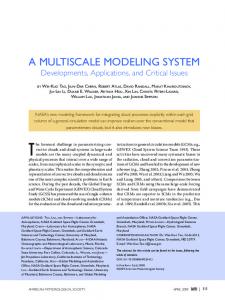
Figure 15. 2
A colorized model of 5 scale-domain manifolds based on annihilation events that have been extracted from a 200-layer SS stack (shown in Figure 4). The first scale models 1221 annihilation events, the second 152, the third 64, the fourth 28, and the final scale models 10 annihilation
4
events. The original study site (panchromatic image 500xy) is shown on the bottom to provide context. Colors are provided to aid visualization only.
6
37
Figures and Captions (Text only) 2 Figure 1.
Hierarchical structures showing the Object-Oriented ‘aggregation’ relationship.
Figure 2.
Hierarchical structures showing the Object-Oriented ‘generalization/specialization’ relationship.
Figure 3.
IKONOS sub-image and Study site map. (3a). A 500 x 500 pixel 4.0 m panchromatic image.
4
6
8
(3b). Map location of the image. Figure 4.
10
This illustrates a linear scale-space ‘stack’ or scale-space ‘cube’. The smallest scale (original image t0) is on the bottom, and the largest scale (t200 - most smoothed) is on the top. At the right side of the stack, the diffusive patterns of patches/objects through scale are visible
12 Figure 5.
Grey level blob mosaic illustrating different scale layers (t).
Figure 6.
Grey-level stack with opacity filters applied to illustrate the persistence of blob structures through
14
16
18
scale, with the original image on the bottom to provide context.
Figure 7.
Scale layer (t150), modeled as a 2.5D topographic surface. Contours represent an instance of flood-subsidence when two or more peaks become connected. These connected boundaries
20
become the ‘region of support’ for delineated blobs.
22
Figure 8.
Binary blob mosaic illustrating the same scale layers (t) as Figure 5.
24
Figure 9.
A hyper-blob stack composed of 2D binary blobs. For illustrated purposes only, each binary layer has been assigned a value equal to its scale. Thus dark values are on the bottom, while the
26
28
brightest value is at the top.
Figure 10.
Four generic blob-events. The gradient shaded disks represent the focal blob, i.e., the blob under analysis. The ‘?’ indicates that no blobs exist at this scale.
30 Figure 11. 32
A single, idealized hyper-blob illustrating four different blob-events: creations (C), merges (M), splits (S), and annihilations (A). The number of scales between SS-events represents the lifetime (Ltn) of a SS-blob. Five different Ltn are illustrated.
34 Figure 12. 36
Ranked blobs converted to individually queriable polygons. Note how the different colored polygons overlay each other making analysis non-trivial. Compare with Fig 3a.
38
Figure 13. 2
A conceptual model of three domain-level manifolds (layers) passing through SS events (red dots). Dark-toned disks represent the highest ranked blobs located within each of the three levels.
Figure 14.
Four new dual-instant blob events. The ‘?’ represents ‘no blobs found’ at these scales.
Figure 15.
A colorized model of 5 scale-domain manifolds based on annihilation events that have been
4
6
extracted from a 200-layer SS stack (shown in Figure 4). The first scale models 1221 annihilation events, the second 152, the third 64, the fourth 28, and the final scale models 10 annihilation
8
events. The original study site (panchromatic image 500xy) is shown on the bottom to provide context.
10