Journal of Marine Research, 58, 837–862, 2000
Journal of
MARINE RESEARCH Volume 58, Number 6
Modeling of the bottom water ow through the Romanche Fracture Zone with a primitive equation model—Part I: Dynamics by Bruno Ferron1, Herle´ Mercier1 and Anne-Marie Treguier1 ABSTRACT This paper investigates the dynamics of the Antarctic Bottom Water (AABW) ow through the Romanche Fracture Zone (RFZ) in a primitive equationmodel with a high horizontaland verticalresolution. Two examples of ows over simple bathymetries show that a reduced gravity model captures the essential dynamics of the primitive equationmodel. The reduced gravity model is then used as a tool to identify what are the bathymetricstructures(sills, narrows) that mostly constrainthe AABW ow through the RFZ. When only these structures are represented in the primitive equation model, the AABW ow is shown to be coherentwith observations(transports,density and velocity structures).
1. Introduction In the last few decades, the theory of hydraulic control has been widely applied to identify the basic mechanisms which control exchange ows between adjacent basins lled with different water properties (e.g., Hogg (1983) for the Vema Channel; Armi and Farmer (1985), Farmer and Armi (1988), Bryden and Kinder (1991) for the Gibraltar Strait; Pratt (1986) for the Iceland-Scotland Ridge; Oguz et al. (1990) for the Bosphorus Strait). These exchange ows are especially important for the dynamics of the deep component of the thermohaline circulation since passages are major constraints to the spreading of dense water masses. Moreover, ows through constrained passages are often associated with intense diapycnal mixing (e.g. Wesson and Gregg, 1994; Baringer and Price, 1997; Polzin et al., 1996; Ferron et al., 1998) which is required for closing the thermohaline circulation. 1. Laboratoire de Physique des Oce´ ans, IFREMER, BP 70, 29280 Plouzane´, France. email:
[email protected] 837
838
Journal of Marine Research
[58, 6
Therefore, these ows have to be represented or, at least, parameterized in general circulation models. This paper is dedicated to the dynamics of the eastward ow of Antarctic Bottom Water (AABW) through the Romanche Fracture Zone (RFZ) which connects the Brazil Basin to the Sierra LeoneAbyssal Plain and the GuineaAbyssal Plain (Fig. 1a). The topography of the RFZ is characterized by a complex succession of sills and narrows (Fig. 1b). The main sill is located at 13°458W and 0°518N and culminates near 4350 m. The ow has already been described and quanti ed in terms of transport and water mass mixing (Mercier et al., 1994; Polzin et al., 1996; Mercier and Morin, 1997; Mercier and Speer, 1998; Ferron et al., 1998).This study focuses on the ow dynamics and its representation in a primitive equation model. Downstream of the main sill, several characteristics of the ow suggest that the dynamics obey the hydraulic control theory. First, the cascade of the isopycnals (Fig. 2) indicates that the water experiences a transition from a state of high potential energy and low kinetic energy west of the main sill to a state of relatively low potential energy and high kinetic energy east of the main sill. Moreover, the isopycnal grounding downstream of the main sill (Fig. 2) suggests that an intense mixing occurs. Large local estimates of the vertical mixing and high level of turbulent kinetic energy dissipation (Polzin et al., 1996; Ferron et al., 1998) point out that, in the region immediately east of the main sill, shear instability may develop; this could be associated with internal hydraulic jumps located downstream of a hydraulic control point. In a hydraulically controlled ow, the transport depends critically on the characteristics of the bathymetry. Looking at Figure 1b, we cannot readily identify which narrow, sill or combination of the two will be the major constraints on the ow. In order to represent the RFZ in a primitive equation model, we need to represent the bathymetric structures that set the dynamics (transport, mixing) right without including the details of the bathymetry. In this paper we show that a reduced gravity model is an adequate and simple tool to identify those sills and narrows that will affect the ow. The structure of the paper is as follows. Descriptions of the primitive equation model and the reduced gravity model are given in Section 2. The two models, run with simple bathymetric con gurations, are compared in Section 3. We show that the dynamics of the reduced gravity model captures the essential dynamics of the primitive equation model. The reduced gravity model is used in Section 4 to identify the main topographic features (control points) that are expected to constrain the ow. Finally, in Section 5 the control points obtained in Section 4 are included in the primitive equation model bathymetric grid to run a ‘‘realistic’’ version. The primitive equation model solution obtained is compared to data in terms of transport, velocity and property distributions. 2. Model descriptions a. Con guration of the primitive equation model The primitive equation model (PEM) used is OPA (7th version, Delecluse et al., 1993) from the Laboratoire d’Oce´anographie DYnamique et de Climatologie (LODYC). OPA is
2000]
Ferron et al.: Dynamics of AABW eastward ow
839
Figure 1. (a) Bathymetry of the equatorial Atlantic Ocean from ETOPO5 Atlas. RFZ, CFZ, SLAP and GAP stand for the Romanche Fracture Zone, the Chain Fracture Zone, the Sierra Leone Abyssal Plain and the Guinea Abyssal Plain, respectively (upper frame); (b) Multi-beam echo sounder bathymetric map of the Romanche Fracture Zone taken during the Romanche 1 cruise showing the location of some bathymetric structures (lower frame).
840
Journal of Marine Research
[58, 6
Figure 2. Section of potential density anomaly (kg m2 3 ) referenced to 4000 dbars along the Romanche Fracture Zone axis (Romanche 1 cruise, Mercier et al., 1994).
a z-coordinate model which makes the hydrostatic, Boussinesq and incompressible assumptions. A rigid lid condition is prescribed at the surface. Equations are discretized on a C-grid with a second order nite difference scheme. A z-coordinate model was chosen despite the errors that may come from its step-like topography representation (Gerdes, 1993; Adcroft et al., 1997) because s -coordinate or isopycnic models have more severe limitations in the context of our study. A s -coordinate model (e.g., Haidvogel et al., 1991) is not appropriate due to the large cross-axis slopes of the fracture zone (they may exceed 40%) which are a source of hydrostatic inconsistency and pressure gradient error (e.g., Marchesiello et al., 1997). Likewise, although the representation of the ocean in an isopycnic model (e.g., Bleck and Chassignet, 1994) is close to the hydraulic model described in the next section, the parameterization of the diapycnal mixing in isopycnic models is not as advanced as parameterizations of mixing in z-coordinate models yet (DYNAMO, 1997). The OPA con guration consists of a closed basin (1430 km 3 830 km) composed of two sub-basins (depth 5 5500 m) which are separated by a ridge (depth 5 3180 m) (Fig. 3a). The fracture zone (depth # 4330 m) created in the middle of the ridge is aligned with the x-axis. It allows an eastward ow of dense waters from the Brazil Basin (0 km # x # 400 km) to the African Basin (1000 km # x # 1400 km) maintained by the deep pressure gradient created by the difference in density at a given depth between the bottom water in the Brazil Basin and that in the African Basin. Like the RFZ, the x-axis of the model is rotated by 10° from the equator.
2000]
Ferron et al.: Dynamics of AABW eastward ow
841
Figure 3. (a) 3D view of the primitive equation model bathymetry (upper frame); (b) Variables of the 112 layered hydraulic model (lower frame).
The horizontal grid of the model is nonuniform; the horizontal resolution is 10 km 3 5 km (x 3 y) around the fracture zone axis, and falls down to 20 km 3 10 km away from the fracture zone. We will show that this horizontal resolution is sufficient to represent most of the bathymetric structures of the RFZ. The vertical resolution is 20 m near the depth of
842
Journal of Marine Research
[58, 6
the main sill (i.e., where the topography and the baroclinic pressure gradient are expected to be important for driving the ow), while the vertical resolution is 1000 m for the rst level and 220 m for the deepest level. A free-slip condition is prescribed at the lateral boundaries. This is a crucial parameter for ows in narrow passages. A no-slip condition makes the results highly dependent on the no-slip parameterization used but also on the horizontal eddy diffusion coefficient. With only 5 km resolution in the transverse direction, we cannot resolve the boundary layer along the sidewalls so that a free-slip condition is numerically more appropriate. The horizontal diffusion is a Laplacian with an eddy diffusion coefficient Kh 5 20 m2 s2 1. A quadratic friction is used to represent bottom friction with a drag coefficient Cd 5 1.5 3 102 3. The vertical mixing is parameterized using Blanke and Delecluse’s (1993) turbulent kinetic energy closure scheme. In this closure model [level 2.5 in Mellor and Yamada (1982) classi cation], the change in the turbulent kinetic energy (a prognostic variable) of the ow depends on its advection, its vertical diffusion, its production from the mean velocity shear, its transfer to potential energy and its dissipation. In order to reproduce the observed pressure gradient between the western and eastern basins, the Brazil and African basins’ temperature and salinity pro les are initialized with CTD pro les measured at the entrance and the exit of the fracture zone respectively (Fig. 4a). Inside the fracture zone, a horizontal linear interpolation is used to produce a smoothed density gradient. Initially, the pressure gradient is zero above the summit of the ridge. Temperature and salinity pro les are restored to initial conditions below the summit of the ridge in the Brazil Basin since this basin represents a reservoir for the dense waters. Note that when there is no relaxation, waves propagating upstream of the control point do not modify signi cantly the upstream energy of the ow. Rather, the upstream energy is slowly modi ed by the volume ux through the passage, which leads to unstationary transports (decreasing trend) since the reservoir is too small for the bottom transport in the fracture zone. Hence, restoring conditions are necessary to maintain the upstream energy observed in the data. No restoring conditions are prescribed in the downstream basin as water mass characteristics there depend on the dynamics of the ow within the fracture zone. The only forcing applied is the baroclinic pressure gradient that exists along the RFZ axis. b. The reduced gravity model We consider a one-dimensional stationary model composed of two layers (Fig. 3b). The uid is stably strati ed such that r 1 , r 2, r 2 is the density of the lower (active) layer. The upper layer is at rest. h denotes the thickness of the active layer, b the height of the bathymetry above the level z 5 2 H (where z is the vertical coordinate, positive upward), l the width of the fracture zone and u the velocity of the active layer. These variables are functions of the distance along the fracture zone axis x (positive eastward). The bottom friction is written as a quadratic operator with a drag coefficient Cd 5 1.5 3 102 3 (Pratt,
2000]
Ferron et al.: Dynamics of AABW eastward ow
843
Figure 4. Density along the fracture zone axis at (a) initialization (t 5 0) and (b) after adjustment (t 5 90 days); (c) temporal evolution of the transport of water colder than 1.9°C across four sections of the fracture zone.
Journal of Marine Research
844
[58, 6
1986; Wajsowicz, 1993). As changes in topographic height along the fracture zone axis are smooth (slopes do not exceed 5%), the vertical acceleration is weak so that the uid can be considered hydrostatic. The rotation is removed from the problem since the RFZ is located at the equator (the internal Rossby radius is greater than 100 km whereas the mean fracture zone width is 20 km). The momentum equation reads: du
u where g8 5
[(r
2
2
5
dx
2 g8
d dx
h) 2
Cd
u2
(1)
h
r 1)/r 2]g is the reduced gravity. The continuity equation is: dQ dx
where Q 5
(b 1
5
0
(2)
uhl is the transport of the active layer. Combining 1 and 2 yields: (F 2 2
1)
du dx
5
2
u db h dx
u dl 1
l dx
2
Cd
u3
(3)
g8h 2
where F 5 u/( g8h) 0.5 is the Froude number. We seek a controlled solution that produces an asymmetrical interface over a symmetrical obstacle (that is, a solution for which the interface between the active and passive layers spills down to the valley located downstream of the sill as shown in Figure 3b; an important asymmetry as observed in the data downstream of the main sill (Fig. 2) cannot be achieved with a realistic bottom drag; indeed, we would need Cd 5 0.1 to match the observed asymmetry which is too large by two order of magnitude). A hydraulic control point occurs where F 5 1 (e.g., Gill, 1977). At this particular point, the right-hand side of Eq. 3 must vanish for the solution to be nite: db dx
h dl 2
l dx
5
2 Cd
when
F5
1.
(4)
As b and l are set by the bathymetric observations, Eq. 4 is used to nd the locations of the hydraulic control points. At these points, the derivatives of Eqs. 1 and 2 with respect to x can be combined to yield: 3ul
1 dx2 1 du 2
1
3Cdg8l 1
2u 2
dx2 dx
dl du 1
g8ul
d 2b dx
2 2
u3
d 2l dx
1 2
2
l 1 dx2
u 3 dl
2
1
Cdg8u
dl dx
5
0
(5)
which can be solved for du/dx. To determine the position of the interface for a given g8 and Q, we start from the point of hydraulic control located with Eq. 4. At this critical point, if the width is constant, the condition F 5 1 and Eq. 2 allows us to calculate the velocity uc and the interface height hc; if the width varies, Eq. 4 provides hc and Eq. 2 gives uc. Then, Eq. 5 is used to calculate the rst derivative of u at the control point and Eq. 2 that of h.
2000]
Ferron et al.: Dynamics of AABW eastward ow
845
From the control point, we can integrate the solution upstream and downstream using Eqs. 3 and 2 to solve for du/dx and dh/dx, respectively. Matching the supercritical ow to the subcritical ow of the downstream basin is achieved via a hydraulic jump. We consider a simple hydraulic jump model based on conservations of mass and momentum. Since the hydraulic jump dissipates much more energy than the bottom friction does over one grid point, Cd can be neglected and we can use the classical expression (e.g. Turner, 1973; Baines, 1995): hd hu
5
1 2
[2 1 1
(1 1
8F 2u ) 1/2 ]
(6)
where h is the layer thickness, F the Froude number and subscripts u and d denote the upstream and downstream points closest to the jump. Eq. 6 is used for determining the position of the hydraulic jump that will give the right position of the interface in the downstream basin. Equations and properties of controlled ows have been discussed by several authors (e.g., Gill, 1977; Pratt, 1986) to whom the reader is referred for further discussion. 3. Comparison of the reduced gravity model with the primitive equation model In this section, we show that the reduced gravity model captures the basic physics of the primitive equation model. This is done by comparing the behavior of the models when we assume that the continuously strati ed ow of the PEM can be approximated as a two layer system. Two academic problems which are relevant to the RFZ are considered: a ow over a sill and a ow over a sill combined with a narrow. For both cases and both models, the sill has a Gaussian shape. The cross-section of the fracture is rectangular. In order to set up the reduced gravity model in a con guration comparable to that of the PEM solution, we need information about the strati cation g8 and the transport Q. To determine g8 and Q, we select a potentially controlled isopycnal from the PEM solution, that is an isopycnal which is asymmetrical with respect to the sill. Moreover, since we require that the active layer of the reduced gravity model represents the over owing layer in the PEM, the selected isopycnal has to be close to the level of the reversal of the ow present in the PEM. Once the isopycnal from the PEM is selected, we calculate the transport Q below it from the PEM velocity eld. The transport of the active layer of the reduced gravity model is set to the same value Q. In the following, the variables of the PEM indexed with 2 are averaged from the sea oor up to the selected isopycnal, and those indexed with 1 are averaged from the selected isopycnal up to the summit of the ridge where the PEM velocity eld shows slow motions. The reduced gravity g8 is calculated using the vertically averaged densities in those two layers. g8 and Q are taken upstream of the point of control where their values are nearly constant since the vertical mixing of the PEM is weak. Contrary to the reduced gravity model whose upper layer is at rest, there is no passive layer in the PEM. Rather, the mean velocity u1 does not vanish since most of the
846
Journal of Marine Research
[58, 6
corresponding layer is located in the returning ow which closes the mass balance. However, it will be shown that the Froude numbers F1 and F2 from the PEM satisfy: F1 ½ F2. Hence, the condition for hydraulic control in the presence of two active layers F1 1 F2 5 1 (e.g. Armi, 1986) can be safely approximated as F2 5 1. Thus, it is sound to consider a gravity model with one active layer only. a. Experiment with a sill In this rst experiment, we consider a sill of Gaussian shape sets at the location of the RFZ main sill (x 5 855 km). Its height is equal to that of the main sill of the RFZ (4350 m). The cross-section of the fracture zone is rectangular. Its width is constant and set to 20 km, which is comparable to the mean width of the RFZ. Figures 4a and b show the evolution of the isopycnals along the RFZ axis in the PEM between time t 5 0 and t 5 90 days, respectively. This is a lock exchange experiment. Internal waves propagate upstream and downstream of the main sill during the adjustment phase. Dense waters from the Brazil Basin move east toward the African Basin, shifting the horizontal bottom pressure gradient eastward, up to the sill location. As the model evolves from the initial condition, a zonal pressure gradient opposite to that set at deeper depths builds around 3000 meters to maintain the returning ow necessary to close the mass budget (note again that the whole domain is closed, so are each sub-basin below the ridge depth apart from the fracture zone). At t 5 90 days, the time evolution is slow and a quasi-stationary state is reached. The AABW is de ned, in the primitive equation model, as the water mass whose potential temperature is colder than 1.9°C. Looking at the AABW transport time series (Fig. 4c), the AABW transport is quasi-stationary after 90 days. When the adjustment of the model is completed, the transport is nearly equal to 1.8 3 106 m3 s2 1 from the entrance (x 5 415 km) of the fracture zone up to the main sill (x 5 855 km). Downstream of the main sill, the transport increases signi cantly (1 0.6 3 106 m3 s2 1 ) between the main sill and the exit (x 5 1000 km): deep waters are entrained in the AABW current. The evolution of the isopycnals along the RFZ axis as modeled in the PEM after six months of simulation shows the dense water spillover just immediately downstream of the summit of the sill (Fig. 5a). In order to calibrate the reduced gravity model, we select in the PEM the isopycnal s 4 5 45.89 kg m2 3. From the PEM we nd d r 5 0.1 kg m2 3 and Q 5 1.75 3 106 m3 s2 1. The interface position as diagnosed by the reduced gravity model is shown in Figure 5a (thick dashed line). Up to the summit of the sill, this interface closely follows the selected isopycnal of the PEM (s 4 5 45.89 kg m2 3 ). For both models, the asymmetry center of the shape of the interface occurs near the summit of the sill as expected from the hydraulic control theory. Downstream of the sill, we note a divergence between the behavior of the PEM isopycnal and that of the reduced gravity model interface. The isopycnal of the PEM is detrained due to the vertical mixing that occurs downstream of the sill while the reduced gravity model does not include mixing. The vertical mixing in the PEM is produced by the
2000]
Ferron et al.: Dynamics of AABW eastward ow
847
Figure 5. (a) Comparison of the behavior of the PEM selected isopycnal (45.89 kg m2 3 ) and the corresponding reduced gravity model interface (dashed thick line) for the sill experiment case. Thin dashed lines show changes of 6 10% in the density difference g8 of the reduced gravity model (upper frame). The dotted curve indicates when a hydraulic jump is included in the reduced gravity model. (b) Same as upper panel but for the sill and narrow case (lower frame).
848
Journal of Marine Research
[58, 6
large vertical shear of horizontal velocities that exists downstream of the sill. The parameterization of the vertical mixing in the primitive equation model is beyond the scope of this paper; it will be the subject of a subsequent study. If we change d r by 6 10% in the reduced gravity model, we get the dashed thin lines shown in Figure 5a. The interface position is only weakly sensitive to this change since hc is a function of g82 1/3. The evolution of the Froude numbers in the PEM and the reduced gravity model is displayed in Figure 6a. F2 highly increases downstream of the sill summit (x 5 850) km, whereas F1 always stays below 0.08. Hence, we can safely compare F2 to F, the latter being the Froude number of the active layer of the reduced gravity model. The variations of F2 and F closely follow each other up to the region where the Froude numbers approach 1. In the reduced gravity model, the hydraulic control point (F 5 1) is found slightly downstream of the summit of the sill. In the PEM, the bottom layer, which also exhibits a hydraulic control point (F2 5 1) downstream of the summit of the sill, is, on average, as strongly accelerated as the active layer of the reduced gravity model at the approach of the sill. Downstream of the sill, the curves diverge. In the reduced gravity model, the active layer accelerates until the quadratic friction removes enough kinetic energy from the ow and contributes to a decrease in F. In the PEM, two physical parameterizations are responsible for the decrease in F2: the quadratic friction at the bottom and most importantly the vertical mixing. The vertical mixing both dissipates kinetic energy and transfers kinetic energy into potential energy. Thus, F2 does not reach the high values of F. Figures 7a and b show the vertically integrated kinetic and potential energies in the lower layer of both the PEM and the reduced gravity model, respectively. Downstream of a hydraulic control point, the uid experiences a transfer of potential energy to kinetic energy. This behavior is observed for both models which present similar conversion rates of potential to kinetic energies. However, as shown previously, mixing limits this conversion downstream of the sill in the PEM. Indeed, part of the kinetic energy of the supercritical ow is converted back to potential energy through the mixing mechanism. The sudden increase in potential energy at x 5 920 km could be interpreted as the signature of a hydraulic jump. The location of the hydraulic jump in the reduced gravity model is also close to x 5 920 km (Figs. 5a and 7b). In the presence of such a jump, the kinetic energy decreases too rapidly in the reduced gravity model (Fig. 7a), giving a Froude number weaker than in the PEM. (Fig. 6a). Note that this comparison has to be considered with caution since g8, constant in our model, should change downstream of this hydraulic jump. b. Experiment with a sill and a narrow Narrows are another potential source of hydraulic control for ow through passages. In this experiment, a narrow is added 50 km (5 grid points) downstream of the sill (same sill as that used previously). At the narrow location (x 5 905 km), the width is equal to 5 km over 20 km along the fracture axis. The narrow extends up to the summit of the ridge. Elsewhere in the fracture zone the width is kept constant (20 km). The initial strati cation
2000]
Ferron et al.: Dynamics of AABW eastward ow
849
Figure 6. (a) Comparison of Froude numbers for the sill experiment case (upper frame); F1: PEM Froude number of the returning ow layer (dash-dotted); F2: PEM Froude number of the bottom over owing layer (solid); F: Froude number of the active layer (thick dashed: without hydraulic jump; thin dashed: with a hydraulic jump). (b) Same as upper panel but for the sill and narrow case (lower frame).
in the PEM is the same as for the previous experiment. After the adjustment period, the AABW transport in the PEM is reduced compared to the previous case. Figure 5b presents the density anomaly eld of the PEM after six months of run. The presence of the narrow uplifts the isopycnals by several tens of meters between 3600 m and 4000 m. In this depth range, the strati cation has weakened compared to initial conditions.
850
Journal of Marine Research
[58, 6
Figure 7. Comparison of (a) the vertically integrated kinetic energy (upper frame) and (b) the vertically integrated potential energy (lower frame) for the sill experiment case. In the PEM model (solid), the integration starts from sea oor up to the selected isopycnal. In the reduced gravity model (thick dashed: without hydraulic jump; thin dashed: with a hydraulic jump) it goes from the sea oor up to the interface.
The most striking feature is the eastward shift of the isopycnal cascade. In the rst experiment, the cascade begins immediately downstream of the summit of the sill (Fig. 5a), whereas in the present case, the cascade is shifted farther downstream, at the position of the narrow. s 4 5 45.885 kg m2 3 is now the selected isopycnal which sets d r and Q to 0.1 kg m2 3 and 1.24 3 106 m3 s2 1, respectively. In the reduced gravity model, the hydraulic control point is located between the sill and the narrow (Eq. 4). For low transports of the active layer, the hydraulic control point is
2000]
Ferron et al.: Dynamics of AABW eastward ow
851
Figure 8. Same as Figure 10 but for the sill and narrow case.
located immediately downstream of the summit of the sill. If we increase the transport, the hydraulic control position moves slightly eastward until the transport reaches 0.8 3 106 m3 s2 1 and then jumps immediately upstream of the narrow for higher transport values. Running the reduced gravity model with the transport of the PEM gives a hydraulic control located in the upstream vicinity of the narrow (Fig. 5b). The reduced gravity model interface behavior looks like that of the PEM selected isopycnal. However, at the entrance of the fracture zone, the interface depth is 70 m deeper than the selected isopycnal (10 m deeper in the rst experiment). As for the Froude number comparison (Fig. 6b) and the potential/kinetic energies (Figs. 8a–b), the comments made for the rst experiment also apply.
Journal of Marine Research
852
[58, 6
The reduced gravity model shows a close behavior to that of the PEM for subcritical ows up to the point of criticality. That is, the reduced gravity model dynamics capture the basic balance of the dynamics of the complex PEM (exchange of potential to kinetic energy, position of the control points). On the supercritical part of the ow, the two models diverge since the vertical mixing is only included in the PEM. Compared to the observations that reported 0.66 6 0.14 3 106 m3 s2 1 of AABW transport through the RFZ (Mercier and Speer, 1998), the rst two experiments respectively give AABW transports that are 2.7 and 1.8 times larger than the observed transport. Thus, we cannot simply represent such a passage by a sill and narrow of rectangular cross-section that represents the average shape of the RFZ. To get transports and heat uxes right, we need to identify and represent as accurately as possible (according to the resolution of the PEM) the cross-sectional structures of the most constraining bathymetric events. Since the reduced gravity model has displayed the same hydraulic control regions as the PEM in the rst two experiments, we use it in the next section to identify which are, in the RFZ bathymetry, the structures that mostly constrain the AABW ow.
4. Identi cation of the main topographic constraints A database describing the variation of the RFZ width l along its axis as a function of the height h above the bottom was created. It is based on 25 transverse bathymetric sections located at key points (narrows, sills, valleys) of the fracture zone (Fig. 9b). As seen in the previous section, the location of a hydraulic control point depends on the transport of the active layer. Variations in the strength of the transport may shift the hydraulic control point from one section to another. Hence, it appears necessary to look for potential controlling sections within a range of realistic transports. To perform this search, we use the speci c property that a controlled over ow has the minimum energy among all possible (subcritical and supercritical) solutions. Indeed, the integration of Eq. 1 as a function of x yields the Bernoulli constant B of the ow (since friction only slightly offsets the hydraulic control location we neglect Cd ): B5 Using F 5
u/(Î g8h) and Q 5 B(F) 5
2u 2 1
g8(b 1
1
h) 5
constant
(7)
uhl, Eq. 7 can be rewritten as:
1 l2
1 g8Q 2
2/3
(F 4/3 1
2F 2
2/3
)1
g8b.
From Eq. 8, if Q is constant, we see that B(F) is minimum (dB/dF 5 such a critical ow we then have: Bc 5
21 l 2 3 g8Q c
2/3
1
g8bc
(8) 0) when F 5
1. For
(9)
2000]
Ferron et al.: Dynamics of AABW eastward ow
853
Figure 9. (a) Minimum energy (Bernoulli function) that the ow needs to pass the different sills and contractions for different transports (1 Sv 5 1 3 106 m3 s2 1 ) (upper frame); (b) Width of the RFZ at 4000 m (dark gray) and height above the deepest point of the passage (light gray) (lower frame).
854
Journal of Marine Research
[58, 6
where subscript c indicates that variables are expressed at the control point. Bc represents the energy at a control point for a constant transport Q and a given strati cation g8. Variations of Bc as a function of transport and along-axis distance x are displayed in Figure 9a. Given Q, we identify from Figure 9a the most constraining bathymetric structure as the feature which sets the maximum value of Bc within the fracture zone. For instance, if Q 5 0.2 3 106 m3 s2 1, the energy of the ow should be equal to the value of Bc at the main sill (1.08 J kg2 1) for the ow to be controlled.A ow with a weaker energy cannot exist since it would not be able to pass over the main sill. A ow with a larger energy may exist but, it is either subcritical or supercritical everywhere in the fracture zone. Hence, for a controlled ow with a transport of 0.2 3 106 m3 s2 1, the main sill is the most constraining section. The reduced gravity model exhibits only one hydraulic control point (main narrow or main sill, Fig. 9). In the presence of several narrows and sills and given the existence of internal hydraulic jumps, a ow of transport Q may be controlled at several locations. This is not permitted in our reduced gravity model. However, it gives partial information on what may happen in a more realistic representation of the ow. For instance, for Q 5 2.7 3 106 m3 s2 1, the reduced gravity model shows that the main sill section requires slightly less energy than the main narrow for the ow to cross it. In this case, the ow could be controlled at the main narrow, become supercritical downstream of the narrow, then go through a hydraulic jump and dissipate energy, come back to a subcritical state downstream of the jump, be again controlled at the main sill with another hydraulic jump downstream of the sill to match the subcritical conditions of the downstream basin (state described in Pratt, 1986; Fig. 4d dashed line). Figure 9a basically shows that, for low transports (Q 5 0.2 3 106 m3 s2 1 ), the uid is mainly sensitive to the bathymetric height rather than to the changes in width (Fig. 9b) and the main sill is the point of control. For large transports (Q 5 3.2 3 106 m3 s2 1 ), the narrows overcome the changes in height in the degree of constraint of the uid and the main narrow is the point of control. For intermediate transports, four bathymetric structures exhibit close values of Bc: the main narrow, the current meter sill, the main sill and its downstream narrow. With the possible existence of internal hydraulic jumps and multiple control points, it appears necessary to take into account these four bathymetric structures in a ‘‘realistic’’ PEM con guration. 5. Application to the primitive equation model We now include in the PEM the four bathymetric structures identi ed in the previous section. The vertical and horizontal resolutions are the same as those used in the rst two experiments. The bathymetry is adjusted so that the area below a given model level is as close as possible to the real area of the four bathymetric sections (Fig. 10). a. Temperature distribution and velocity eld Figure 11 presents the observed and modeled potential temperature distribution in the RFZ. As suggested by the reduced gravity model for transports in the range of
2000]
Ferron et al.: Dynamics of AABW eastward ow
855
Figure 10. PEM bathymetry enlargement showing the four bathymetric structures of the fracture zone.
0.6–1 3 106 m3 s2 1 (Fig. 9) as diagnosed from the PEM, the cascade of the isopycnal occurs downstream of the main sill in this PEM run. This is in agreement with the observed temperature eld. A comparison between measured vertical pro les of velocity and corresponding pro les of the PEM is done at the location of the main sill and the downstream plateau (Fig. 12). Below 3600 m, where the vertical resolution is higher than 250 m, the PEM velocity pro le is particularly close to the LADCP and HRP pro les both at the main sill and the plateau. A weak returning ow is present between 2700 m and 3500 m both on the LADCP data and in the PEM. Note that the HRP data do not give the absolute velocity but provide the vertical gradient of horizontal velocity. b. AABW transport Figure 13a shows the AABW transport at four different cross-sections of the RFZ. After an adjustment period of three months, the AABW transport displays no long-term tendency. In the last three months of run, the AABW transport is constant from the entrance up to the current meter region. Its value of 0.75 3 106 m3 s2 1 is within the standard deviation of the observed AABW transport (shaded area on Fig. 13a) measured at the so-called current-meter sill (Mercier and Speer, 1998). Thus, the implementation in the
856
Journal of Marine Research
[58, 6
Figure 11. (a) Observed potential temperature cut along the RFZ axis (upper frame); (b) Modeled potential temperature cut along the RFZ axis (lower frame).
2000]
Ferron et al.: Dynamics of AABW eastward ow
857
Figure 12. Comparison of observed and modeled vertical pro les of the axial velocity at the main sill (left panel) and the downstream plateau (right panel).
PEM of the four bathymetric structures identi ed with the reduced gravity model results in a transport of AABW in the PEM coherent with the observations. Between the current meter sill and the main sill of the PEM, some entrainment (1 0.06 3 106 m3 s2 1 ) occurs. The entrainment is larger downstream of the main sill since the AABW transport increases by 0.15 3 106 m3 s2 1. The importance of each bathymetric feature is inferred from Table 1. In these experiments, one or several bathymetric features is removed from the PEM bathymetry while keeping other sills and narrows untouched. The reduced gravity model indicates that for a transport of 0.75 3 106 m3 s2 1, the ow is controlled by the main sill (Fig. 9). Hence, as long as the main sill remains, the AABW transport should be constant. Accordingly, the PEM shows (Table 1, column 1–4) that the AABW transport increases by a maximum of 20% which occurs when the main narrow is removed. When the main sill is removed in the PEM, the reduced gravity model (Eq. 9) may be used to predict what is the new control point and the associated AABW transport. Indeed, the energy Bc , 1.17 J/kg found at the main sill (control point) for a transport of 0.75 3 106 m3 s2 1 (Fig. 9) corresponds to the
858
Journal of Marine Research
[58, 6
Figure 13. (a) AABW transports across four sections of the fracture zone (upper frame). x 5 415 km: entrance of the fracture zone; x 5 735 km: current-meter sill section; x 5 855 km: main sill section; x 5 985 km: exit of the fracture zone; the shaded area is the AABW transport (averaged over two years) and its standard deviation measured at the current-meter sill. (b) transports by potential temperature classes and the corresponding measured transports (averaged over two years) (horizontal thick lines, lower frame).
2000]
Ferron et al.: Dynamics of AABW eastward ow
859
Table 1. Transports of AABW measured for different bathymetric con gurations of the PEM (unit 5 1 3 106 m 3 s2 1 ). The simulation of reference makes use of the four bathymetric structures identi ed in Section 4. Column 2–5 are experiments where only one structure is removed from the bathymetry (other bathymetric features untouched). In the experiment of column 6, all the bathymetric structures are removed except the main narrow.
Reference
Without main narrow
Without currentmeter sill
Without downstream narrow
Without main sill
With only main narrow
0.75
0.9
0.85
0.75
1.25
1.6
energy B0 available in the upstream reservoir (the dissipation of energy is weak between the entrance of the RFZ and the main sill so that B0 , Bc ). In the PEM, B0 does not vary with time and is not in uenced by the RFZ dynamics since B0 is imposed by the restoring condition in the reservoir of AABW. When the main sill is removed and for a B0 , 1.17 J/kg, Eq. 9 predicts that the new control point is the current meter sill and that the AABW transport reaches 1.4 3 106 m3 s2 1. The removal of the main sill from the PEM bathymetry (Table 1, column 5) results in an AABW transport of 1.25 3 106 m3 s2 1 (1 70% compared to the reference run) and a cascade of isopycnals located at the current meter sill revealing it as a control point. If all the bathymetric structures but the main narrow are removed, Eq. 9 predicts that the ow is controlled at the main narrow and the AABW transport is 1.6 3 106 m3 s2 1. When run with only the main narrow (Table 1, column 6), the PEM exhibits a control at the narrow and a transport of 1.65 3 106 m3 s2 1 (1 120%). Comparing the PEM transports by potential temperature classes, at the current meter sill, to their corresponding observed values (Fig. 13b) con rms the good performance of this run except for the bottom most waters (u , 0.9°C). This result can be explained by the difficulties that arise from the PEM representation of the bathymetry. Indeed, the real area of the deepest layers is small compared to that of the shallower layers. Hence, choosing between an ocean point or a land point at the level of the deepest layers may increase or decrease the area by several tens of percent. Ipso facto, the transport of the bottom most layers will be sensitive to the representation of the topography. 6. Discussion Given the complexity of the RFZ bathymetry composed of a succession of sills and narrows, a reduced gravity model proves to be a useful tool for identifying the bathymetric structures that mostly constrain the ow of AABW through the RFZ. This is a crucial step for the representation of such passage in general circulation models. The omission or misrepresentation of such a bathymetric constraint, and especially of the control section, would result in incorrect exchange of water masses between adjacent basins. This would certainly also lead to a bad representation of the vertical/diapycnal mixing rates since this mixing, often intense in these types of regions, highly depends on the vertical shear generated by the acceleration of the ow at the control point.
860
Journal of Marine Research
[58, 6
The reduced gravity model does not take into account the vertical mixing that occurs downstream of the main sill, where the ow is supercritical. The comparisons done between the reduced gravity model and the PEM on simple bathymetries have clearly shown the divergence due to the parameterization of the vertical mixing of the PEM. The PEM solution, which uses a high resolution, is remarkably close to observed transports, velocity pro les and density distribution.A vertical resolution coarsened to 200 meters (instead of 20 m) without signi cantly changing the main sill depth and geometry does not change the transport of AABW by more than 15%. However, transports by temperature classes may vary by more than 50% since it is not always possible to maintain the observed area below a model level. The higher the model level in the water column, the more stable the transport below this level. Coarsening the horizontal resolution to values used for circulation studies at larger scales and keeping the sill depth unchanged is more problematic since the resulting widening of the RFZ would result in an increase of the AABW ow in the adjustment phase. This would in turn decrease the initial potential energy of the AABW in the reservoir (Brazil Basin) compared to observations. From a general circulation point of view, this cannot be satisfying since it would also decrease the export of AABW toward the North Atlantic (and it would also probably change the interior circulation of AABW in the Brazil Basin). Hence, for resolutions that do not permit a good representation of the width of the most constraining section, a solution might be to include an adequate no-slip condition on the side walls to have a reasonable bottom water transport and therefore maintain the observed upstream energy. Ideally, one would like to relate the PEM solution to a continuously strati ed theory rather than a reduced gravity one. Pratt et al. (2000) extended the Taylor-Goldstein equation to calculate the continuous dynamical modes of long waves for the case of straits having arbitrary cross-sections. In their study, the hydraulically controlled state of the ow is assessed by looking at where the long-wave phase speeds c is 0 (which corresponds with F 2 5 1 Û U 2 2 c 5 0 with c 5 Î gh in our reduced gravity model). They showed that, in the case of an exchange out ow (the velocity in the strait changes its sign with depth), a hydraulic control point may occur only if the Richardson number Ri 5 min (N(z) 2/ ( zU(z)) 2 ) is , 14. Repeated pro les of LADCP measured downstream of the main sill exhibit regions where Ri , 14 and are associated to an intense vertical mixing (Polzin et al., 1997; Ferron et al., 1998). However, the application of Pratt et al.’s (2000) theory to this AABW ow does not give any conclusive results. It is, therefore, satisfying to see that, despite its simplicity, our reduced gravity model is useful to understand the behavior of the continuously strati ed model, and to select the bathymetric features that have the greatest in uence on the transport. Acknowledgments. This work was supported in part by the Centre National de la Recherche Scienti que (CNRS/INSU), the Institut Franc¸ais de Recherche pour l’Exploitation de la Mer (IFREMER) through the French Programme National d’Etude de la Dynamique du Climat
2000]
Ferron et al.: Dynamics of AABW eastward ow
861
(PNEDC). BF was supported by IFREMER and CNRS, AMT and HM by CNRS. Numerical experiments of the primitive equation model were made at the Institut du De´veloppement et des Ressources en Informatique Scienti que (CNRS/IDRIS). We gratefully acknowledge stimulating discussions with Gurvan Madec and Dr Peter Killworth. We wish to thank reviewers for their comments which helped to improve the original manuscript signi cantly.
REFERENCES Adcroft A., C. Hill and J. Marshall. 1997. Representation of topography by shaved cells in a height coordinate ocean model. Monthly Weather Rev., 125, 2293–2315. Armi, L. 1986. The hydraulics of two owing layers with different densities. J. Fluid Mech., 163, 27–58. Armi, L. and D. Farmer. 1985. The internal hydraulics of the Strait of Gibraltar and associated sills and narrows. OceanologicaActa, 8, 37–46. Baines, P. G. 1995. Topographic effects in strati ed ows. Cambridge Univ. Press, 482 pp. Baringer, M. O. and J. F. Price. 1997. Mixing and spreading of the Mediterranean out ow. J. Phys. Oceanogr., 27, 1654–1677. Blanke, B. and P. Delecluse. 1993. Variability of the tropical Atlantic Ocean simulated by a general circulation model with two different mixed-layer physics. J. Phys. Oceanogr., 23, 1363–1388. Bleck, R. and E. Chassignet. 1994. Simulating the ocean circulation with isopycnic coordinate models, in The Oceans: Physical-Chemical Dynamics and Human Impact, S. K. Majumdar, E. W. Miller, G. S. Forbes, R. F. Schmalz and A. A. Panah, eds., The Pennsylvania Academy of Science, 17–39. Bryden, H. L. and T. H. Kinder. 1991. Steady two-layer exchange through the Strait of Gibraltar. Deep-Sea Res., 38, (Suppl. 1), S445–S463. Delecluse, P., G. Madec, M. Imbard and C. Levy. 1993. OPA, version 7, Ocean General Circulation Model, Reference Manual. Rapport interne LODYC, 113 pp. Dynamo Group. 1997. Dynamics of North Atlantic models: Simulation and assimilation with high resolution models. Institut Fu¨r Meereskunde, 294, 334 pp. Farmer, D. and L. Armi. 1988. The ow of Atlantic water through the Strait of Gibraltar. Prog. Oceanogr., 21, 1–105. Ferron, B., H. Mercier, K. G. Speer, A. E. Gargett and K. L. Polzin. 1998. Mixing in the Romanche Fracture Zone. J. Phys. Oceanogr., 28, 1929–1945. Gerdes, R. 1993. A primitive equation ocean circulation model using a general vertical coordinate transformation. 1. Description and testing of the model. J. Geophys. Res., 98, 14,683–14,701. Gill, A. E. 1977. The hydraulics of rotating-channel ow. J. Fluid Mech., 80, 641–671. Haidvogel, D. B., J. L. Wilkin and R. E. Young. 1991. A semi-spectral primitive equation ocean circulation model using vertical sigma and orthogonalcurvilinear horizontal coordinates. J. Comp. Phys., 94, 151–185. Hogg, N. G. 1983. Hydraulic control and ow separation in a multi-layered uid with applications to the Vema Channel. J. Phys. Oceanogr., 13, 695–708. Marchesiello, P., B. Barnier and A. P. de Miranda. 1997. A sigma-coordinate primitive equation model to study the circulation in the South Atlantic. Part II: Meridional transports and seasonal variability. Deep-Sea Res., 45, 573–608. Mellor, G. L. and T. Yamada. 1982. Development of turbulence closure model for geophysical uid problems. Rev. Geophys. Space Phys., 20, 851–875. Mercier, H. and P. Morin. 1997. Hydrography of the Romanche and Chain Fracture Zones. J. Geophys. Res., 102, 10,373–10,389.
862
Journal of Marine Research
[58, 6
Mercier, H. and K. G. Speer. 1998. Transport of bottom water in the Romanche Fracture Zone and the Chain Fracture Zone. J. Phys. Oceanogr., 28, 779–790. Mercier, H., K. G. Speer and J. Honnorez. 1994. Flow pathways of bottom water through the Romanche and Chain Fracture Zones. Deep-Sea Res., 41, 1457–1477. Oguz, T., E. Ozsoy, M. A. Latif, H. I. Sur and U. Unluata. 1990. Modeling of hydraulically controlled exchange ow in the Bosphorus Strait. J. Phys. Oceanogr., 20, 945–965. Polzin, K. L., K. G. Speer, J. M. Toole and R. W. Schmitt. 1996. Intense mixing of Antarctic Bottom Water in the equatorialAtlantic Ocean. Nature, 380, 54–57. Pratt, L. J. 1986. Hydraulic control of sill ow with bottom friction. J. Phys. Oceanogr., 16, 1970–1980. Pratt, L. J., H. E. Deese, S. P. Murray and W. Johns. 2000. Continuous dynamical modes in straits having arbitrary cross sections, with application to the Bab al Mandab. J. Phys. Oceanogr., 30, 2515–2534. Turner, J. S. 1973. Buoyancy Effects in Fluids. Cambridge Univ. Press, 368 pp. Wajsowicz, R. 1993. Dissipative effects on inertial ows over a sill. Dyn. Atmos. Oceans, 17, 257–301. Wesson, J. C. and M. C. Gregg. 1994. Mixing at Camarinal Sill in the Strait of Gibraltar. J. Geophys. Res., 99, 9847–9878.
Received: 2 January, 1998; revised: 7 September, 2000.