American Journal of Applied Sciences Original Research Paper
Modeling Positive Time Series Data: A Neglected Aspect in Time Series Courses 1
Maman A. Djauhari, 2Lee Siaw Li and 3Rohayu Mohd Salleh
1
Institute for Mathematical Research (INSPEM), Universiti Putra Malaysia, Selangor, Malaysia Department of Mathematical Sciences, Universiti Teknologi Malaysia, Johor Bahru, Malaysia 3 Department of Mathematics and Statistics, Universiti Tun Hussein Onn Malaysia, Batu Pahat, Johor, Malaysia 2
Article history Received: 29-03-2016 Revised: 01-05-2016 Accepted: 30-06-2016 Corresponding Author: Maman A. Djauhari Institute for Mathematical Research (INSPEM), Universiti Putra Malaysia, 43400 UPM Serdang, Selangor, Malaysia; Email:
[email protected] and
[email protected]
Abstract: Something has been forgotten in time series courses, in particular, when dealing with positive datasets. To describe the pattern hidden in this type of datasets, before we use a sophisticated method of modeling such as Autoregressive Integrated Moving Average (ARIMA), we propose to check first whether the data represent a Geometric Brownian Motion (GBM) process. If it is affirmative, unlike the other methods, the method of GBM time series modeling might provide the desired model in a simple and easy to digest procedure with cheaper cost and high speed of computation. Because of its simplicity and practicality, even nonstatisticians who have a very limited background in statistics could take easily the fruit and benefit of this method. In this study, unlike the standard approach that can be found in the literature, GBM process will be approached from log-normal process. This is the first result of this paper which shows the simplicity of GBM process. To identify this process, as a strong indication that a process is GBM process, we can see the value of the serial correlation. The smaller the serial correlation of log returns the higher the tendency that the process is GBM process. As the second result, for practical purposes, a new procedure of time series modeling if data are positive will be introduced. These results show that, when dealing with positive dataset, GBM time series modeling is worthwhile to be included in any introductory Time Series course especially for non-statistics students. To illustrate the practical advantages of GBM time series modeling, real case studies from industries as well as government agencies and internet will be presented and discussed. Keywords: First Order Autoregressive Model, Lag-1 Scatter Plot, LogNormal Distribution, Log-Returns, Mean Absolute Percentage Error
Introduction A postgraduate student in biology came to our laboratory and requested consultation on how to find a good time series model to describe the hidden pattern behind a collection of time series data. She told us: “I feel uncomfortable when I use the methods of time series modeling available in the textbooks and statistical packages. As a non-statistician person, the procedure is too complicated for me. Some statistical packages are like a black-box. Now, I have to perform ARIMA. Could you suggest the simpler method that simple and fast computational?”. After a short discussion, we find that the standard methods of time series modeling such
as ARIMA is too sophisticated and beyond her statistical knowledge. We are not surprised with her request as it is well known that ARIMA modeling requires special expertise and experience (Armstrong, 1984) and the model identification procedure is very subjective (Gomez and Maravall, 2001). ARIMA needs human intervention in model building process. Furthermore, in terms of computational, it might be time consuming and costly (Makridakis et al., 1982) and thus, in general, it is not apt for model building in a short period of time (Lusk and Neves, 1984). Although numerous statistical packages are available and some even provide automatic procedures, the use of automatic procedure to find a
© 2016 Maman A. Djauhari, Lee Siaw Li and Rohayu Mohd Salleh. This open access article is distributed under a Creative Commons Attribution (CC-BY) 3.0 license.
Maman A. Djauhari et al. / American Journal of Applied Sciences 2016, 13 (7): 860.869 DOI: 10.3844/ajassp.2016.860.869
that the time series data of her concern are positive. In this study, we show that when we are dealing with positive time series datasets, instead of using directly the sophisticated method of modeling such as ARIMA, it is better to check first whether the data represent a GBM process. If it is affirmative, GBM time series modeling could be very attractive due to its simplicity and practicality. Moreover, its accuracy is comparable and the computation is cheap and very fast. This is an aspect in time series course that has been neglected all this time. The rest of the paper is devoted to show this claim. Our aim is to find a simple method of modeling which can provide a simple model with fewer parameters but with comparable accuracy for positive time series data. In the next section, we begin our discussion with the motivation that leads us to conduct this research followed by the methodology of GBM time series modeling. To start with, this model is approached from log-normal time series by considering the lag ∆X = X t +∆t − X t when ∆t tends to 0. Section 3 presents and discusses five case studies to illustrate the advantages of this model. Concluding remarks in Section 4 will close this presentation. It consists of a pedagogical issue and a proposal to include GBM modeling Introductory Time Series course.
good model under a complex method is not recommended especially when comparable results can be achieved with simple models (Armstrong, 1985). Moreover, ARIMA could have a greater risk of overfitting (Adhikari and Agrawal, 2013) since the number of parameters involved might be large. In this regards, during early development of ARIMA, Box and Jenkins (1976) have given a warning that a simple model with fewer parameters should be selected rather than a complicated model. These authors remarked that the goal of time series modeling is to find a simple method which are computationally cheap and fast, simple model with fewer parameters and comparable accuracy. The model with these criteria is what actually the biology postgraduate student is seeking. The problem encountered is not a simple matter. It is very common in practice where a student with a very limited background in statistics is dealing with a sophisticated statistical problem. Actually, for all statisticians who are often working with nonstatisticians, helping people like her remains one of the most challenging problems to handle. It is really a great job (i) to provide our counterparts with a simple statistical method which are easy to digest and computationally cheap and fast and (ii) to enable them to take the fruit of statistics. In this regard, according to Hindls and Hronová (2015), having experience in teaching statistics to non-statisticians is a must. Therefore, we are indebted to her question that motivated us for conducting this research. There is no doubt that for those who have good background in statistics and are familiar with time series modeling, they can help her easily. They can find the best model without difficulty by using, for example, Box-Jenkins method (Box et al., 2008). But, for nonstatistician, it is not easy to digest the process of such model building and to understand why a particular statistical package like, for instance, R programming language has chosen a certain model for a given dataset. Actually, time series modeling is one of the most exciting statistics subjects to be taught. The students are invited to use their imagination and develop their critical thinking and creativity in modeling before doing any further data analysis. The success of modeling depends largely on personal creativity to find the desired model. There is no single way to reach such model. Researchers are free to find the desired model using their own ways. The only clue is given in the so-called Box-Jenkins general guidance (Box et al., 2008) which consists of: (i) model identification, (ii) parameter estimation and (iii) model validation. Therefore, it is not rare that two different experts in time series modeling may choose two different models for the same time series dataset (Anderson, 1977). One important thing that we have noted during the presentation given by the biology postgraduate student is
GBM Time Series Modeling Motivation Positive time series data can be found easily in many scientific investigations using time series analysis. Interestingly, when we are dealing with positive time series data, log-normally distributed data are also common is practice. As we will show in the next subsection, for log-normal time series data, there is a good chance that they are governed by GBM process. The idea to conduct this study was inspired primarily by the works of the economists. GBM is used to model the behavior of economic commodities’ price under which the log-return follows an AR(1) process with constant term. Since the day GBM was popularized by the Nobel laureate Paul Samuelson (Taqqu, 2001), a great number of its applications in different areas have been developed not only in continuous but also in discrete processes. For example, in modeling the wear of a machine (Rishel, 1991), in forecasting the river flow (Lefebvre, 2002), accelerated life testing and failure model (Park and Padgett, 2005), supply chain management to predict a precise future procurement and sales trend (Wattanarat et al., 2010), dynamic capacity planning (Chou et al., 2007), energy prices (Esunge and Snyder-Beattie, 2011) and modeling the number of aircraft passengers (Asrah and Djauhari, 2013). In what follows we will see how GBM time series modeling works. 861
Maman A. Djauhari et al. / American Journal of Applied Sciences 2016, 13 (7): 860.869 DOI: 10.3844/ajassp.2016.860.869
From this solution, the following properties are straightforward:
Methodology Let { X t } be a time series satisfying the lag-1 difference model: X t +1 = X t + ε1
•
any
time
interval
σ2 X t exp µ − T + σ T Z 2
(1)
(
For
)
where, ε1 is time independent and ε1 ~ N µ ,σ 2 . In a general form, for any time interval T, we have:
•
T, where
X t +T
=
Z ~ N ( 0,1) .
Consequently, {Xt} is memoryless a desired property in time series modeling We can equivalently write, ln ( X t +T ) − ln ( X t ) =
X t +T = X t + ε T
σ2 µ − T + σ T Z which is similar to the model in 2
where:
Equation 2
(
ε T ~ N µT ,σ 2T
)
•
(2)
identically normally distributed (i.i.n.d.) which implies that Rt +1 = Rt + ε t where ε t are i.i.n.d. with mean 0 and constant variance which is similar to the model in Equation 1
Therefore, for time interval ∆t , X t +∆t − X t = ε ∆t ~
(
)
N µ∆t ,σ 2 ∆t .
As a consequence, if we write ∆X = X t +∆t − X t and make ∆t → 0 , then the model in Equation 2 which deals with discrete units of time can be written in a continuous time domain. Indeed, the model is then equivalent to the Stochastic Differential Equation (SDE):
The third property is a natural consequence when we are dealing with (i) positive and log-normally distributed time series Xt, (ii) ln(Xt) satisfies Equation 1 and (iii) ∆t → 0 . It is a property of GBM process. However, in general, {Xt} is a GBM process if {Rt} is an AR(1) process with constant term c (Wilmott, 2007; Ross, 2011), i.e.:
dX t = µ dt + σ dWt
where, dWt = ε dt and the error term ε ~ N ( 0,1) .
Rt +1 = c + θ Rt + ε t
In the above models, Xt is normally distributed. Thus, its value could be positive, zero or negative. Now, an interesting property reveals. If Xt is positive and lognormally distributed, ln(Xt) satisfies the model in Equation 1 and ∆t → 0 , then it satisfies this SDE:
θ
⌢
X Xˆ t = exp ( cˆ ) ⋅ X t −1 t −1 X t −2
(6)
where, cˆ and θˆ are the maximum likelihood estimates of c and θ in the regression model in Equation 5 and the residual at time t is then et = X t − Xˆ t . The coefficient c and θ represent the intercept and slope (regression coefficient) of the regression line. In the next section five examples will be delivered to show that (i) positive time series data might be governed by GBM process and (ii) there is good chance to describe the data by GBM time series model.
or, equivalently: (3)
Since dXt is a Wiener process, it is well known that the stochastic process {Xt} satisfying Equation 3 is a GBM process. The solution of the SDE in Equation 3 is very wellknown and can be found in the standard literature of SDE such as, for example, Oksendal (2002), Wilmott (2007) and Ross (2011). If X0 is the initial value of Xt satisfying Equation 3, then the general solution is: σ2 X t = X 0 exp µ − t + σ Wt 2
(5)
Under this model, the predicted value of Xt is:
d ln ( X t ) = µ dt + σ dWt
dX t = µ X t dt + σ X t dWt
Xt are independent and X t −1
The log-returns Rt = ln
Case Study, Results and Discussion Five case studies are used to present and discuss the advantages of GBM time series modeling. Three of them are real examples belong to three different industries where we have experienced, one is borrowed from specialized textbook on time series and the last
(4)
862
Maman A. Djauhari et al. / American Journal of Applied Sciences 2016, 13 (7): 860.869 DOI: 10.3844/ajassp.2016.860.869
one is downloaded from the official web site of a government agency.
significance level, the critical points are DL = 1.6540 and DU = 1.6944). Interestingly, as we can see in Fig. 2, the run chart of the log-return Rt shows a typical condition for a process to be considered as a GBM. Figure 3, which represents the (a) lag-1 scatter plot and (b) QQ-plot of Rt, clearly indicates that Rt are i.i.n.d In fact, at 5 % significance level:
Case 1 (Moisture Content) Define moisture content in cocoa powder industry is an important quality characteristic that needs an important attention from the management. Since it is time dependent, to understand its behavior from time to time, a careful and rigorous time series modeling is absolutely necessary. Furthermore, since the data are positive, GBM model could possibly be used. During a preliminary study, the presence of autocorrelation in the data is visualized by using lag-1 scatter plot as suggested in NIST/SEMATECH (2012). The plot is presented in Fig. 1. To confirm the independency and normality of Rt, two statistical tests are used; Durbin-Watson test D for testing the absence of autocorrelation and AndersonDarling test AD (Anderson and Darling, 1954) for testing the departure from normality. Figure 1 strongly indicates that the autocorrelation cannot be neglected. To test its significance, DurbinWatson test D (Durbin and Watson, 1950; 1951; 1971) is used. The result is affirmative that moisture content is significantly autocorrelated (D = 0.0032 and, at 5%
• •
The autocorrelation is not present (D = 2.3174 with DL = 1.6522 and DU = 1.6930) The normality of Rt cannot be rejected (AndersonDarling test AD = 0.3190 with p-value 0.5298)
Thus, moisture content is a GBM process. To find the fitted model of process data, we calculate the estimates cˆ and θˆ in the regression model in Equation 5 and we find cˆ = –0.000977 and θˆ = –0.160692 . Accordingly, from Equation 6, the model is: ⌢ X X t = exp ( −0.000977 ) ⋅ X t −1 ⋅ t −1 X t −2
−0.160692
.
(7)
with MAPE = 4.59% and running time 0.11 sec (CPU time).
Fig. 1. Lag-1 scatter plot of moisture content data
Fig. 2. Run chart of log-returns for moisture content
863
Maman A. Djauhari et al. / American Journal of Applied Sciences 2016, 13 (7): 860.869 DOI: 10.3844/ajassp.2016.860.869
(a)
(b)
Fig. 3. (a) Lag-1 scatter plot and (b) QQ-plot for log-return of moisture content Table 1. Prediction accuracy MAPE Less than 10% 11% to 20% 21% to 50% More than 51%
from time to time. From the data that we have collected, lag-1 scatter plot presented in Fig. 4 indicates the presence of autocorrelation.
Meaning Highly accurate Good forecast Reasonable forecast Inaccurate forecast
A way to interpret MAPE can be seen in Table 1 (Lawrence et al., 2009) where time series model is classified in terms of its prediction accuracy. According to this table, the model in Equation 7 is highly accurate. What does happen if ARIMA modeling is applied instead? A study has been done to find ARIMA model for moisture content data. After analyzing the behavior of its ACF and PACF and minimizing the AIC, we found that the best model is ARIMA(1,1,1): ⌢ X t = 1.750021X t −1 − 0.750021X t − 2 − 0.990102ε t −1
(8) Fig. 4. Lag-1 scatter plot for brush housing
with MAPE = 4.49% and running time 5.10 sec (CPU time). Thus, both models in Equation 7 and 8 are highly accurate with slight different in their MAPE. At a glance, in terms of MAPE, ARIMA model in Equation 8 is seemingly better than GBM model in Equation 7. However, according to Diebold-Mariano test DM (Diebold and Mariano, 1995), their prediction accuracy is not significantly different (DM = -1.4357 and p-value is 0.1543). Therefore, GBM model in Equation 7 is more preferable than ARIMA model in Equation 8 due to its simplicity and practicality with shorter running time. This result shows that GBM model might be as accurate as ARIMA model.
Accordingly, we strongly suspect that the bending of brush housing is autocorrelated. In fact, the process is significantly autocorrelated (D = 0.0059 and, at 5% significance level, the critical points are DL = 1.6345 and DU = 1.6794). Therefore, a time series model is needed to understand the behavior of the process. Since the data are positive, now, we claim that the process is a GBM process. Figure 5, which represents the run chart of log-return, strongly supports that claim. Indeed, the data give us: •
Case 2 (Brush Housing) •
Brush housing is an important part of vacuum cleaner. It is produced by a plastic industry. During production process, its bending must be monitored 864
D = 2.1167 with DL = 1.6324 and DU = 1.6778 (at 5% significance level) which means that Rt are independent AD = 0.2948 with p-value = 0.5902 which implies that the normality of Rt cannot be rejected at 5% level of significance
Maman A. Djauhari et al. / American Journal of Applied Sciences 2016, 13 (7): 860.869 DOI: 10.3844/ajassp.2016.860.869
Fig. 5. Run chart of log-returns for brush housing
These results show that that the data represent a GBM process and, accordingly, the model is: ⌢ X X t = exp ( −0.0014 ) X t −1 t −1 X t −2
⌢ X X t = exp ( −0.0006 ) X t −1 t −1 X t −2
−0.0522
(12)
−0.0654
(9)
with MAPE = 6.89% and running time 0.12 sec. This is a highly accurate model. On the other hand, if we use ARIMA, the model is ARIMA(4,1,5):
with MAPE = 6.46%. The running time to get this model is 0.17 sec. What if ARIMA is used? When ARIMA model is used, the ACF and PACF lead to following best model: ⌢ X t = 0.0764 + 0.7688 X t −1
⌢ X t = 1.7959 X t −1 − 2.2243 X t − 2 + 2.2171X t −3 −1.7743 X t − 4 + 0.9858 X t −5 − 1.2101et −1 + 1.6516et − 2
(13)
−1.3333et −3 + 1.1442et − 4 − 0.4502et −5
(10)
with MAPE = 4.17% and running time 5.24 sec. Although both models in Equation 12 and 13 are of high accuracy, the former is more parsimonious than the latter. A more surprising result will be obtained if further analysis is conducted to investigate the seasonal effect. It is confirmed that this effect occurs with seasonal period of 7. If this effect is incorporated in the model, the appropriate SARIMA model is SARIMA(1,0,0)(0,1,1)7:
with MAPE = 5.95% and running time 5.12 sec. Although, in terms of MAPE, this model in Equation 10 is seemingly better than GBM model in Equation 9, Diebold-Mariano test shows that both are not significantly different (DM = -0.7339 with p-value = 0.465). Therefore, in this example also, GBM modeling is more preferable than ARIMA modeling due to its simplicity, velocity and practicality with comparable accuracy.
⌢ X t = 0.7991X t −1 + X t −7 − 0.7991X t −8 − 0.9663et − 7
(14)
Case 3 (Electricity Consumption) with MAPE = 2.66%. In terms of MAPE, this model is better than the two previous ones. However, if we use both GBM model and ARIMA on deseasonalized data and then bring back to the original data, we come up with GBM model:
Maximum daily electricity consumption in Malaysia during the period of one year from September 2005 until August 2006 is investigated. The data are belong to Malaysia National Power Ltd. (TNB) and provided by Professor Zuhaimy Ismail, Department of Mathematical Sciences, Universiti Teknologi Malaysia. We thank him for the opportunity to use those data. From the data we derive that the GBM model is:
⌢ X X t = 0.9993 At X t −1 t −1 X t −2
865
−0.1047
(15)
Maman A. Djauhari et al. / American Journal of Applied Sciences 2016, 13 (7): 860.869 DOI: 10.3844/ajassp.2016.860.869
with MAPE=2.61% and ARIMA model: ⌢ 1 X t = Adj ( Ft ) 2080.4162 + 0.8181 X t −1 Adj ( Ft −1)
with MAPE = 2.35% and running time 0.15 sec. On the other hand, if we use ARIMA to describe the data, the model is ARIMA(3,1,2): (16) ⌢ X t = X t −1 + 1.4361( X t −1 − X t − 2 ) − 0.5201( X t − 2 − X t −3 )
−0.0102 ( X t −3 − X t − 4 ) − 1.5629et −1 + 0.5778et − 2
with MAPE=2.57%. Here: At = ( Adj ( Ft ) / Adj ( Ft −1 ) )( Adj ( Ft − 2 ) / Adj ( Ft −1 ) )
with MAPE = 2.40% and running time 5.27 sec. Both models in Equation 17 and 18 have comparable accuracy. However, GBM model is faster with fewer parameters compared to ARIMA.
−0.1047
where, Adj(Ft) is the Adjusted Seasonal Factor at time t (see Appendix for the details of deseasonalization process). The three models in Equation 14, 15 and 16 have similar accuracy. However, no one can deny that GBM modeling is more preferable; it is simpler with shorter running time.
Concluding Remarks Pedagogical Issues The development that we set forth in this study has been exposed to and discussed with the biology student mentioned earlier. We are happy to find that she is very satisfied with the above results. GBM modeling is really helpful in solving her problem to have an easy to digest, simple to implement, computationally efficient model building and might give highly accurate model. She wrote: “Once I am exposed to the method of GBM modeling, I prefer to use it since it is easy to digest, provides faster solution and might give the desired prediction accuracy.” The method developed and the results obtained in this study have also been introduced in a postgraduate class of Time Series course. The way we conduct the class has been developed where positive dataset was given special emphasis. At the end of the class, all students were asked to write their reactions. Surprisingly, their reactions are very encouraging and thus we believe that we are on the right track when we modified our way of lecturing. The GBM modeling has made the biology student feels comfortable and satisfied. It is so with the students in postgraduate class of Time Series courses. We suggest them, when dealing with positive time series data to:
Case 4 (Oil Palm Price) Daily oil palm price in Malaysia from March 19, 2014 until March 24, 2015 is examined. The data can be accessed from this link: http://www.mpoc.org.my/dailypalmoilprices.aspx?catI D=b4ad7d4e-d7d0-410b-be86-9a80af0f4693&print=& ddlID=28abbe06-f695-4fd0-8bde-85d8a2ee9ccd. The data are governed by a GBM process and, according to Equation 6, the model is: ⌢ X X t = exp ( −0.0010 ) X t −1 t −1 X t −2
0.0641
(11)
Interestingly, the MAPE of this model is 1.034% which is highly accurate and we need just only 0.19 sec to achieve this model. This result is exactly the same as that given by ARIMA model because daily oil palm price data are governed by AR(1) process. However, ARIMA needs 5.55 sec to give the desired model. This example, like the previous one, demonstrates the advantage of GBM modeling compared to ARIMA.
Case 5 (Chemical Process Viscosity)
•
In this example, we show another evident that GBM time series modeling is more advantageous. This example is about time series modeling for chemical viscosity data in hourly readings borrowed from Box et al. (2008), Series D. We find that the predicted GBM model is:
•
⌢ X X t = exp ( 0.0004 ) X t −1 t −1 X t −2
(18)
Use GBM model in Equation 6 first before going to search for an ARIMA model. As a useful indication, if the data represent GBM, the serial correlation of log-return is small Use GBM model for further analysis if its accuracy is as desired. Otherwise, use ARIMA model or other model
Time Series Modeling
−0.0558
If the time series data are positive, GBM modeling can be considered first before using another method of
(17)
866
Maman A. Djauhari et al. / American Journal of Applied Sciences 2016, 13 (7): 860.869 DOI: 10.3844/ajassp.2016.860.869
modeling such as ARIMA. Due to its simplicity and practicality with shorter computational running time, if the accuracy of GBM model is as desired, then it is more preferable than the latter. GBM modeling does not need special statistical skills except logarithmic transformation and parameter estimation of simple linear regression. Therefore, it is easy to digest, computationally cheap and fast and simple to implement
even by those who have a very limited background in statistics. Due to these advantages, to close this presentation, we propose a procedure for modeling positive time series data that might be included in introductory Time Series course. Figure 6 shows the flow chart of this procedure. In this figure, the yellow area refers to the current steps of ARIMA model building while the green area refers to the proposed steps.
Fig. 6. Proposed procedure for modeling positive time series data
867
Maman A. Djauhari et al. / American Journal of Applied Sciences 2016, 13 (7): 860.869 DOI: 10.3844/ajassp.2016.860.869
Step 5. Deseasonalized data at time t is:
Appendix Deseasonalization process of TNB time series data.
Xt ; t = 1,2,…,365 Adj ( Ft )
Step 1. Find the centered moving average CMAt of the original data value Xt. Since the data exhibits seasonal component with periodicity seven, we find CMAt starting from t = 4 (t = 4 is the midpoint of the period of seven):
Acknowledgement This research is sponsored by the Ministry of Higher Education, Government of Malaysia, through Fundamental Research Grant Schemes vote number 1478. The first author gratefully acknowledges the Institute for Mathematical Research (INSPEM), Universiti Putra Malaysia, for providing research facilities during his stay as Research Fellow. Special thanks go to Universiti Teknologi Malaysia where the second author is doing her PhD research and to Universiti Tun Hussein Onn Malaysia for research facilities and administrative support provided to the third author.
X1 + X 2 + X 3 + X 4 + X 5 + X 6 + X 7 7 X 2 + X 3 + X 4 + X5 + X6 + X 7 + X8 CMA5 = 7 ... CMA4 =
CMA362 =
X 359 + X 360 + X 361 + X 362 + X 363 + X 364 + X 365 7
Step 2. Compute the ratio of Xt and CMAt obtained in Step 1. Example: r4 =
X4 CMA4
r5 =
X5 CMA5
Author’s Contributions Maman A. Djauhari: Contributed in research design, mathematical concepts and derivation and writing the manuscript. Lee Siaw Li: Contributed in data collection, data processing, data analysis and manuscript writing. Rohayu Mohd Salleh: Contributed in data collection, data analysis, research discussion and reviewing the manuscript.
… r362 =
X 362 CMA362
Step 3. Compute the unadjusted factor UnAdj(Ft):
Ethics
r4 + r11 + ... + r361 52 r5 + r12 + ... + r362 UnAdj ( F5 ) = UnAdj ( F12 ) = ... = UnAdj ( F362 ) = 52 r6 + r13 + ... + r356 UnAdj ( F6 ) = UnAdj ( F13 ) = ... = UnAdj ( F356 ) = 51 r7 + r14 + ... + r357 UnAdj ( F7 ) = UnAdj ( F14 ) = ... = UnAdj ( F357 ) = 51 r1 + r8 + ... + r358 UnAdj ( F1 ) = UnAdj ( F8 ) = ... = UnAdj ( F358 ) = 51 r2 + r9 + ... + r359 UnAdj ( F2 ) = UnAdj ( F9 ) = ... = UnAdj ( F359 ) = 51 r3 + r10 + ... + r360 UnAdj ( F3 ) = UnAdj ( F10 ) = ... = UnAdj ( F360 ) = 51
This article is original and contains unpublished material. The corresponding author confirms that all of other authors have read and approved the manuscript and no ethical issues involved.
UnAdj ( F4 ) = UnAdj ( F11 ) = ... = UnAdj ( F361 ) =
References Adhikari, R. and R.K. Agrawal, 2013. An Introductory Study on Time Series Modeling and Forecasting. 1st Edn., LAP Lambert Academic Publishing, Germany, ISBN-10: 3659335088, pp: 76. Anderson, O.D., 1977. Is box-Jenskins a waste of time? De Economist, 125: 254-263. DOI: 10.1007/BF01225612 Anderson, T.W. and D.A. Darling, 1954. A test of goodness of fit. J. Am. Stat. Assoc., 49: 765-769. DOI: 10.1080/01621459.1954.10501232 Armstrong, J.S., 1984. Forecasting by extrapolation: Conclusions from 25 years of research. Interfaces, 14: 52-66. DOI: 10.1287/inte.14.6.52 Armstrong, J.S., 1985. Long-Range Forecasting: From Crystal Ball to Computer. 2nd Edn., WileyInterscience, New York. ISBN-10: 0471822604, pp: 687.
Step 4. Compute the adjusted factor: Adj ( Ft ) =
where,
MUAF =
UnAdj ( Ft ) MUAF
; t = 1,2,…,365
1 7 ∑UnAdj ( Ft ) 7 t =1
is
the
average
of
unadjusted factors. 868
Maman A. Djauhari et al. / American Journal of Applied Sciences 2016, 13 (7): 860.869 DOI: 10.3844/ajassp.2016.860.869
Asrah, N.M. and M.A. Djauhari, 2013. Time series behaviour of the number of air Asia passengers: A distributional approach. Proceeding of the International Conference on Mathematical Sciences and Statistics, Feb. 5-7, AIP, Kuala Lumpur, Malaysia, pp: 561-565. DOI: 10.1063/1.4823977 Box, G.E.P. and G.M. Jenkins, 1976. Time Series Analysis: Forecasting and Control. 1st Edn., Holden-Day, San Francisco, ISBN-10: 0816211043, pp: 575. Box, G.E.P., G.M. Jenkins and G.C. Reinsel, 2008. Time Series Analysis: Forecasting and Control. 4th Edn., John Wiley and Sons, Hoboken, ISBN-10: 0470272848, pp: 784. Chou, Y.C., C.T. Cheng, F.C. Yang and Y.Y. Liang, 2007. Evaluating alternative capacity strategies in semiconductor manufacturing under uncertain demand and price scenarios. Int. J. Prod. Econ., 105: 591-606. DOI: 10.1016/j.ijpe.2006.05.006 Diebold, F.X. and R.S. Mariano, 1995. Comparing predictive accuracy. J. Bus. Econ. Stat., 13: 253-263. DOI: 10.1080/07350015.1995.10524599 Durbin, J. and G.S. Watson, 1950. Testing for serial correlation in least squares regression: I. Biometrika, 37: 409-428. DOI: 10.1093/biomet/37.3-4.409 Durbin, J. and G.S. Watson, 1951. Testing for serial correlation in least squares regression: II. Biometrika, 38: 159-177. DOI: 10.1093/biomet/38.1-2.159 Durbin, J. and G.S. Watson, 1971. Testing for serial correlation in least squares regression: III. Biometrika, 58: 1-19. DOI: 10.1093/biomet/58.1.1 Gomez, V. and A. Maravall, 2001. Automatic modeling methods for univariate series. A Course in Time Series Analysis. Esunge, J.N. and A. Snyder-Beattie, 2011. Dissecting two approaches to energy prices. J. Math. Stat., 7: 98-102. DOI: 10.3844/jmssp.2011.98.102 Hindls, R. and S. Hronová, 2015. Are we able to pass the mission of statistics to students? Teach. Stat., 37: 61-65. DOI: 10.1111/test.12076 Lawrence, K.D., R.K. Klimberg and S.M. Lawrence, 2009. Fundamentals of Forecasting Using Excel. 1st Edn., Industrial Press, New York, ISBN-10: 083113335X, pp: 196.
Lefebvre, M., 2002. Geometric Brownian motion as a model for river flows. Hydrol. Process., 16: 1373-1381. DOI: 10.1002/hyp.1083 Lusk, E.J. and J.S. Neves, 1984. A comparative ARIMA analysis of the 111 Series of the Makridakis competition. J. Forecast., 3: 329-332. DOI: 10.1002/for.3980030311 Makridakis, S., A. Andersen, R. Carbone, R. Fildes and M. Hibon et al., 1982. The accuracy of extrapolation (time series) methods: Results of a forecasting competition. J. Forecast., 1: 111-153. DOI: 10.1002/for.3980010202 NIST/SEMATECH, 2012. Engineering Statistics Handbook. www.itl.nist.gov/div898/-handbook/ Oksendal, B.K., 2002. Stochastic Differential Equations: An Introduction with Applications. 5th Edn., Springer-Verlag, Berlin. Park, C. and W.J. Padgett, 2005. Accelerated degradation models for failure based on geometric Brownian motion and gamma processes. Lifetime Data Anal., 11: 511-527. DOI: 10.1007/s10985-005-5237-8 Rishel, R., 1991. Controlled wear process: modeling optimal control. IEEE Trans. Autom. Control, 36: 1100-1102. DOI: 10.1109/9.83548 Ross, S.M., 2011. An Elementary Introduction to Mathematical Finance. 3rd Ed. Cambridge University Press, New York. ISBN: 0521192538. Taqqu, M.S., 2001. Bachelier and his times: A conversation with Bernard Bru. Financ. Stoch., 5: 3-32. DOI: 10.1007/PL00000039 Wattanarat, V., P. Phimphavong and M. Matsumaru, 2010. Demand and price forecasting models for strategic and planning decisions in a supply Chain. Proceeding of the School of Information and Telecommunication Engineering Tokai University, (ETU’ 10), pp: 37-42. Wilmott, P., 2007. Paul Wilmott Introduces Quantitative Finance. 2nd Edn., John Wiley and Sons, New York, ISBN-10: 0470065370, pp: 544.
869


![[PDF] Practical Time Series Analysis: Master Time Series Data ...](https://m.moam.info/img/260x300/pdf-practical-time-series-analysis-master-time-ser_64785f01097c4786708cbff8.jpg)

![[PDF] Practical Time Series Analysis: Master Time Series Data ...](https://m.moam.info/img/260x300/pdf-practical-time-series-analysis-master-time-ser_64786303097c4737708cc035.jpg)