MODELING POST-TECHMAPPING AND POST-CLUSTERING FPGA CIRCUIT DEPTH Joydip Das1 , Steven J.E. Wilton1, Philip Leong2 , Wayne Luk3 1
Elec. and Comp. Engineering 2 Comp. Science and Engineering University of British Columbia Chinese University of Hong Kong Vancouver, B.C., Canada Hong Kong {dasj,stevew}@ece.ubc.ca
[email protected]
3
Dept. of Computing Imperial College London, U.K.
[email protected] n2 N
ABSTRACT This paper presents an analytical model that relates FPGA architectural parameters to the expected speed of FPGA implementation. More precisely, the model relates the lookuptable size, cluster size, and number of inputs per cluster to the depth of the circuit after technology mapping and after clustering. Comparison to experimental results with large MCNC circuits shows that our models are accurate. We show how the models can be used in FPGA architectural investigations to complement the more usual experimental approach. 1. INTRODUCTION Recent generations of Field-Programmable Gate Arrays (FPGAs) have seen numerous architectural innovations including new logic block structures, flexible embedded blocks, and complex interconnect networks. Typically, these innovations are evaluated using an experimental methodology, in which benchmark circuits are mapped to a model of the new architecture using custom-built or generic CAD tools [1]. The mapping results, along with area, delay, and power models, are used to evaluate proposed architectures. This experimental methodology has a number of drawbacks, especially during early architecture evaluation when a range of architectures are being considered [2]. During early architecture evaluation, experimental CAD tools are usually not available, and it is often not feasible to create or fine-tune such tools for all architectures under consideration. Even if these tools are available, these experiments are often very time-consuming, since they usually involve mapping many benchmark circuits to many alternative architectures. An alternative approach is to describe and evaluate architectures using analytical models. Previous works show that preliminary architectural conclusions can be drawn using these simple models without the need for custom CAD tools or benchmark circuits [2, 3, 4, 5]. Using these models, This work was funded by Altera, the Natural Sciences and Engineering Research Council of Canada and the Research Grants Council of Hong Kong (Earmarked Grant CUHK413707)
d2 K
Techmap Model
dK
I
Cluster Model
dC
Fig. 1. Model derived in this paper
architects can quickly search the design space to identify promising regions. Computationally expensive experimental approach can then be used to accurately select values for the architecture parameters considering only the promising regions. Analytical models will also help to study radically different ‘interesting’ architectures since the architects will not need to develop CAD tools for each of such architectures. Finally, we hope that the development of these models will provide insight into what makes a good architecture. Many previous models [2, 3, 4, 5] all relate architectural parameters to the area required to implement a circuit. The choice of architecture also has a significant impact on the speed of circuits implemented in FPGAs, yet models that relate parameters to speed (or logic depth) have not been previously described. This paper extends the work in previous studies by presenting an analytical model that relates architecture to speed. More precisely, we present a model for the post technology mapping and post-clustering depth of a circuit as a function of architectural parameters that describe the logic block and cluster architecture. The inputs of our model are (1) LUT size, (2) cluster size, (3) untechmapped circuit size (measured in 2-LUTs), and the (4) depth of the untechmapped circuit. The outputs of our model are the post-techmapping and post-clustering depth of the circuit. We show that this model can be used to quickly evaluate an architectural space during early architecture investigation. This paper is organized as follows. Related work is described in Section 2. An overview of the model is presented in Section 3, and the derivation and details of the model are in Section 4. Section 5 validates the model against experimental results. An example of the application of our model is given in Section 6.
2. RELATED WORK Several publications have examined the relationship between FPGA architectural parameters and the consequent performance of FPGA implementations. Lam et al relates the logic architecture of cluster-based FPGAs to its area efficiency [3]. Smith et al have presented a model to estimate the post-placement wirelength in both homogeneous and heterogeneous FPGAs [4]. And in [2], Fang and Rose relate the detailed routing architecture to the minimum channel width required to route a circuit. These models, when used together, allow for fast early stage FPGA investigation. There has also been much work related to interconnect and wirelength estimation for ASICs [6, 7]. In [8], El Gamal relates the routing area to the total number of pins of a logic gate that has later been used for FPGAs. Balachandran and Bhatia use circuit information to estimate interconnect and wirelength for island-style FPGAs [9]. Almost all of the studies discussed here are based on the empirical observation known as Rent’s Rule [10]. There has also been work targeted to provide early stage delay values for FPGAs. In [11], Manohararajah et al presents a simple early timing model that uses a lookup table with pre-recorded values of interconnect delays as a function of architecture parameters. They find that the criticalities, computed on the basis of this model are ‘almost as good’ as the ones that they obtain from placement results. Unlike much of this previous work, our focus is on modeling, not estimation. We would prefer relations that are as independent of the underlying circuits as possible. To the best of our knowledge, no previous publication attempts to model the depth of FPGA implementations. The work closest to ours is by Gao et al who present a technique to estimate the depth of forming N-LUTs using KLUTs where N > K [5]. Our work is different in that we present a more complete model that considers cluster-based architectures, and we use a range of architectural parameters to model both post-techmapping and post-clustering depths. We also attempt to derive simple analytical models without employing curve fitting technique. 3. MODEL OVERVIEW The delay of a circuit implemented on an FPGA depends on both the logic architecture (LUT size, cluster size, etc.), and the routing architecture (segment lengths etc). Logic architecture dictates the depth of the implemented circuit, while routing architecture determines the delay of each segment along the circuit’s critical path. In this paper, we focus on the relationship between logic architecture and the expected depth of a circuit. The relationship between routing architecture and delay may be an interesting avenue for future work.
A typical FPGA design flow starts with a netlist constructed using 2-input lookup-tables (LUTs). In this paper, we will refer to the maximum depth of this netlist as d2 . When the circuit is technology mapped to LUTs, the depth will be reduced. We represent the depth of the circuit mapped to K-input LUTs as dk . Intuitively, the larger the K, the higher the ratio ddk2 . A typical CAD flow will then pack the LUTs into logic blocks (or clusters). Each cluster typically contains between 4 and 16 LUTs, and allows for a limited number of unique inputs to all LUTs in the cluster. We denote the cluster size by N and the number of unique inputs by I. When the circuit is packed into clusters, some connections will be encapsulated into the clusters (we call these intra-cluster connections) and some will connect LUTs in different clusters (we call these inter-cluster connections). In this paper, we represent the expected number of inter-cluster connections along the critical path of a circuit by dc . The expected number of intra-cluster connections along the path is then ddkc . Intuitively, the larger the cluster, the higher the ratio ddkc . Based on the above discussion, our model consists of two parts, as shown in Figure 1. First, the model relates the LUT size K to the ratio ddk2 . Second, the model relates the cluster size N and the number of unique cluster inputs I to the ratio ddkc . As we will show in the next section, this relation is also slightly dependent on the circuit size (we denote the number of 2-LUTs in the original un-techmapped circuit as n2 ) and the Rent parameter of the circuit p. Together, these models predict the expected number of intra- and intercluster connections along the critical path for a circuit as a function of K, N , I, d2 , n2 , and p. These quantities can then be used, along with an estimate of the average delays of intra- and inter-cluster connections, to determine the impact of these architectural parameters on the overall FPGA speed. 4. MODEL DERIVATION 4.1. Technology Mapping Model In this section, we describe a relation between the LUT size K, and the expected depth of a circuit after technology mapping. As shown in Figure 1, the inputs to this part of the
a) depth = 3
b) depth = 2
Fig. 2. Two mappings for K = 4
LE
LE
this paper, we count connections by counting the number of input pins of a LE, and not the output pins. Thus, a LE with K − γ used inputs and one used output contributes K − γ connections to the total connection count.
LE
Connections made local
4.2.1. Proportion of Connections Made Local Fig. 3. Cluster with three lookup-tables model are LUT size K and the depth of the untechmapped circuit, d2 . Consider the portion of the original circuit covered by a single LUT during technology mapping. Most technology mappers attempt to minimize the depth of the resulting implementation. However, the actual pattern of nodes covered by a single LUT depends on the structure of the original netlist. Figure 2 shows two of the possible mappings of two-input nodes to a 4-input LUT. In the first mapping, the depth of the nodes covered would be 3, while in the second, the depth would be 2. For a large netlist, we would expect the “average” depth to be somewhere between these two extremes. For a K input lookup table, the depth of these two extremes can be generalized to K − 1 and log2 (K) respectively. From [3], typically not all K inputs to a K-input lookup table are actually used; and [3] denotes the number of used inputs as K − γ where γ is a small constant evaluated experimentally. This discussion leads to an average depth of (K − 1 − γ) + log2 (K − γ) 2
(1)
Thus, if the input netlist has a depth of d2 , the technology mapped netlist has a depth of dk =
2d2 K − 1 − γ + log2 (K − γ)
(2)
In Section 5, we will show that this expression matches the experimental results well. 4.2. Clustering Model Logic elements (LEs) are usually grouped into tightly connected clusters. Connections within a cluster are fast, while connections between clusters are relatively slow. In this section we derive a relation between cluster architecture and the depth of the circuit after being mapped to clusters. We derive this relation in two steps. First, we derive the expected proportion of all connections in a circuit that are made local after clustering, denoted as sckt . Intuitively, the larger the cluster size, the more connections can be made local. Second, we determine the expected proportion of connections along the critical path that are made local after clustering, which we will denote scp . This allows us to compute the expected number of inter-cluster and intracluster connections along the critical path of a given circuit. Each connection in a circuit corresponds to one sink in a multi-sink net, and represents one input of a LE. Thus, in
Most clustering algorithms operate incrementally; that is, they choose a seed and iteratively add related LEs until the cluster is full [1]. Each time a LE is added to the cluster, additional connections are typically made local. These local connections can be one of two types: (1) those that are made local due to the optimization algorithm, and (2) those that are made local “by chance”. We will consider each of these separately. Consider a cluster consisting of a single LE with K − γ used inputs. In such a cluster, the only way a net can be made local (become completely absorbed by the cluster) is if the output of the LE feeds directly back to one of its own inputs. Experimentally we have observed that this rarely happens, so we can approximate the number of local connections in this case as 0. Now consider adding additional LEs to the cluster. A timing-driven cluster algorithm would attempt to pack as many LEs along the critical path into a cluster as possible. This often leads to packings as shown in Figure 3, in which each LE receives an input from a LE already in the cluster. Following this construction, if there are c number of LEs in the cluster, then the cluster has a total of c(K − γ) connections, of which c − 1 are local. Of the remaining c(K − γ) − (c − 1) connections, some will be made local “by chance”. Assuming that there are nk logic elements in the circuit, and that c of these are in each cluster, the chances a given connection is made local is c/nk . Combining this with the above and simplifying leads to an expected number of local connections as: (c − 1) +
c [c(K − γ) − c + 1] nk
(3)
and since there are c(K − γ) total connections in each cluster, we can write sckt =
(c − 1) +
c nk
[c(K − γ) − c + 1]
c(K − γ)
(4)
where c can be written as a function of the architectural parameters N and I and the Rent parameter of the circuit p using the following result from [3]:
c=
8 > < > :
N
K+1−γ if I ≥ N p 1+ 1 favg
r p
1) I(1+ f
K+1−γ
K+1−γ if I < N p 1+ 1
(5)
favg
In this equation, the average fanout, favg can be computed as in [3].
35
In entire circuit (sckt )
Analytical Depth after Techmapping
Fraction of Connections made local
0.4 0.35 0.3 0.25
Along critical path (scp )
0.2 0.15 0.1 0.05 0 0
10
20
30
40
50
60
4.2.3. Overall Cluster Model To summarize, the number of clusters on the critical path is [c(K − γ) − c + 1]
c(K − γ)
#
(6)
where c is given by Equation 5. Within each cluster, the critical path is expected to pass through ddkc lookup tables, where dk is from Equation 2 and dc is from Equation 6. As will be discussed in Section 6, if we have estimates of the intra-cluster delay, tintra and the inter-cluster delay, tinter , then the total critical path delay can be estimated as: – » dk tintra = dc · tinter + dk · tintra dc tinter + dc
(7)
Depth after Tech mapping, dk
The previous section computed the expected number of connections that are made local. In this section, we seek scp , which is the expected number of connections along the critical path that are made local. Intuitively, a good packer will attempt to make more paths along the critical path local, compared to other paths, so we would expect scp > sckt . We investigated this relation experimentally using two clustering tools: T-VPACK [1] and a replica of iRAC [12]. As shown in Figure 4 (which was obtained using T-VPACK), the values of scp and sckt are roughly the same for all values of N . The results from iRAC were similar. This may appear counter-intuitive. We would expect the clustering algorithm to give preference to paths that are critical. However, as packing proceeds, the criticality of paths are changed. Even if the criticality of a net is recalculated frequently, the problem of optimizing the wrong path in early stages of clustering will still exist. This suggests that T-VPACK and iRAC are not optimizing the critical path well and are optimizing all paths roughly equally. This suggests an interesting topic of future work: to find out a better way to predict, ahead of time, which paths are actually going to be critical. Based on these results, our model assumes scp = sckt .
dc = dk ·(1−scp ) = dk · 1 −
15 Analytical = Experimental 10 5
0
5
10 15 20 25 Experimental Depth after Techmapping
30
35
Fig. 5. Model verification for dk (circuit by circuit)
4.2.2. Connections along the Critical Path
c nk
K=6
20
0
Fig. 4. Comparison of sckt and scp
(c − 1) +
K=4
25
70
Logic Elements per Cluster (N)
"
30
18 16 14 12
Analytical
10 8
Experimental
6 4 2 3
4
5
6
7
LUT Size, K
Fig. 6. Model verification for dk (For different LUT sizes) 5. MODEL VERIFICATION To evaluate the accuracy of our model, we compare the model predictions to the measured results. Measured results were gathered by recording the maximum depth for twenty large MCNC circuits after being technology mapped using FlowMap [13]. Analytical results were obtained using Equation 2 and the measured 2-LUT depths, d2 for the same set of benchmarks. The MCNC circuits that we use are listed in Table 1. For each circuit, Table 1 also contains the number of 2-LUTs n2 , 2-LUT depth d2 and the number of input and output pins. These values are collected from 2-LUT netlist of the circuits. First we discuss dk . Figure 5 shows a correlation plot of the measured versus estimated depth for each circuit. We have shown two representative data sets, one for K=4 and one for K=6. Figure 6 shows the maximum depth for different LUT sizes. Each point represents the average value across the benchmark suite. In Figure 5, due to close proximity of data values, some of the benchmarks overlap with each other both for K=4 and K=6. If we fit lines to the datapoints for K=4 and K=6, we obtain slopes of 1.6 and 1.4 respectively with R2 value of 0.94 and 0.83 respectively. This shows that the prediction loose some accuracy for higher values of depth. As these two graphs show, the analytical results, obtained from a simple model (and hence applicable to early stage fast evaluation) track the experimental results closely. The absolute difference between the experimental
Proportion local connections, sckt
0.30 Proportion local connections, sckt
Proportion local connections, sckt
0.35
0.30
0.25 Experimental (iRAC) Experimental(T-VPACK)
0.20
Analytical
0.15 0
10
20
30
40
50
60
70
80
0.25
0.20 Experimental (iRAC)
0.15
Experimental(T-VPACK) Analytical
0.30 Experimental (iRAC) Experimental(T-VPACK)
0.25
Analytical
0.20
0.15
0.10
0.10
0
0
Cluster Size, N
10
20
30
40
50
60
70
10
20
30
80
40
50
60
70
80
Cluster Size, N
Cluster Size, N
(a) K=4
(b) K=6
(c) K=7
Fig. 7. Verification of equation for sckt
8
7
6 Analytical Experimental
5
4 0
10
20
30
40
50
60
70
80
7
Depth after Clustering, dc
7
9
Depth after Clustering, dc
Depth after Clustering, dc
10
6
5
Analytical Experimental
4
3 0
10
20
30
40
50
60
70
80
6
5
4 Analytical Experimental
3
0
10
20
30
40
50
Cluster Size, N
Cluster Size, N
Cluster Size, N
(a) K=4
(b) K=6
(c) K=7
60
70
80
Fig. 8. Verification of Equation for dc and modeled values of post-techmapping depth dk averaged for all 20 circuits is shown in Table 2. Table 3 shows the standard deviations of the absolute differences between experimental and modeled values as a function of LUT size K. Figure 7 illustrates the accuracy of our model in estimating sckt for three representative values of K. Both TVPACK and iRAC results are shown. As the graphs show, our model captures the experimental trends. However, for small clusters, our model overestimates the local connections, while for large clusters, our model underestimates. The discrepancies in Figure 7 can be partially explained as follows. Consider a small cluster with N = 2, K=4 and I = 6. Our model assumes that the clustering algorithm will always find a second LE that can use the output of the first LE. If the clustering algorithm chooses a LE with four inputs as the seed, the second LE will use the output from the seed and at most two more unique inputs. It seems likely that, often, the clustering algorithm will be unable to find such a LE, so would instead choose a LE that shared the appropriate number of inputs, but not the output from the first LE. In that case, our model will overestimate the local connections. For large clusters, the situation is different. In such cases, it is possible that LEs may receive more than one input from a local LE (so adding a LE creates more than one new local connection). All of the cases in Figure 7 are for
N -limited clustering, where I = (K/2) · (N + 1). In all cases, however, the slopes for the results from our model are comparable to those for the experimental results, especially for higher values of K. One interesting observation from the graphs is that for LUT size of 7, results from TVPACK almost coincide with the results from our model. It makes us believe that at this LUT-size, after making connections local by design, T-VPACK relies on random absorption of connections for the remaining connections. Finally, Figure 8 compares our model for post-clustering depth, dc to experimental results obtained using T-VPACK. Again, our results track the experimental values well. In the graphs, we observe higher differences for smaller LUTs. For smaller LUTs, the packing algorithms appear to do better than relying on random absorption of connections, as described in our model. At higher LUT sizes, however, the graph for modeled and experimental results almost coincide. 6. EXAMPLE APPLICATION One of the purposes of our model is to allow for early architectural evaluation. In this section, we show how the model, along with the wirelength model from [4], can be used to estimate the speed of an FPGA as a function of the architectural parameters K and N . We will investigate whether our model leads to similar conclusions that would be obtained
−9
x 10
Table 2. Absolute Difference between Experimental and Modeled Values of dk (averaged over 20 Circuits) LUT-Size: 3 4 5 6 7 Absolute Diff.: 2.33 1.89 1.99 1.87 1.96 by a more time-consuming experimental methodology. We consider two flows. The first flow is purely experimental. For each of the twenty largest MCNC circuits, we use Flowmap/Flowpack [13] to technology map to LUTs, TVPACK to map to clusters, then VPR for place and route. We vary K and N . A routing fabric with Fs = 3, Fcin = 0.25, Fcout = 1.0, and segment length of 1 is assumed. For reasons described below, a very wide channel width (200 tracks per channel) was used in these experiments. A 90nm technology is used throughout. The critical path is measured after routing, and averaged over all benchmark circuits. The second flow is analytical. We use the model derived in Section 4 to find dc and dk for each circuit. These results are then used in Equation 7 to estimate the expected critical path of each circuit. To use Equation 7, we need an estimate of tintra and tinter . Since we do not yet have an analytical model for these quantities, we estimate them using experimental results from VPR 5.0 [14] as follows. For tintra , we add the intra-cluster routing delay and the LE delay obtained from architecture files included with VPR 5.0. Both of these quantities are functions of N and K. Estimating tinter is more challenging. We start with the wirelength model from [4] to estimate the average wire-
Table 3. Standard Deviations of Absolute Differences LUT-Size: 3 4 5 6 7 Std. Dev.: 3.33 2.29 2.48 2.14 1.89
11
Critical Path (sec)
Table 1. MCNC Benchmark Circuits Circuit Name n2 d2 Inputs Outputs ex5p 1779 15 8 63 misex3 2557 13 14 14 apex4 2196 12 9 19 alu4 2732 14 14 8 tseng 1861 43 52 122 seq 2939 14 41 35 apex2 3165 17 39 3 diffeq 2556 39 64 39 dsip 2531 10 229 197 des 2901 14 252 243 s298 4272 32 4 6 bigkey 2979 10 263 197 spla 7438 19 16 46 frisc 6023 67 20 116 elliptic 5474 52 131 114 pdc 8408 19 16 40 ex1010 8020 17 10 10 s38584.1 12491 25 39 304 s38417 13656 25 29 105 clma 14253 40 383 82
Experimental
10 9 8 7 Analytical
6 5 4
3
4
5
6
7
LUT Size, K
Fig. 9. Example Application: Critical Path Estimation
length of each circuit. We then tabulate the relationship between wirelength and delay of a net using the delay table constructed during the first phase of VPR’s timing-driven placement step [1]. In this way, we obtain an estimate for tinter as a function of the architecture parameters K and N . This quantity, however, underestimates the true value of tinter for two reasons. First, the delay estimates used during placement do not account for congestion. To minimize this effect, we assumed a very wide channel width when gathering our experimental results. Incorporating the effects of routing resource constraints, including channel width, is an interesting avenue of future work. Second, we have observed that wires along the critical path are typically longer than the “average wirelength”. This appears counterintuitive. We would expect a timing-driven placement algorithm to place cells so that wires along the critical path are shorter than the average. However, the critical path after placement often is not the same path as the critical path before placement. In fact, those nets that were deemed “not critical” before placement tend to be longer than average (this is what we would expect from a timing-driven placement tool), and since they become longer, paths using these longer segments are more likely to become critical. To account for this, we assume that the wires along the critical path are a factor of β longer than the average wire (even at very high channel width) and hence, a factor of β slower than the average wire. Experimentally, we have found that β = 2 works well, and we use this scaling factor in our analytical results to compute tinter . An analytical method for computing tinter , especially for FPGAs with a narrow channel width where congestion becomes an issue, is an open problem, and would be an interesting topic for future research. Figure 9 shows the predicted and measured critical path delay for various values of K. We only show data for cluster size N = 10. However, in all cases, we are able to see the value of analytical models. In both flows of this example, we can conclude that K = 4 is the most promising LUT size;
but with the analytical flow, we were able to come to this conclusion without running time consuming experiments. 7. CONCLUSIONS This paper has described an analytical model that relates a set of FPGA architecture parameters to the post technology mapping depth as well as the post clustering depth of a circuit. Comparing the model predictions with experimental results, we find that our models are sufficiently accurate for their purpose. The proposed depth model is a valuable tool for FPGA architects. Understanding the relationship between architecture, user circuit and expected depth allows designers to make architectural tradeoffs without requiring expensive experimental investigations. Our analytical model gives insights that may be used to enhance the technology mapping and clustering algorithm of CAD tools for further depth reductions. In our future work, we will combine these depth equations with delay relations, to better understand how the architecture parameters affect the delay of circuits. However, our analytical model has some limitations. Our model can not accurately predict the proportion of local connections for higher cluster sizes. This is primarily due to the simplified assumptions regarding how many connections are shared during clustering. A more detailed model of such sharing would be an interesting avenue for future work. In addition, there may be other circuit characteristics that we are not considering in our model, such as the effects due to carry chains and embedded arithmetic blocks. Identifying and incorporating them into an enhanced model may give more accurate results. Finally, application of the model requires an estimate of post-routing wire delay. Modeling this delay as a function of architecture parameters (including parameters that describe the routing) would be interesting. 8. REFERENCES [1] V. Betz, J. Rose, and A. Marquardt, Architecture and CAD for Deep-submicron FPGAs. Kluwer Academic Publishers, 1999. [2] W. Fang and J. Rose, “Modeling FPGA routing demand in early-stage architecture development,” in Field Programmable Gate Arrays, 2008. ACM/SIGDA International Symposium on, Feb. 2008, pp. 139–148. [3] A. Lam, S. Wilton, P. Leong, and W. Luk, “An analytical model describing the relationships between logic architecture and FPGA density,” in Field Programmable Logic and Applications, 2008. International Conference on, Sept. 2008, pp. 221–226.
[4] A. Smith, J. Das, and S. Wilton, “Wirelength modeling for homogeneous and heterogeneous FPGA architectural development,” in Field Programmable Gate Arrays, 2009. ACM/SIGDA International Symposium on, Feb. 2009, pp. 181–190. [5] H. Gao, Y. Yang, X. Ma, and G. Dong, “Analysis of the effect of lut size on FPGA area and delay using theoretical derivations,” in Quality Electronic Design, 2005. International symposium on, Mar. 2005, pp. 370–374. [6] V. D. J. Davis and J. Meindl, “A stochastic wirelength distribution for gigascale integration (GSI). Part I. Derivation and validation,” IEEE Transaction on Electron Devices, vol. 45, no. 3, pp. 580–589, Mar. 1998. [7] D. Stroobandt, A Priori Wire Length Estimates for Digital Design. Kluwer Academic Publishers, 2001. [8] A. E. Gamal, “Two-dimensional stochastic models for interconnections in master-slice integrated circuits,” IEEE Transaction on VLSI Systems, vol. 26, no. 4, pp. 127–138, Feb. 1981. [9] S. Balachandran and D. Bhatia, “A priori wirelength estimation and interconnect estimation based on circuit characteristics,” IEEE Transaction on Computer-Aided Design of Integrated Circuits and Systems, vol. 24, no. 7, pp. 1054–1065, July 2005. [10] B. Landman and R. Russo, “On a pin virsus block relationship for paritions of logic graphs,” IEEE Transaction on Computers, vol. C-20, no. 12, pp. 1469–1479, Dec. 1971. [11] V. Manohararajah, G. Chiu, D. Singh, and S. Brown, “Predicting interconnect delay for physical synthesis in a FPGA cad flow,” IEEE Transaction on VLSI Systems, vol. 15, no. 8, pp. 895–903, Aug. 2007. [12] A. Singh and M. Marek-Sadowska, “Efficient circuit clustering for area and power reduction in FPGAs,” in Field Programmable Gate Arrays, 2002. ACM/SIGDA International Symposium on, Feb. 2002, pp. 59–66. [13] J. Cong and Y. Ding, “FlowMap: an optimal technology mapping algorithm for delay optimization in lookup-table based FPGA designs,” IEEE Transaction on Computer-Aided Design of Integrated Circuits and Systems, vol. 13, no. 1, Jan. 1994. [14] J. Luu, I. Kuon, P. Jamieson, T. Campbell, A. Ye, W. Fang, and J. Rose, “VPR 5.0: FPGA CAD and architecture exploration tools with single-driver routing, heterogeneity and process scaling,” in Field Programmable Gate Arrays, 2009. ACM/SIGDA International Symposium on, Feb. 2009, pp. 133–142.