Atmos. Chem. Phys. Discuss., 6, 6041–6080, 2006 www.atmos-chem-phys-discuss.net/6/6041/2006/ © Author(s) 2006. This work is licensed under a Creative Commons License.
Atmospheric Chemistry and Physics Discussions
ACPD 6, 6041–6080, 2006
Modeling pyro-convection
Modeling of biomass smoke injection into the lower stratosphere by a large forest fire (Part I): reference simulation 1
2
2
3
Institute for Atmospheric Physics, Johannes Gutenberg University Mainz, Mainz, Germany 2 Max Planck Institute for Chemistry, Dept. Biogeochemistry, Mainz, Germany 3 Naval Research Laboratory, Washington, D.C., USA 4 Meteorological Service of Canada, Montreal, Canada 5 ´ Service d’Aeronomie, CNRS, Paris, France 6 NOAA GFDL, Princeton, New Jersey, USA 7 Department of Geography, Centre of Atmospheric Science, University of Cambridge, Cambridge, UK Received: 12 June 2006 – Accepted: 26 June 2006 – Published: 10 July 2006 Correspondence to: J. Trentmann (
[email protected])
Title Page Abstract
Introduction
Conclusions
References
Tables
Figures
J
I
J
I
Back
Close
4
J. Trentmann , G. Luderer , T. Winterrath , M. D. Fromm , R. Servranckx , C. Textor5 , M. Herzog6 , H.-F. Graf7 , and M. O. Andreae2 1
J. Trentmann et al.
Full Screen / Esc
Printer-friendly Version Interactive Discussion
EGU 6041
Abstract
5
10
15
20
Wildland fires in boreal regions have the potential to initiate deep convection, so-called pyro-convection, due to their release of sensible heat. Under favorable atmospheric conditions, large fires can result in pyro-convection that transports the emissions into the upper troposphere and the lower stratosphere. Here, we present three-dimensional model simulations of the injection of fire emissions into the lower stratosphere by pyroconvection. These model simulations are constrained and evaluated with observations obtained from the Chisholm fire in Alberta, Canada, in 2001. The active tracer high resolution atmospheric model (ATHAM) is initialized with observations obtained by radiosonde. Information on the fire forcing is obtained from ground-based observations of the mass and moisture of the burned fuel. Based on radar observations, the pyroconvection reached an altitude of about 13 km, well above the tropopause, which was located at about 11.2 km. The model simulation yields a similarly strong convection with an overshoot of the convection above the tropopause. The main outflow from the pyro-convection occurs at about 10.6 km, but a significant fraction (about 8%) of the emitted mass of the smoke aerosol is transported above the tropopause. In contrast to regular convection, the region with maximum updraft velocity in the pyro-convection is located close to the surface above the fire. This results in high updraft velocities >10 m s−1 at cloud base. The temperature anomaly in the plume decreases rapidly with height from values above 50 K at the fire to about 5 K at about 3000 m above the fire. While the sensible heat released from the fire is responsible for the initiation of convection in the model, the release of latent heat from condensation and freezing dominates the overall energy budget. Emissions of water vapor from the fire do not significantly contribute to the energy budget of the convection.
ACPD 6, 6041–6080, 2006
Modeling pyro-convection J. Trentmann et al.
Title Page Abstract
Introduction
Conclusions
References
Tables
Figures
J
I
J
I
Back
Close
Full Screen / Esc
Printer-friendly Version Interactive Discussion
EGU 6042
1 Introduction
5
10
15
20
25
Emissions from wildland fires contribute significantly to the budgets of numerous atmospheric trace gases and aerosol particles (Crutzen and Andreae, 1990; Andreae and Merlet, 2001). In contrast to most other surface emissions (e.g., combustion of fossil fuel, dust) emissions from wildland fires are typically colocated with atmospheric convection, so-called pyro-convection, induced by the emission of sensible heat from the fire. The intensity of pyro-convection and therefore the vertical lifting of the fire emissions depends on the size and type of the wildland fire and the convective potential of the atmosphere. Especially in boreal regions, large, intense crown fires combined with conditionally unstable atmospheric conditions can lead to extreme convection with the potential to transport fire emissions into the upper troposphere (UT) and even into the lower stratosphere (LS). Emissions from boreal biomass burning have regularly been observed in the UT/LS region using remote sensing (satellite and ground based) and in situ instrumentation. Waibel et al. (1999) measured enhanced concentrations of carbon monoxide (CO) from boreal fires in Canada in the UT/LS region over Europe in the summer of 1994. In the summer of 2002, Jost et al. (2004) found particulate and gaseous emissions from a Canadian fire in the stratosphere close to Florida, USA. Also above Florida, enhanced concentrations of methyl cyanide (CH3 CN) from fires in Idaho were detected by the Microwave Limb Sounder (MLS) in the lower stratosphere in 1992 (Livesey et al., 2004). Siebert et al. (2000) report LIDAR measurements of a stratospheric aerosol layer over Sweden, likely originating from a Canadian wildfire in 1998. Satellite measurements demonstrated that this smoke layer extended over large areas (Fromm et al., 2000, 2005). Enhanced CO concentrations in the UT/LS region originating from Siberian fires in 2003 were found over Asia and over Europe (Nedelec et al., 2005; Immler et al., 2005). LIDAR measurements over Wisconsin, USA, in 2004 showed an upper tropospheric smoke layer resulting from fires in Alaska and the Yukon Territory (Damoah et al., 2006). 6043
ACPD 6, 6041–6080, 2006
Modeling pyro-convection J. Trentmann et al.
Title Page Abstract
Introduction
Conclusions
References
Tables
Figures
J
I
J
I
Back
Close
Full Screen / Esc
Printer-friendly Version Interactive Discussion
EGU
5
10
15
20
25
To understand the processes associated with intense pyro-convection, detailed information on the fire emissions and the atmospheric conditions is required. Some observational studies of pyro-convection events from prescribed fires are available. These studies often focussed on processes associated with the fires themselves (e.g., the Bor fire, FIRESCAN Science Team, 1996). Other studies provide insights into pyro-convection, but not much information about the fire behavior is available (e.g., the Battersby and the Hardiman fires, Radke et al., 1988, 1991; Banta et al., 1992). More comprehensive datasets are available for the Quinault fire at the U.S. West Coast (Hobbs et al., 1996; Gasso´ and Hegg, 1998), the Timbavati fire in South Africa (Hobbs et al., 2003), and from the International Crown Fire Modeling Experiment (ICFME) in Canada’s Northwestern Territories (Stocks et al., 2004). None of these prescribed fires, however, resulted in cloud formation and deep convection. There are few documented wildland fires that provide evidence for direct injection of smoke into the UT/LS region by pyro-convection leading to long-time and large-scale pollution. Satellite imagery provided evidence that direct emission by Canadian forest fires through pyro-convection was responsible for enhanced stratospheric aerosol optical depth in the summer of 1998 (Fromm et al., 2000, 2005). In May 2001, the Chisholm Fire, Alberta, Canada, induced a pyro-convection that led to the formation of a deep convective cloud, which penetrated the tropopause, and deposited smoke 1 into the boreal stratosphere (Fromm and Servranckx, 2003; Rosenfeld et al., 2006 ). Extensive fires near Canberra, Australia, in 2003 lead to a fire-induced cumulonimbus (Cb), a so-called pyroCb, that reached up to an altitude of 14 km, i.e., well into the stratosphere (Mitchell et al., 2006; Fromm et al., 2006). Whereas there is some observational information on pyro-convection, very limited research has been conducted using numerical models. Most of the previous approaches to simulate convection induced by a fire or other surface heat sources have been per-
ACPD 6, 6041–6080, 2006
Modeling pyro-convection J. Trentmann et al.
Title Page Abstract
Introduction
Conclusions
References
Tables
Figures
J
I
J
I
Back
Close
Full Screen / Esc
Printer-friendly Version Interactive Discussion
1
Rosenfeld, D., Fromm, M., Trentmann, J., et al.: The Chisholm firestorm, Part I: Observed microstructure, precipitation and lightning activity of a pyro-CB, Atmos. Phys. Chem. Discuss., in preparation, 2006.
6044
EGU
5
10
15
20
25
formed with simplified models. Based on observations, Lavoue´ et al. (2000) derive a linear correlation between the injection height and the fire intensity. Buoyant plume and parcel models are used to estimate the height of the pyro-convection (e.g., Morton et al., 1956; Manis, 1985; Jenkins, 2004). Two-dimensional axis-symmetric models including simple cloud parameterizations were used for a more detailed description of the transport and entrainment (e.g., Small and Heikes, 1988; Gostintesev et al., 1991). The first three-dimensional model simulations of fire plumes were presented by Penner et al. (1986) for rather idealized scenarios and for the pyro-convection induced by the Hardiman Fire (Penner et al., 1991). Results from the latter simulation were combined with a parcel model to investigate the scavenging of smoke aerosol and cloud formation (Chuang et al., 1992). Recently, Cunningham et al. (2005) presented results from detailed simulations of the small scale dynamical interaction between the fire-induced buoyancy and the atmospheric wind. In parallel to these models, which focus on the pyro-convection, numerical models that include the interaction between the atmosphere and fire have been developed and applied (e.g., Clark et al., 1996, 2004; Linn et al., 2005). These kinds of models, however, do not resolve the full dynamical evolution of deep pyro-convection involving cloud formation, and are not easily applicable to atmospheric studies. The first detailed comparison of model results with field observations from a young biomass burning plume was presented by Trentmann et al. (2002). They used observed atmospheric profiles of temperature, moisture and wind combined with information on the fire emissions to simulate the pyro-convection induced by the prescribed Quinault fire (Hobbs et al., 1996). Chemical processes leading to the formation of tropospheric ozone were also investigated (Trentmann et al., 2003a). In the case of the Quinault fire, the convection was not particularly intense, no cloud was formed, and the smoke aerosol remained in the boundary layer. Here, we will present model simulations for the pyro-convection induced by the Chisholm fire (Fromm and Servranckx, 2003; Rosenfeld et al., 20061 ). This pyroconvection transported the fire emissions into the upper tropospheric region and into 6045
ACPD 6, 6041–6080, 2006
Modeling pyro-convection J. Trentmann et al.
Title Page Abstract
Introduction
Conclusions
References
Tables
Figures
J
I
J
I
Back
Close
Full Screen / Esc
Printer-friendly Version Interactive Discussion
EGU
5
10
the stratosphere. The pyroCb-convection and the resulting stratospheric aerosol plume have been observed by radar and satellite (Fromm and Servranckx, 2003; Rosenfeld et 1 al., 2006 ). This paper presents relevant information on the model and its initialization. Results from model simulations using the best-available data for the meteorological conditions and the fire emissions are shown and evaluated with field observations. Some dynamical features of the simulated pyroCb are discussed. In a companion paper, Luderer et al. (2006a) present results from sensitivity studies exploring the impact of the fire emissions (sensible heat, water vapor, and CCN) and the ambient background profiles on the simulated pyroCb.
20
25
6, 6041–6080, 2006
Modeling pyro-convection J. Trentmann et al.
2 Observations
Title Page Abstract
Introduction
Conclusions
References
Tables
Figures
2.1 Fire observations
J
I
The Chisholm Fire (tagged LWF-063), a man-caused forest fire, was ignited on 23 May 2001 at about 55◦ N, 114◦ W, approx. 160 km north of Edmonton, Alberta, Canada (ASRD, 2001). In the afternoon of 28 May, a second fire was started (LWF-073) and later merged with Fire 063. Favorable weather conditions, in particular a strong low-level jet, and dry fuel led to erratic fire behavior and intense convection on 28 May, especially in the late afternoon and early evening. Fire intensity maximized on this day between about 17:00 and 24:00 MDT (Mountain Daylight Time), i.e., between 23:00 UTC and 06:00 UTC. During this time span, a total area of more than 50 000 ha was impacted by the fire. The average rate of spread was observed to be −1 −1 5.4 km h =(1.5 m s ). The main types of fuel burned (according to the Canadian
J
I
Back
Close
A wealth of information is available for the Chisholm fire. This includes extensive documentation of the fire behavior (ASRD, 2001) and remote sensing information of the fire and the pyroCb that developed atop of the fire (Fromm and Servranckx, 2003; Rosen1 feld et al., 2006 ). Here, we focus on the information relevant for the present study. 15
ACPD
6046
Full Screen / Esc
Printer-friendly Version Interactive Discussion
EGU
5
10
15
20
Forest Fire Behavior Prediction (FBP) System) were boreal spruce and grass, which include substantial amounts of soil and duff. The fuel density in the area that burned during the time of peak fire activity is rather inhomogeneous. In its southern part, it is dominated by dense coniferous vegetation, while there are extended patches of grasslands in the northern part of the burnt area. Field sampling conducted after the fire −2 yielded a fuel consumption of 9.4 kg m for the spruce forest (ASRD, 2001). Averaged over the entire area burned, the estimated fuel consumption at the time of the peak intensity is 7.6 kg m−2 . The Fine Fuel Moisture Code (FFMC) and the Duff Moisture Code (DMC) of the Canadian Forest Service, which are measures of the moisture content of the fine fuel and the duff, respectively, were estimated to be 92.8 and 99, respectively. These values correspond to moisture contents of fine fuel and duff of 8% and 49% of the dry fuel mass, respectively (Van Wagner, 1987). Considering the large consumption of duff of up to about 90% (ASRD, 2001), we employ an overall fuel moisture content of the burned biomass of 40% of the dry fuel mass. The total energy release due to combustion has been calculated from the average −1 fuel burned, the affected area, and the standard heat of combustion (18 700 kJ kg , ASRD, 2001). For the 7 h of maximum intensity this yields an overall energy re9 lease of about 71×10 MJ. This value can be converted into a TNT equivalent (1 kT 6 TNT=4.2×10 MJ), which gives an energy release of the Chisholm fire corresponding to 17 000 kT TNT, corresponding to about 1200 times the energy release of the nuclear bomb that destroyed Hiroshima in August 1945 with a TNT equivalent of 12–15 kT TNT. 2.2 Meteorological situation and observations of the PyroCb
25
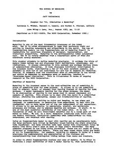
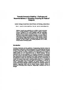
The meteorological situation on 28 May 2001 over Canada was characterized by a strong 500-mb ridge with its western edge extending from about 45◦ N to 60◦ N along ◦ about 115 W (Fig. 1). Southerly winds were present along the ridge at all levels. The low level winds transported warm and moist airmasses towards the Chisholm area inducing unstable atmospheric conditions (Fig. 2). 6047
ACPD 6, 6041–6080, 2006
Modeling pyro-convection J. Trentmann et al.
Title Page Abstract
Introduction
Conclusions
References
Tables
Figures
J
I
J
I
Back
Close
Full Screen / Esc
Printer-friendly Version Interactive Discussion
EGU
5
10
15
20
25
West of the Chisholm area a local low pressure area formed with an associated trough and cold front that moved towards the fire area (ASRD, 2001). Based on radar 1 and satellite observations (Rosenfeld et al., 2006) , a first convective line of isolated cumulonimbus, associated with the upper trough, reached the fire plume at 20:30 UTC (=14:30 MDT). Strong south-easterly surface wind prevailed after the passage of this ◦ first convective line. The maximum surface temperature reached 28 C with a minimum relative humidity of 25% indicating high fire risk (ASRD, 2001). As a result of the unstable airmass behind the first line of Cb, a second line of intense convection approached the fire area from southerly directions at about 23:00 UTC (=17:00 MDT). This convective line was more intense with maximum altitudes of radar reflectivity of about 10 km and widespread thunderstorm activity. A peak wind gust, influenced by downdrafts of the passing thunderstorm at the surface, of 92 km h−1 was measured at 00:00 UTC (ASRD, 2001). During the passage of the first convective line, the fire-induced convection started to veer, but did not intensify. The fire-induced convection was substantially intensified between 23:30 UTC and 02:30 UTC, when the second convective line approached 1 the fire (Rosenfeld et al., 2006) . Two distinctive intense pyroCbs (blow-ups) were observed in this time frame. The first occurred between 23:30 UTC and 00:30 UTC with maximum echotop heights measured by the radar of about 12 km. The second blow-up occurred between 01:20 UTC and 02:30 UTC with the arrival of the second line of convection at the fire location. Radar observations yield maximum heights for this pyro-convection between 13 km and 14 km. Satellite observations at 02:00 UTC on 29 May 2001 show a well developed convective cloud anvil covering an area of about 50 km×100 km (Rosenfeld et al., 2006)1 . An overshooting region slightly north of the fire on top of the anvil and gravity wave-like structures in the anvil are also visible. Other features of this pyro-convection include an anomalously high number of positive 1 lightning strikes (Rosenfeld et al., 2006) . In the present work, we focus on the second of this pair of intense pyro-convection events. With the help of GOES-8 satellite observations, the transport of the fire smoke in 6048
ACPD 6, 6041–6080, 2006
Modeling pyro-convection J. Trentmann et al.
Title Page Abstract
Introduction
Conclusions
References
Tables
Figures
J
I
J
I
Back
Close
Full Screen / Esc
Printer-friendly Version Interactive Discussion
EGU
5
10
15
20
25
the upper troposphere/lower stratosphere was traced (Fromm and Servranckx, 2003). It was transported by the upper level wind fields towards the north and, at about ◦ 15:00 UTC on 29 May 2001, turned eastward, north of 60 N. On 29 May 2001, 18:40 UTC, the Moderate Resolution Imaging Spectroradiometer (MODIS) and the Multi-angle Imaging SpectroRadiometer (MISR), both aboard the TERRA satellite, observed the smoke plume about 1200 km north of Chisholm. Using the information from MISR’s different viewing angles, the maximum height of the smoke layer was determined to be about 13 km, i.e, well in the stratosphere (http://eosweb.larc.nasa.gov/ HPDOCS/misr/misr html/chisholm forest fire.html). Figure 3 presents measurements taken from a radiosonde launched near Edmonton, Alberta (WMO Station Identifier 71119; 53.55◦ N, 114.10◦ W) on 29 May 2001 at 00:00 UTC (available at http://raob.fsl.noaa.gov/). These measurements, taken approx. 150 km south of the Chisholm fire, are representative of the conditions before the second line of convection has reached Chisholm. While the atmospheric boundary layer −1 was not particularly moist (absolute humidity qv =6 g kg ), the middle troposphere above 700 hPa (corresponding to 3000 m above sea level (asl)) was almost saturated. Below 700 hPa the temperature approximately followed a dry adiabatic decrease with altitude, above 700 hPa the lapse rate was slightly larger than the moist-adiabatic lapse rate. −1 With its rather low convective available potential energy (CAPE) of 131 J kg , this profile does not indicate the potential for significant convection, whereas the value for the convective inhibition (CIN) of 26 J kg−1 suggests easy initiation of convection. The lifting condensation level (LCL), the level of free convection (LFC), and the level of neutral buoyancy (LNB) of the background profile are located at 3250 m, 3620 m, and 7410 m respectively. The 0◦ C-level is at about 3400 m, i.e., close to the LCL. Based on ECMWF analysis data, the dynamical tropopause (PV>2 PVU) was located at a potential temperature of θ=332 K, corresponding to an altitude of z=11.2 km and a pressure of p=225 hPa.
ACPD 6, 6041–6080, 2006
Modeling pyro-convection J. Trentmann et al.
Title Page Abstract
Introduction
Conclusions
References
Tables
Figures
J
I
J
I
Back
Close
Full Screen / Esc
Printer-friendly Version Interactive Discussion
EGU 6049
3 Model description
5
10
15
20
25
The non-hydrostatic active tracer high resolution atmospheric model (ATHAM) (Oberhuber et al., 1998; Herzog et al., 2003) is used to simulate the pyro-convection induced by the Chisholm fire. ATHAM was originally designed and applied to simulate eruptive volcanic plumes (Graf et al., 1999). It was used to investigate the particle aggregation in an explosive volcanic eruption (Textor et al., 2006b), the impact of latent heat release and environmental conditions on the volcanic plume rise (Herzog et al., 1998; Graf et al., 1999), and the stratospheric injection of trace gases by explosive volcanic eruptions (Textor et al., 2003). It was also employed to simulate the transport of fire emissions (Trentmann et al., 2002) and the chemical processes leading to photochemical production of tropospheric ozone (Trentmann et al., 2003a). And, results obtained from ATHAM simulations were used to investigate three-dimensional radiative effects in a smoke plume (Trentmann et al., 2003b). ATHAM is formulated with a modular structure that allows the inclusion of independent modules. Existing modules treat the dynamics, turbulence, tracer transport, cloud microphysics, gas scavenging, radiation, emissions, and chemistry. In the present investigation, only the dynamics, transport, turbulence, and cloud microphysics modules of ATHAM are used. The dynamics part solves the Navier-Stokes equation for a gasparticle mixture including the transport of active tracers (Oberhuber et al., 1998). Active tracers can occur in any concentrations. They modify the density and heat capacity of the grid box average quantities, and can have a strong impact on the dynamics of the system. In the present study, the aerosol particles and all hydrometeor classes are considered as active tracers. The turbulence scheme distinguishes between horizontal and vertical turbulence exchange processes (Herzog et al., 2003). It is based on a set of three coupled prognostic equations for the horizontal and vertical turbulent kinetic energy and the turbulent length scale. Cloud microphysical processes are simulated using a two-moment scheme that predicts the numbers and mass mixing ratios of four classes of hydrometeors (cloud water, 6050
ACPD 6, 6041–6080, 2006
Modeling pyro-convection J. Trentmann et al.
Title Page Abstract
Introduction
Conclusions
References
Tables
Figures
J
I
J
I
Back
Close
Full Screen / Esc
Printer-friendly Version Interactive Discussion
EGU
5
10
15
20
25
cloud ice, rain, graupel) and water vapour (Textor et al., 2006a). Due to the high abun−3 dance of smoke aerosol (>80 000 cm ) in pyro-convection only a small fraction of it becomes activated. As cloud (ice) particle nucleation is not explicitly calculated, for this study, we assume that 5% of the smoke aerosol particles act as cloud (or ice) condensation nuclei. This number is an upper limit of estimates based on box model simulations for a comparable situation (large aerosol number concentrations and updraft velocities) with an explicit description of condensation (Martin Simmel, pers. comm., 2003; Simmel and Wurzler, 2006). Despite the very high droplet number concentrations obtained with this assumption, it was found that the microphysically induced effect of the fire aerosols on dynamics is rather small (Luderer et al., 2006a). This justifies the simplified approach used here. The simplification limits, however, the use of ATHAM for detailed microphysical studies on the aerosol effect on the evolution and the precipitation efficiency of pyro-convection. Work is in progress to implement a more complex cloud microphysical scheme that includes the activation of aerosol (Khain et al., 2004). ATHAM is three-dimensionally formulated with an implicit time-stepping scheme. The solution of the Navier-Stokes equation is computed on a cartesian grid. A grid stretching allows the use of a higher spatial resolution in predefined regions of the model domain than at the model boundaries. A mass-conservative form of the transport equation is employed for all tracers. The focus of this study is the detailed description of the impact of fire emissions on the atmosphere in the vicinity of the fire on a horizontal scale of about 100 km. The fluxes from the fire to the atmosphere are prescribed, and therefore not modified by the meteorological conditions, e.g., the wind speed and direction. The reduced requirements for computer resources allow a detailed description of the atmospheric processes related to fire-induced convection. Other numerical models that include the interaction between the atmosphere and fire result in a more realistic fire evolution and small scale features of the atmospheric fields (Clark et al., 2004; Linn et al., 2005). However, they do not consider all relevant processes (e.g., cloud microphysics) to describe the evolution of deep pyro-convection on the timescale considered here. 6051
ACPD 6, 6041–6080, 2006
Modeling pyro-convection J. Trentmann et al.
Title Page Abstract
Introduction
Conclusions
References
Tables
Figures
J
I
J
I
Back
Close
Full Screen / Esc
Printer-friendly Version Interactive Discussion
EGU
4 Model setup and initialization
5
10
15
20
For the present study, ATHAM is initialized to realistically represent the conditions of the convective event induced by the Chisholm fire. The model domain was set to 84 km×65 km×26 km with 110×85×100 grid boxes in the x-, y-, and z-directions, respectively. The minimum horizontal grid box size was set to 500 m and 100 m in the x- and y-directions, respectively. Due to the stretched grid, the size of the grid boxes increases towards the borders of the model domain. The vertical grid spacing at the surface and the tropopause was set to 50 m and 150 m, respectively. Outside these regions, slightly larger vertical grid spacings were used. The lowest vertical model level is located at 766 m a.s.l., corresponding to the lowest elevation available in the radiosonde data used for the model initialization, and close to the elevation of Chisholm of about 600 m (ASRD, 2001). Throughout the manuscript, model elevations are given in m asl. An adaptive dynamical timestep between 1 sec and 3 sec was used, determined online by the Courant-Friedrichs-Lewy (CFL) criterion (CFL≤0.8). The model simulation was conducted for 40 min. The model domain was initialized horizontally homogeneously with measurements obtained from the radiosonde presented in Sect. 2.2, Fig. 3. Open lateral boundaries were used for the model simulations. The horizontal means of the directional wind speed (u, v) and of the specific humidity (qv ) were nudged towards the initial profile at the lateral boundaries. 4.1 Representation of the fire emissions
25
The fire is represented in the model by time-constant fluxes of sensible heat, water vapor, and aerosol mass into the lowest vertical model layer. The fire front was approximately linear and extended from south-south-east to north-north-west at an angle of approximately 165◦ to North. Note that the x-axis of the model coordinate frame was aligned with the fire front, such that the x-direction of the model domain is at an angle of 165◦ to North. 6052
ACPD 6, 6041–6080, 2006
Modeling pyro-convection J. Trentmann et al.
Title Page Abstract
Introduction
Conclusions
References
Tables
Figures
J
I
J
I
Back
Close
Full Screen / Esc
Printer-friendly Version Interactive Discussion
EGU
5
10
15
20
25
The actual length of the fire front was about 25 km. Due to computational constraints, however, we only accounted for the southern 15 km of the fire front, which passed through densely forested area. The width of the fire front was set to 500 m. The −2 energy release from the fire was calculated based on a fuel loading of 9.0 kg m and −1 a value of 18 700 kJ kg for the heat of combustion. Based on the comparably high fuel load in the southern part of the fire front, we choose a higher-than-average fuel loading in the simulations. With the observed rate of spread of the fire front of 1.5 m s−1 , the frontal intensity (Byram, 1959; Lavoue´ et al., 2000) of the simulated fire is about 250 000 kW m−1 . There is significant uncertainty in the literature on how much of the energy, released by combustion, contributes to local heating of the atmosphere (sensible heat flux) and is available for convection, and how much of the energy is lost due to radiative processes. Commonly found estimates for the radiative energy are between nearly zero percent (Wooster, 2002; Wooster et al., 2005) and 50% (McCarter and Broido, 1965; Packham, 1969). These estimates are based on laboratory studies or small scale fires and their application to large scale crown fires resulting in pyroCb convection remains highly uncertain. For the present model simulations, we assume that all energy released in the combustion process becomes available for convection. This assumption is consistent with the coupled fire-atmosphere model of Clark et al. (1996). In the companion paper, we present the sensitivity of the model results to assumptions of the release of sensible heat (Luderer et al., 2006a). A small part of the energy released by the combustion of fuel is used to evaporate the fuel moisture. In the present study, a fuel moisture content of 40% was assumed (see Sect. 2.1), which takes up about 5% of the total energy released by the combustion. Additional water vapor is released directly from the combustion process itself. Assuming complete combustion, 1 kg of fuel yields about 0.5 kg of combustion water vapor −2 (Byram, 1959). In our simulations, about 8 kg m water vapor was released, with the main contribution (about 55%) coming from combustion moisture, leading to a total re8 lease of 4.7×10 kg H2 O. The particulate emissions from the fire were calculated using 6053
ACPD 6, 6041–6080, 2006
Modeling pyro-convection J. Trentmann et al.
Title Page Abstract
Introduction
Conclusions
References
Tables
Figures
J
I
J
I
Back
Close
Full Screen / Esc
Printer-friendly Version Interactive Discussion
EGU
5
10
the emission factor of 17.6 g kg−1 from Andreae and Merlet (2001). No detailed information on the wind direction at the location of the fire front at the time of the blow-up is available. Due to the complex meteorological situation (i.e., the approaching line of convection) it is likely that the local wind speed and wind direction were irregular and subject to rapid change. These effects cannot be represented with the model approach of this study. Therefore, we adopted the wind profile measured by the Edmonton radiosonde. Its surface wind direction is at an angle of about 30◦ to the fire front. In the upper atmospheric levels, the ambient wind direction is parallel to the fire front. The angle between the wind field and the fire front has some impact on the average time that individual parcels are exposed to the fire.
ACPD 6, 6041–6080, 2006
Modeling pyro-convection J. Trentmann et al.
Title Page
5 Model results
15
20
25
In the following, results from the model simulations are presented. First, we will show the overall structure of the simulated pyroCb, and then investigate some dynamical features in more detail in Sect. 5.1. −3 Figure 4 shows the simulated extent of the 150 µg m -isosurface of the aerosol mass distribution after 40 min of simulation time. The color coding represents the potential temperature. The assumed linear shape of the fire front is clearly visible as the origin of the convection and the source of the aerosol particles. The maximal height of the aerosol plume of about 12.5 km is reached above the fire. The plume reaches well into the stratosphere as can be inferred from the values of the potential temperatures above 332 K. Large areas of the plume have a potential temperature of more than 340 K. Downwind of the overshooting region, a relatively warm area develops in the anvil region with potential temperatures above 350 K. This is consistent with the warm core of the Chisholm pyroCb observed by satellite (Fromm and Servranckx, 1 2003; Rosenfeld et al., 2006 ). A more detailed investigation of the plume top structures including an evaluation of the model results with satellite observations will be 6054
Abstract
Introduction
Conclusions
References
Tables
Figures
J
I
J
I
Back
Close
Full Screen / Esc
Printer-friendly Version Interactive Discussion
EGU
5
10
15
20
25
presented in Luderer et al. (2006b)2 . −1 Figure 5 presents the spatial distribution of the 0.4 g kg -isosurfaces of the four hydrometeor classes (cloud water, rain, cloud ice, and graupel) at the end of the simulation. Graupel is the main contributor to the hydrometeor mass in the simulated pyroCb. It is interesting to note that cloud ice is dominant in the upper part of the cloud due to the sedimentation of the large hydrometeors. The size of the hydrometeors remains comparably small due to the high concentration of smoke aerosol acting as CCN and the large updraft velocities (Luderer et al., 2006a). Figure 6 shows the temporal evolution of the spatially integrated mass of the four hydrometeor classes in the model domain. The first cloud water condenses after about 4 min of simulation time at an elevation of about 4.2 km. The enhanced temperature in the plume leads to delayed condensation compared to the LCL derived from the initial background profile (3.25 km). After about 10 min, the graupel class becomes the dominant class in the pyro-cloud. Cloud ice has the second largest contribution to the total hydrometeor mass followed by cloud and rain water. Figure 7 shows the horizontally integrated aerosol mass as function of altitude and potential temperature after 40 min of simulation time. The main outflow height (defined as the height of the maximum of the vertically integrated aerosol distribution) and the maximum penetration height (defined as the height below which 99 % of the aerosol mass is located) are 10.6 km and 12.1 km, respectively. The outflow height is substantially higher than the level of neutral buoyancy calculated based on the sounding (7410 m, Sect. 2.2), due to the significant emissions of sensible heat from the fire. A substantial amount of aerosol mass is located at stratospheric potential temperature levels (θ>332 K). Overall, 710 t aerosol mass was deposited into the stratosphere, corresponding to about 8% of the total emitted aerosol mass. Whether the smoke aerosol will remain in the stratosphere after the pyro-convection has deceased can not be eval-
ACPD 6, 6041–6080, 2006
Modeling pyro-convection J. Trentmann et al.
Title Page Abstract
Introduction
Conclusions
References
Tables
Figures
J
I
J
I
Back
Close
Full Screen / Esc
Printer-friendly Version Interactive Discussion
2
¨ Luderer, G., Trentmann, J., Hungershofer K., et al.: The role of small scale processes in troposphere-stratosphere transport by pyro-convection, Atmos. Phys. Chem. Discuss., in preparation, 2006.
6055
EGU
5
10
15
20
25
uated with the present model setup that only allows model simulations for about 40 min. The present simulation, however, does show that pyro-convection can be sufficiently intense to transport smoke aerosol across the tropopause and into the stratosphere. To estimate the contribution of the latent heat release via condensation and freezing to the release of sensible heat by the fire, we calculate the total heat of condensation and freezing based on the total mass of hydrometeors in the model domain (8.22×10⁹ kg frozen hydrometeors, 1.4×10⁹ kg liquid hydrometeors) to be 26.8×10⁹ MJ. This value can be considered an lower estimate of the total energy release by condensation/freezing, since deposition of hydrometeors is neglected in this simplified estimate. This number can be compared to the total amount of sensible heat emitted from the fire during the simulation which sums up to 9×10⁹ MJ. This estimate yields that about 25% of the total energy results from direct emission of sensible heat from the fire, while the dominant part of the energy budget can be attributed to the release of latent heat during condensation and freezing. The latent heat released from the fire contributes less than 5% to the total energy released from condensation and freezing (see Sect. 4.1). A similar estimate is obtained, when we consider an individual parcel in the upper −3 part of the plume with an average aerosol mass concentration of 3000 µg m and a −1 hydrometeor concentration of about 5 g kg . Based on the emission ratios for sensible heat, water vapor, and particles, this parcel gained about 6 K of sensible heat and 0.3 g kg−1 H2 O from the fire. The hydrometeor concentration corresponds to a release of latent heat from condensation of about 12 K. This parcel-based estimate yields a slightly larger contribution of the sensible heat flux from the fire to the parcel energy than the previous estimate based on the energy budget for the whole pyroCb. Both estimates highlight the importance of the availability of ambient moisture for the evolution of the pyro-convection. In the following, some aspects of the evolution of the pyro-convection are discussed.
ACPD 6, 6041–6080, 2006
Modeling pyro-convection J. Trentmann et al.
Title Page Abstract
Introduction
Conclusions
References
Tables
Figures
J
I
J
I
Back
Close
Full Screen / Esc
Printer-friendly Version Interactive Discussion
EGU 6056
5.1 Convection dynamics
5
10
15
20
25
After the onset of the heat flux from the fire, convection immediately develops in the model simulations due to the positive temperature anomaly of the air in the lowest model layer above the fire. Figure 8 presents streamlines of the horizontal wind and the vertical wind velocity at 1000 m a.s.l. (i.e., about 200 m a.g.l.) after 40 min of simulation. The fire clearly has a strong impact on the ambient wind field. The emission of sensible heat leads to high updraft velocities of up to 20 m s−1 . The updraft results in the formation of a convergence of the horizontal wind. The simulated updraft velocities at the surface are signifcantly higher than those expected for regular convection. In the case of pyroconvection, the updraft initiates the convergence of the low-level horizontal wind, while regular convection often starts from low level wind convergence. This wind modification is expected to significantly impact the evolution of the fire itself as has been shown in coupled atmosphere-fire simulations (Clark et al., 2004; Coen, 2005). Since the focus of this work is the investigation of the vertical transport of fire emissions, this feedback mechanism is not included here and the shape of the fire and the fire emissions are kept constant throughout the simulation. Figure 9 shows the temporal evolution of some quantities used to characterize the dynamical evolution of the convection. Shown are the maximum vertical velocity, wmax , the aerosol-mass-weighted mean vertical velocity, w, and the integrated buoyancy, IB. w is defined by Z 1 w=R w ca dV. (1) ca dV The highest vertical velocities and aerosol loadings are located directly above the fire. To investigate processes in the pyroCb and compare different model simulations, this region, which is dominated by the fire emissions, needs to be excluded from the calculations. Therefore, we limit the calculation of the mean velocity to grid boxes with a hydrometeor content of more than 0.05 g kg−1 . By including only grid boxes with a 6057
ACPD 6, 6041–6080, 2006
Modeling pyro-convection J. Trentmann et al.
Title Page Abstract
Introduction
Conclusions
References
Tables
Figures
J
I
J
I
Back
Close
Full Screen / Esc
Printer-friendly Version Interactive Discussion
EGU
vertical velocity w ≥ 5 m s−1 we limit this estimate to strong updrafts. ca is the aerosol mass concentration. IB is defined by IB =
6, 6041–6080, 2006
ZZLNB
b(z) dz,
(2)
Z0
5
10
15
20
25
ACPD
where the integration is performed from ground level z0 to the level of neutral buoyancy zLNB with b(zLNB )=0. b(z) is the average buoyancy in the updraft calculated using the vertical aerosol flux as the weight function (see Luderer et al., 2006a for a full description of these quantities). After about 20 min of simulation time, all quantities shown in Fig. 9 remain relatively constant, indicating that at least the dynamics of the updraft region reaches a steady state. The maximum updraft velocity still oscillates at the end of the simulation indicating the complex dynamical coupling of the sensible heat flux from the fire with the atmospheric flow. At the end of the simulation, the maximum updraft, wmax , the mean updraft velocity, w, and the integrated buoyancy, IB, are 38 m s−1 , 17.5 m s−1 , and 1800 J kg−1 , respectively. The difference between the CAPE of the ambient profile −1 (131 J kg ) and the calculated IB can mainly be attributed to the emissions of sensible heat from the fire. Figure 10 shows a cross section of the vertical velocity along the y-axis after 40 min. The maximum vertical velocity is reached right above the fire, below the 2000 m level. −1 At the tropopause, a region with downward vertical motions of about 6 m s is simulated downwind of the fire. One has to note, that the interpretation of individual cross sections is complex, especially due to the asymmetric ambient flow. In contrast to simulations of mid-latitude convection, the maximum vertical velocity is reached at lower levels in the case of fire-induced convection (between 1 km and 3 km compared to about 9 km in Wang, 2003 and Mullendore et al., 2005). This is explained by the significant acceleration by the heat flux from the fire. A second local maximum of the updraft velocity can be found at about 8 km (Fig. 10), which corresponds to 6058
Modeling pyro-convection J. Trentmann et al.
Title Page Abstract
Introduction
Conclusions
References
Tables
Figures
J
I
J
I
Back
Close
Full Screen / Esc
Printer-friendly Version Interactive Discussion
EGU
5
10
15
20
25
the maximum of the updraft velocity in simulations of regular mid-latitude convection due to the release of latent heat. The different vertical profiles in the updraft velocity, in particular at cloud base, between regular mid-latitude convection and fire-induced convection potentially lead to differences in the cloud microphysical evolution in addition to the high number of smoke particles acting as CCN. Shown in Fig. 11 is the simulated temperature anomaly after 40 min along the cross section at y=0 km. The fire-released heat flux induces a temperature anomaly in the lower 2 km of the rising plume with maximum values in the layer above the fire. About 1 km above the fire, the temperature anomaly has decreased to values smaller than 20 K, at about 3 km it is only about 8 K. In the upper part of the plume, a dipole-like structure of the temperature anomaly can be seen. This is associated with a gravity wave at the tropopause and will be presented in detail in Luderer et al. (2006b)2 . For photochemical reactions occurring in the smoke plume, this temperature enhancement can be regarded as small and can be neglected in photochemical models of young biomass burning plumes (Mason et al., 2001; Trentmann et al., 2005). The modification of the ambient temperature is, however, significant for the condensation of water vapor and the level of cloud base (see Sect. 5). The increased temperature leads to a delayed onset of condensation and a higher cloud base, thereby counteracting the effect of the water vapor emissions from the fire on the cloud base. The contribution of the water vapor emitted by the fire to the total water vapor is shown in Fig. 12. The emitted water dominates the atmospheric water vapor concentration right above the fire, but due to mixing of the plume with environmental air masses, the contribution of the water vapor from the fire rapidly decreases at higher altitude. Above about 4000 m, the contribution of water vapor from the fire is less than 10% of the total water vapor available in the plume. This analysis and a sensitivity study presented in Luderer et al. (2006a) shows that in the case of the Chisholm fire, the water vapor emitted from the fire does not have a significant impact on the evolution of the cloud and atmospheric dynamics. This result is consistent with the findings from previous model studies (Penner et al., 1986; Small and Heikes, 1988). 6059
ACPD 6, 6041–6080, 2006
Modeling pyro-convection J. Trentmann et al.
Title Page Abstract
Introduction
Conclusions
References
Tables
Figures
J
I
J
I
Back
Close
Full Screen / Esc
Printer-friendly Version Interactive Discussion
EGU
5
10
15
20
Entrainment of ambient air into the plume significantly reduces the contribution of the water vapor from the fire to the total water vapor in the plume. To investigate the amount of mixing, six tracers were initialized within six separate layers of identical mass. The lower boundaries of the layers are the surface, 2.25 km, 4 km, 6.1 km, 8.9 km, and 12.9 km. The relative contribution of the different tracer masses in the smoke plume after 40 min of simulation is shown in Fig. 13. The air masses in the main outflow of the plume mainly originate from the two lower levels (Tracer I and Tracer II), each contributing about 30% to the total air mass in the plume. The significant contribution of the mid-level Tracer II indicates significant entrainment of ambient airmasses into the plume between 2.25 km and 4 km. Additional contributions to the air in the outflow come from Tracers III, IV, and Tracer V. These findings are consistent with the modeling results from Mullendore et al. (2005), who also found significant entrainment of ambient air from the middle troposphere into the updraft and the outflow of convective systems. The significant contribution of mid-level air masses in the plume point to the potential importance of the background conditions, e.g. the humidity, for the evolution of the pyro-convection. The high amounts of entrainment also limit the use of the CAPE concept, which usually neglects entrainment, to characterize pyro-convection events. The non-negligible contributions of tracers V and VI in the smoke plume especially at elevations above 12 km give evidence for the occurrence of mixing processes and downward transport of stratospheric air at the tropopause level. 6 Conclusions and outlook
25
ACPD 6, 6041–6080, 2006
Modeling pyro-convection J. Trentmann et al.
Title Page Abstract
Introduction
Conclusions
References
Tables
Figures
J
I
J
I
Back
Close
Full Screen / Esc
We presented three-dimensional model simulations of the pyro-convection associated with the Chisholm fire in Alberta, May 2001. During its most intense phase, the Chisholm fire burned 50 000 ha of forested land within a few hours, resulting in the formation of an intense fire-induced cumulonimbus (pyroCb). Using fire emissions based on available estimates for the amount of fuel burned and measurements obtained by a radiosonde at a distance of about 100 km, the model is able to realistically simulate 6060
Printer-friendly Version Interactive Discussion
EGU
5
10
15
20
25
30
the formation and the evolution of the pyro-convection. In particular, the maximum penetration height of the pyro-convection (about 12.1 km) compares well with radar observations, and the injection of smoke aerosol into the stratosphere is simulated in accordance with satellite observations. The character of the pyro-convection is different from regular mid-latitude convection. Mainly owing to the sensible heat emissions from the fire, the main outflow is significantly higher than the level of neutral buoyancy of the background atmosphere. More modeling studies of this kind are required to fully understand the nature of pyro-convection. The intensity of pyro-convection determines the injection height of fire emissions, which is important for their atmospheric lifetime and impact. Injection of smoke from fires at high altitude into the atmosphere increases its lifetime compared to injection in the boundary layer and may result in hemispheric and seasonal effects of the smoke from a single pyroCb event on the atmosphere. PyroCb studies of the kind presented here, using different scenarios for the fire emissions and atmospheric conditions, will lead to a more realistic representation of fire emissions in larger scale models. Studies such as the present one also make it possible to take into account the smallscale processes in pyro-clouds that lead to a modification of the primary fire emissions (e.g., photochemistry, scavenging of soluble gases and particles). The investigation of these and other processes (e.g., aerosol-cloud interaction) using a combination of model simulations and field observations will lead to an improved representation of fire emissions in larger scale models and will also advance our understanding of these fundamental processes in regular convective clouds. Acknowledgements. J. Trentmann thanks the Alexander von Humboldt-foundation for support through a Feodor-Lynen fellowship. G. Luderer was supported by an International Max Planck Research School fellowship. Part of this research was supported by the German Ministry for Education and Research (BMBF) under grant 07 ATF 46 (EFEU), by the Helmholtz Association (Virtual Institute COSI-TRACKS), and by the German Max Planck Society. DWD and ECMWF are acknowledged for providing access to ECMWF Data. J. Trentmann is indebted to the late P. V. Hobbs for his advice, support, und the opportunity to start this project while part being of the Cloud and Aerosol Research Group (CARG) at the University of Washington. Discus-
6061
ACPD 6, 6041–6080, 2006
Modeling pyro-convection J. Trentmann et al.
Title Page Abstract
Introduction
Conclusions
References
Tables
Figures
J
I
J
I
Back
Close
Full Screen / Esc
Printer-friendly Version Interactive Discussion
EGU
sions with H. Wernli, A. Khain, M. Simmel, A. Rangno, D. Rosenfeld, D. Hegg, G. Mullendore, M. Stoelinga, E. Jensen, D. Diner, and M. Watton are highly appreciated.
ACPD 6, 6041–6080, 2006
References
5
10
15
20
25
Andreae, M. O. and Merlet, P.: Emission of trace gases and aerosols from biomass burning, Global Biogeochem. Cycles, 15, 955–966, 2001. 6043, 6054 ASRD: Final Documentation Report – Chisholm Fire (LWF-063), Forest Protection Division, ISBN 0-7785-1841-8, Tech. rep., Alberta Sustainable Resource Development, 2001. 6046, 6047, 6048, 6052 Banta, R. M., Olivier, L. D., Holloway, E. T., Kropfli, R. A., Bartram, B. W., Cupp, R. E., and Post, M. J.: Smoke.Column Observations from Two Forest Fires Using Doppler Lidar and Doppler Radar, J. Appl. Meteorol., 31, 1328–1349, 1992. 6044 Byram, G. M.: Combustion of forest fuels, in: Forest Fire Control and Use, edited by: Davis, K. P., McGraw-Hill, New York, 1959. 6053 Chuang, C. C., Penner, J. E., and Edwards, L. L.: Nucleation Scavenging of Smoke Particles and Simulated Drop Size Distributions over Large Biomass Fires, J. Atmos. Sci., 49, 1264– 1275, 1992. 6045 Clark, T. L., Jenkins, M. A., Coen, J., and Packham, D.: A Coupled Atmosphere-Fire Model: Convective Feedback on Fire-Line Dynamics, J. Appl. Meteorol., 35, 875–901, 1996. 6045, 6053 Clark, T. L., Coen, J., and Latham, D.: Description of a coupled atmosphere-fire model, Int. J. Wildland Fire, 13, 49–63, 2004. 6045, 6051, 6057 Coen, J.: Simulation of the Big Elk Fire using coupled atmosphere-fire modeling, Int. J. Wildland Fire, 14, 49–59, 2005. 6057 Crutzen, P. J. and Andreae, M. O.: Biomass Burning in the Tropics: Impact on Atmospheric Chemistry and Biogeochemical Cycles, Science, 250, 1669–1678, 1990. 6043 Cunningham, P., Goodrick, S. L., Hussaini, M. Y., and Linn, R. R.: Coherent vortical structures in numerical simulations of buoyant plumes from wildland fires, Int. J. Wildland Fire, 14, 61–75, 2005. 6045 Damoah, R., Spichtinger, N., Servranckx, R., Fromm, M., Eloranta, E. W., Razenkov, I. A.,
Modeling pyro-convection J. Trentmann et al.
Title Page Abstract
Introduction
Conclusions
References
Tables
Figures
J
I
J
I
Back
Close
Full Screen / Esc
Printer-friendly Version Interactive Discussion
EGU 6062
5
10
15
20
25
30
James, P., Shulski, M., Foster, C., and Stohl, A.: A case study of pyro-convection using transport model and remote sensing data, Atmos. Chem. Phys., 6, 173–185, 2006. 6043 FIRESCAN Science Team: Fire in Ecosystems of Boreal Eurasia: The Bor Forest Island Fire Experiment, Fire Research Campaign Asia-North (FIRESCAN), in: Biomass Burning and Global Change, edited by: Levine, J. S., 848–873, MIT Press, Cambridge, Mass., 1996. 6044 Fromm, M., Alfred, J., Hoppel, K., Hornstein, J., Bevilacqua, R., Shettle, E., Servranckx, R., Li, Z., and Stocks, B.: Observations of boreal forest fire smoke in the stratosphere by POAM III, SAGE II, and lidar in 1998, Geophys. Res. Lett., 27, 1407–1410, 2000. 6043, 6044 Fromm, M., Bevilacqua, R., Servranckx, R., Rosen, J., Thayer, J. P., Herman, J., and Larko, D.: Pyro-cumulonimbus injection of smoke to the stratosphere: Observations and impact of a super blowup in northwestern Canada on 3–4 August 1998, J. Geophys. Res., 110, D08205, doi:10.1029/2004JD005350, 2005. 6043, 6044 Fromm, M., Tupper, A., Rosenfeld, D., Servranckx, R., and McRae, R.: Violent pyro-convective storm devastates Australia’s capital and pollutes the stratosphere, Geophys. Res. Lett., 33, L05815, doi:10.1029/2005GL025161, 2006. 6044 Fromm, M. D. and Servranckx, R.: Transport of forest fire smoke above the tropopause by supercell convection, Geophys. Res. Lett., 30, 1542, doi:10.1029/2002GL016820, 2003. 6044, 6045, 6046, 6049, 6054 ´ S. and Hegg, D. A.: Comparison of Columnar Aerosol Optical Properties Measured by Gasso, the MODIS Airborne Simulator with In Situ Measurements: A Case Study, Remote Sens. Environ., 66, 138–152, 1998. 6044 Gostintesev, Y. A., Kopylov, N. P., Ryzhov, A. M., and Khazanov, I. R.: Numerical modeling of convective flows above large fires at various atmospheric conditions, Combust., Expl., Shock Waves, 27, 656–662, 1991. 6045 Graf, H.-F., Herzog, M., Oberhuber, J. M., and Textor, C.: The effect of environmental conditions on volcanic plume rise, J. Geophys. Res., 104, 24 309–24 320, 1999. 6050 Herzog, M., Graf, H.-F., Textor, C., and Oberhuber, J. M.: The effect of phase changes of water on the development of volcanic plumes, J. Volcanol. Geotherm. Res, 87, 55–74, 1998. 6050 Herzog, M., Oberhuber, J. M., and Graf, H.-F.: A Prognostic Turbulence Scheme for the Nonhydrostatic Plume Model ATHAM, J. Atmos. Sci., 60, 2783–2796, 2003. 6050 Hobbs, P. V., Reid, J. S., Herring, J. A., Nance, J. D., Weiss, R. E., Ross, J. L., Hegg, D. A., Ottmar, R. D., and Liousse, C.: Particle and Trace-Gas Measurements in the Smoke from
6063
ACPD 6, 6041–6080, 2006
Modeling pyro-convection J. Trentmann et al.
Title Page Abstract
Introduction
Conclusions
References
Tables
Figures
J
I
J
I
Back
Close
Full Screen / Esc
Printer-friendly Version Interactive Discussion
EGU
5
10
15
20
25
30
Prescribed Burns of Forest Products in the Pacific Northwest, in: Biomass Burning and Global Change, edited by: Levine, J. S., 697–715, MIT Press, Cambridge, Mass., 1996. 6044, 6045 Hobbs, P. V., Sinha, P., Yokelson, R. J., Christian, T. J., Blake, D. R., Gao, S., Kirchstetter, T. W., Novakov, T., and Pilewskie, P.: Evolution of gases and particles from a savanna fire in South Africa, J. Geophys. Res., 108, 8485, doi:10.1029/2002JD002352, 2003. 6044 Immler, F., Engelbart, D., and Schrems, O.: Fluorescence from atmospheric aerosol detected by a lidar indicates biogenic particles in the lowermost stratosphere, Atmos. Chem. Phys., 5, 345–355, 2005. 6043 Jenkins, M. A.: Investigating the Haines Index using parcel model theory, Int. J. Wildland Fire, 13, 297–309, 2004. 6045 Jost, H.-J., Drdla, K., Stohl, A., Pfister, L., Loewenstein, M., Lopez, J. P., Hudson, P. K., Murphy, D. M., Cziczo, D. J., Fromm, M., Bui, T. P., Dean-Day, J., Gerbig, C., Mahoney, J., Richard, E. C., Spichtinger, N., Pittman, J. V., Weinstock, E. M., Wilson, J. C., and Xueref, I.: In-situ observations of mid-latitude forest fire plumes deep in the stratosphere, Geophys. Res. Lett., 31, L11101, doi:10.1029/2003GL019253, 2004. 6043 Khain, A., Pokrovsky, A., Pinsky, M., Seifert, A., and Phillips, V.: Simulation of Effects of Atmospheric Aerosols on Deep Turbulent Convective Clouds Using a Spectral Microphysics Mixed-Phase Cumulus Cloud Model. Part I: Model Description and Possible Applications, J. Atmos. Sci., 61, 2963–2982, 2004. 6051 ´ D., Liousse, C., Cachier, H., Stocks, B. J., and Goldammer, J. G.: Modeling of carbonaLavoue, ceous particles emitted by boreal and temperate wildfires at northern latitudes, J. Geophys. Res., 105, 26 871–26 890, 2000. 6045, 6053 Linn, R., Winterkamp, J., Colman, J. J., Edminster, C., and Bailey, J. D.: Modeling interactions between fire and atmosphere in discrete element fuel beds, Int. J. Wildland Fire, 14, 37–48, 2005. 6045, 6051 Livesey, N. J., Fromm, M. D., Waters, J. W., Manney, G. L., Santee, M. L., and Read, W. G.: Enhancements in lower stratopsheric CH3 CN observed by the Upper Atmosphere Research Satellite Microwave Limb Sounder following boreal forest fires, J. Geophys. Res., 109, D06308, doi:10.1029/2003JD004055, 2004. 6043 Luderer, G., Trentmann, J., Winterrath, T., Textor, C., Herzog, M., Graf, H.-F., and Andreae, M. O.: Modeling of Biomass Smoke Injection into the Lower Stratosphere (Part II): Sensitivity Studies, Atmos. Chem. Phys. Discuss., 6, 6081–6124, 2006a. 6046, 6051, 6053, 6055,
6064
ACPD 6, 6041–6080, 2006
Modeling pyro-convection J. Trentmann et al.
Title Page Abstract
Introduction
Conclusions
References
Tables
Figures
J
I
J
I
Back
Close
Full Screen / Esc
Printer-friendly Version Interactive Discussion
EGU
5
10
15
20
25
30
6058, 6059 Manis, P. C.: Cloud heights and stratospheric injections resulting from a thermonuclear war, Atmos. Environ., 19, 1245–1255, 1985. 6045 Mason, S. A., Field, R. F., Yokelson, R. J., Kochivar, M. A., Tinsley, M. R., Ward, D. E., and Hao, W. M.: Complex effects arising in smoke plume simulations due to inclusion of direct emissions of oxygenated organic species from biomass combustion, J. Geophys. Res., 106, 12 527–12 539, 2001. 6059 McCarter, R. J. and Broido, A.: Radiative and convective energy from wood crib fires, Pyrodynamics, 2, 65–85, 1965. 6053 Mitchell, R. M., O’Brien, D. M., and Campbell, S. K.: Characteristics and radiative impact of the aerosol generated by the Canberra firestorm of January 2003, J. Geophys. Res., 111, D02204, doi:10.1029/2005JD006304, 2006. 6044 Morton, B. R., Taylor, S. G., and Turner, J. S.: Turbulent gravitational convection from maintained and instantaneous sources, Proc. R. Soc. Ser. A, 234, 1–23, 1956. 6045 Mullendore, G. L., Durran, D. R., and Holton, J. R.: Cross-tropopause tracer transport in midlatitude convection, J. Geophys. Res., 110, D06113, doi:10.1029/2004JD005059, 2005. 6058, 6060 Nedelec, P., Thouret, V., Brioude, J., Sauvage, B., Cammas, J.-P., and Stohl, A.: Extreme CO concentrations in the upper troposphere over northeast Asia in June 2003 from the in situ MOZAIC aircraft data, Geophys. Res. Lett., 32, L14807, doi:10.1029/2005GL023141, 2005. 6043 Oberhuber, J. M., Herzog, M., Graf, H.-F., and Schwanke, K.: Volcanic plume simulation on large scales, J. Volcanol. Geotherm. Res, 87, 29–53, 1998. 6050 Packham, D. R.: Heat transfer above a small ground fire, Aust. For. Res., 5, 19–24, 1969. 6053 Penner, J. E., Haselman, Jr., L. C., and Edwards, L. L.: Smoke-Plume Distribution above LargeScale Fires: Implications for Simulations of “Nuclear Winter”, J. Climate and Appl. Meteorol., 25, 1434–1444, 1986. 6045, 6059 Penner, J. E., Bradley, M. M., Chuang, C. C., Edwards, L. L., and Radke, L. F.: A Numerical Simulation of the Aerosol-Cloud Interaction and Atmospheric Dynamics of the Hardiman Township, Ontario, Prescribed Burn, in: Global Biomass Burning: Atmospheric, Climatic, and Biospheric Implications, edited by: Levine, J. S., 420–426, MIT Press, Cambridge, Mass., 1991. 6045 Radke, L., Hegg, D., Lyons, J., Brock, C., Hobbs, P., Weiss, R., and Rasmussen, R.: Airborne
6065
ACPD 6, 6041–6080, 2006
Modeling pyro-convection J. Trentmann et al.
Title Page Abstract
Introduction
Conclusions
References
Tables
Figures
J
I
J
I
Back
Close
Full Screen / Esc
Printer-friendly Version Interactive Discussion
EGU
5
10
15
20
25
30
measurements on smoke from biomass burning, in: Aerosols and Climate, edited by: Hobbs, P. V. and McCormick, P., 411–422, A. DEEPAK Publishing, 1988. 6044 Radke, L. F., Hegg, D. A., Hobbs, P. V., Nance, J. D., Lyons, J. H., Laursen, K. K., Weiss, R. E., Riggan, P. J., and Ward, D. E.: Particulate and Trace Gas Emissions from Large Biomass Fires in North America, in: Global Biomass Burning: Atmospheric, Climatic, and Biospheric Implications, edited by: Levine, J. S., 209–224, MIT Press, Cambridge, Mass., 1991. 6044 Siebert, J., Timmis, C., Vaughan, G., and Fricke, K. H.: A strange cloud in the Artic summer stratosphere 1998 above Esrange (68◦ N), Sweden, Annales Geophysicae, 18, 505–509, 2000. 6043 Simmel, M. and Wurzler, S.: Condensation and activation in sectional cloud microphysical models, Atmos. Res., 80, 218–236, 2006. 6051 Small, R. D. and Heikes, K. E.: Early Cloud Formation by Large Area Fires, J. Appl. Meteorol., 27, 654–663, 1988. 6045, 6059 Stocks, B. J., Alexander, M. E., and Lanoville, R. A.: Overview of the International Crown Fire Modelling Experiment (ICFME), Can. J. For. Res., 34, 1543–1547, 2004. 6044 Textor, C., Graf, H.-F., Herzog, M., and Oberhuber, J. M.: Injection of gases into the stratosphere by explosive volcanic eruptions, J. Geophys. Res., 108, 4606, doi:10.1029/2002JD002987, 2003. 6050 Textor, C., Graf, H. F., Herzog, M., Oberhuber, J. M., Rose, W. I., and Ernst, G. G. J.: Volcanic particle aggregation in explosive eruption columns. Part I: Parameterization of the microphysics of hydrometeors and ash, J. Volcanol. Geotherm. Res, 150, 359–377, 2006a. 6051 Textor, C., Graf, H. F., Herzog, M., Oberhuber, J. M., Rose, W. I., and Ernst, G. G. J.: Volcanic particle aggregation in explosive eruption columns. Part II: Numerical experiments, J. Volcanol. Geotherm. Res, 150, 378–394, 2006b. 6050 Trentmann, J., Andreae, M. O., Graf, H.-F., Hobbs, P. V., Ottmar, R. D., and Trautmann, T.: Simulation of a biomass-burning plume: Comparison of model results with observations, J. Geophys. Res., 107, 4013, doi:10.1029/2001JD000410, 2002. 6045, 6050 Trentmann, J., Andreae, M. O., and Graf, H.-F.: Chemical processes in a young biomassburning plume, J. Geophys. Res., 108, 4705, doi:10.1029/2003JD003732, 2003a. 6045, 6050 ¨ B., Boucher, O., Trautmann, T., and Andreae, M. O.: Three-dimensional Trentmann, J., Fruh, solar radiation effects on the actinic flux field in a biomass-burning plume, J. Geophys. Res., 108, 4558, doi:10.1029/2003JD003422, 2003b. 6050
6066
ACPD 6, 6041–6080, 2006
Modeling pyro-convection J. Trentmann et al.
Title Page Abstract
Introduction
Conclusions
References
Tables
Figures
J
I
J
I
Back
Close
Full Screen / Esc
Printer-friendly Version Interactive Discussion
EGU
5
10
15
20
Trentmann, J., Yokelson, R. J., Hobbs, P. V., Winterrath, T., Christian, T. J., Andreae, M. O., and Mason, S. A.: An analysis of the chemical processes in the smoke plume from a savanna fire, J. Geophys. Res., 110, D12301, doi:10.1029/2004JD005628, 2005. 6059 Van Wagner, C. E.: The development and structure of the Canadian Forest Fire Weather Index System. Forestry Technical Report FTR-35, Tech. rep., Candian Forest Service, Petawawa National Forestry Institute, Chalk River, Ontario, 1987. 6047 ¨ J., Lelieveld, J., and Waibel, A. E., Fischer, H., Wienhold, F. G., Siegmund, P. C., Lee, B., Strom, Crutzen, P. J.: Highly elevated carbon monoxide concentrations in the upper troposphere and lowermost stratosphere at northern midlatitudes during the STREAM II summer campaign in 1994, Chemosphere – Global Change Science, 1, 233–248, 1999. 6043 Wang, P. K.: Moisture plumes above thunderstorm anvils and their contributions crosstropopause transport of water vapor in midlatitudes, J. Geophys. Res., 108, 4194, doi: 10.1029/2002JD002581, 2003. 6058 Wooster, M. J.: Small-scale experimental testing of fire radiative energy for quantifying mass combusted in natural vegetation fires, Geophys. Res. Lett., 29, doi:10.1029/2002GL015487, 2002. 6053 Wooster, M. J., Roberts, G., Perry, G. L. W., and Kaufman, Y. J.: Retrieval of biomass combustion rates and totals from fire radiative power observations: FRP derivation and calibration relationships between biomass consumption and fire radiative energy release, J. Geophys. Res., 110, D24311, doi:10.1029/2005JD006318, 2005. 6053
ACPD 6, 6041–6080, 2006
Modeling pyro-convection J. Trentmann et al.
Title Page Abstract
Introduction
Conclusions
References
Tables
Figures
J
I
J
I
Back
Close
Full Screen / Esc
Printer-friendly Version Interactive Discussion
EGU 6067
ACPD 6, 6041–6080, 2006
Modeling pyro-convection J. Trentmann et al.
Title Page Abstract
Introduction
Conclusions
References
Tables
Figures
J
I
J
I
Back
Close
Full Screen / Esc
Printer-friendly Version
Fig. 1. Temperature (color scale), geopotential height (m, black contours), and wind field (arrows) at 500 hPa from ECMWF analysis data for 29 May 2001, 00:00 UTC. The location of the Chisholm fire is depicted by the black cross at 55◦ N, 114◦ W.
Interactive Discussion
EGU 6068
ACPD 6, 6041–6080, 2006
Modeling pyro-convection J. Trentmann et al.
Title Page Abstract
Introduction
Conclusions
References
Tables
Figures
J
I
J
I
Back
Close
Full Screen / Esc
Fig. 2. Equivalent potential temperature, θe , (color scale), normalized surface pressure (hPa, white contours), and wind field (arrows) at the 9th level of the vertical hybrid coordinate system (approx. 930 hPa) from ECMWF analysis data for 29 May 2001, 00:00 UTC. The location of the Chisholm fire is depicted by the black cross at 55◦ N, 114◦ W.
Printer-friendly Version Interactive Discussion
EGU 6069
ACPD 6, 6041–6080, 2006
Modeling pyro-convection J. Trentmann et al.
Title Page Abstract
Introduction
Conclusions
References
Tables
Figures
J
I
J
I
Back
Close
Full Screen / Esc
Printer-friendly Version Interactive Discussion
Fig. 3. Vertical profiles of temperature and dew point temperature used for the initialization of the model simulations.
6070
EGU
ACPD 6, 6041–6080, 2006
Modeling pyro-convection J. Trentmann et al.
Title Page
Fig. 4. Spatial distribution of the 150 µg m−3 -isosurface of the simulated aerosol mass distribution after 40 min of simulation time. The color coding represents the potential temperature.
Abstract
Introduction
Conclusions
References
Tables
Figures
J
I
J
I
Back
Close
Full Screen / Esc
Printer-friendly Version Interactive Discussion
EGU 6071
ACPD 6, 6041–6080, 2006
Modeling pyro-convection J. Trentmann et al.
Title Page Abstract
Introduction
Conclusions
References
Tables
Figures
J
I
J
I
Back
Close
Full Screen / Esc
Fig. 5. Spatial distribution of the 0.4 g kg
−1
-isosurfaces of the simulated (blue) cloud water, (purple) rain water,
Fig. 5. Spatial distribution of the 0.4 g kg−1 -isosurfaces of the simulated (blue) cloud water, (yellow) cloud ice, and (orange) graupel after 40 minutes of simulation time. Also indicated is the fire front (purple) rain water, (yellow) cloud ice, and (orange) graupel after 40 min of simulation time. (red) indicated by the 45,000 m−3 -isosurface of theby simulated mass distribution. Also isµg the fire front (red) the 45aerosol 000 µg m−3 -isosurface of the simulated aerosol mass distribution.
Printer-friendly Version Interactive Discussion
EGU 6072
ACPD
Hydrometeor mass (109 kg)
10 8 6
6, 6041–6080, 2006
total graupel ice cloud water rain water
Modeling pyro-convection J. Trentmann et al.
Title Page
4 2 0 0
10
20 Time (min)
30
40
Fig. 6. Temporal evolution of the simulated integrated mass of the four classes of the microphysical scheme and the sum of the hydrometeors.
Abstract
Introduction
Conclusions
References
Tables
Figures
J
I
J
I
Back
Close
Full Screen / Esc
Printer-friendly Version Interactive Discussion
EGU 6073
ACPD 6, 6041–6080, 2006
Modeling pyro-convection 360
(a) Potential temperature (K)
14
Altitude (km)
12 10 8 6 4 2 0
500
1000 1500 2000 2500 3000 Aerosol mass distribution (kg m-1)
3500
J. Trentmann et al. (b)
350
Title Page
340 θ = 332 K
330
Abstract
Introduction
320
Conclusions
References
310
Tables
Figures
J
I
J
I
Back
Close
300 103
104 105 Aerosol mass distribution (kg K-1)
106
Fig. 7. Horizontally integrated aerosol mass as a function of (a) altitude and (b) potential temperature after 40 min of simulation. Note the logarithmic scale of the x-axis in (b).
Full Screen / Esc
Printer-friendly Version Interactive Discussion
EGU 6074
ACPD 6, 6041–6080, 2006
Modeling pyro-convection J. Trentmann et al.
Title Page Abstract
Introduction
Conclusions
References
Tables
Figures
J
I
J
I
Back
Close
Full Screen / Esc
Printer-friendly Version
Fig. 8. Simulated wind field after 40 min of simulation time at 1000 m altitude. Streamlines indicate the horizontal wind, the vertical wind speed is indicated by the color coding.
Interactive Discussion
EGU 6075
ACPD
3000
Updraft (m s-1)
max. updraft mean updraft int. buoyancy
40
2500
2000 20
1500
0 0
10
20 Time (min)
30
6, 6041–6080, 2006
Modeling pyro-convection
Buoyancy (J kg-1)
60
1000 40
Fig. 9. Temporal evolution of the simulated maximum updraft velocity, wmax , the simulated mean updraft velocity, w, and the simulated integrated buoyancy, IB.
J. Trentmann et al.
Title Page Abstract
Introduction
Conclusions
References
Tables
Figures
J
I
J
I
Back
Close
Full Screen / Esc
Printer-friendly Version Interactive Discussion
EGU 6076
ACPD 6, 6041–6080, 2006
Modeling pyro-convection J. Trentmann et al.
Title Page Abstract
Introduction
Conclusions
References
Tables
Figures
J
I
J
I
Back
Close
Full Screen / Esc
Printer-friendly Version
Fig. 10. Simulated updraft velocity (color coding) and aerosol mass concentration (contour lines) after 40 min along the cross section at y=0.
Interactive Discussion
EGU 6077
ACPD 6, 6041–6080, 2006
Modeling pyro-convection J. Trentmann et al.
Title Page Abstract
Introduction
Conclusions
References
Tables
Figures
J
I
J
I
Back
Close
Full Screen / Esc
Fig. 11. Simulated temperature anomaly after 40 min along the cross section at y=0. Shown is the difference between the simulated and the initialized ambient temperature. Negative (positive) temperature anomalies are shown in blue (red).
Printer-friendly Version Interactive Discussion
EGU 6078
ACPD 6, 6041–6080, 2006
Modeling pyro-convection J. Trentmann et al.
Title Page Abstract
Introduction
Conclusions
References
Tables
Figures
J
I
J
I
Back
Close
Full Screen / Esc
Printer-friendly Version
Fig. 12. Contribution of the water emitted from the fire to the total water in the plume from the Chisholm Fire along the cross section at y=0 km.
Interactive Discussion
EGU 6079
ACPD 6, 6041–6080, 2006
Modeling pyro-convection J. Trentmann et al.
Title Page Abstract
Introduction
Conclusions
References
Tables
Figures
J
I
J
I
Back
Close
Full Screen / Esc
Fig. 13. Relative contribution of tracer airmasses in the plume from different atmospheric levels. Red: Tracer I, released between the surface and 2.25 km; dark blue: Tracer II, 2.25 km–4 km; light blue: Tracer III, 4 km–6.1 km; purple: Tracer IV, 6.1 km–8.9 km; yellow: Tracer V, 8.9 km– 12.9 km; orange: Tracer VI, above 12.9 km. Also indicated is the horizontally integrated aerosol mass (black line).
Printer-friendly Version Interactive Discussion
EGU 6080