a Variance-Time plot of Mark Garrett's Star Wars vi- deo trace ... Star Wars movie yield one Group Of Pictures (GOP), the plot ...... for Video Technology, vol. 7, no.
1
Traffic Source Modeling Helmut Hlavacs, Gabriele Kotsis, Christine Steinkellner Technical Report No. TR-99101 Institute of Applied Computer Science and Information Systems University of Vienna ¨ Lenaugasse 2/8, A-1080 Wien, Osterreich [hlavacs|gabi]@ani.univie.ac.at Abstract— Designing and planning networks is often done by simulating the influence of various traffic types. This simulation approach depends on reliable and realistic traffic models that are capable of covering first- and second-order statistics of the observed network traffic. In this report, an overview over state-of-the-art models for the simulation of network traffic will be given.
IX
Overview of Traffic Generators IX-A VBR Video Traffic / MPEG . IX-B Ethernet Traffic . . . . . . . . IX-C ATM . . . . . . . . . . . . . . IX-D Wan, TCP, Telnet, FTP . . . . IX-E Web Traffic . . . . . . . . . . .
Contents
. . . . .
. . . . .
. . . . .
. . . . .
. . . . .
10 10 10 10 11 11
I. Introduction
I
Introduction
1
II
Modeling Network Traffic
1
III
Renewal Models III-A Poisson Processes . . . . . . . . . . . . . . III-B Bernoulli Processes . . . . . . . . . . . . . III-C Possible Applications . . . . . . . . . . .
2 2 2 2
IV
Markov Models IV-A Markov Modulated Traffic models . . . . IV-B Markov Modulated Poisson Processes . . IV-C Generalizations of Markov Processes . . .
2 3 3 3
V
. . . . .
Fluid Models
Computer and telecommunications networks have become the basis of our economic and scientific infrastructure. Though network speed is growing faster and faster, sending data from one computer or terminal to the other is still being regarded as a bottleneck. Thus, when installing or upgrading large networks, thorough planning is of utmost importance. Planning the capacity of networks can be done by using analytical means, or by using simulation. Analytical models often impose restrictions to the modeled traffic that are not met in reality. On the other hand, when simulating network traffic, no such restrictions are necessary. The aim of this report is to give an overview over the state of the art models for simulating network traffic.
3 II. Modeling Network Traffic
VI
Linear Stochastic Models VI-A The DAR(p) Model . . . . . . . . . . . .
VII
TES
VIII Self-Similar Traffic Models VIII-A Fractional Brownian Motion . . . . . VIII-B Fractional Gaussian Noise . . . . . . VIII-C ARFIMA . . . . . . . . . . . . . . . VIII-D Wavelets . . . . . . . . . . . . . . . VIII-E On/Off Processes . . . . . . . . . . . VIII-F Poisson-Zeta Process . . . . . . . . . VIII-G Deterministic Chaotic Maps . . . . . VIII-H Self-Similarity Through Aggregation VIII-I The M/G/∞ Model . . . . . . . . . VIII-J Superimposing AR(1) Processes . . VIII-K Self-Similar Markov Modulated . . . VIII-L The GBAR and GBMA Processes . VIII-MSpatial Renewal Processes . . . . . . VIII-N Multifractal Traffic . . . . . . . . . .
3 3 4
. . . . . . . . . . . . . .
. . . . . . . . . . . . . .
. . . . . . . . . . . . . .
4 6 6 6 7 8 8 8 9 9 9 9 9 9 10
When generating artificial network traffic, streams of requests can occur on several different levels of description. Such a stream S of request in essence is characterized by a sequence of observations . . . , X (tn−1 ) , X (tn ) , X (tn+1 ) , . . . at time points . . . , tn−1 , tn , tn+1 , . . . These observations now can describe, for instance, interarrival times between successive user commands at the user behavior level or the inter-arrival times or sizes of data packets at the application or network level. Usually, the X (ti ) are modeled by a family of random variables with known probability distribution function and time index t. If the set of possible values (the state space) is finite or countable, then the process is called discrete-state process, and a continuous-state process otherwise. The time index
2
t may be finite or countable, yielding a discrete-time process S = {Xn }∞ n=0 or may take any value in a set of finite or infinite intervals, yielding a continuous-time pro∞ cess S = {Xt }t=0 . If the process describes the arrival of single discrete entities (packets, cells, commands,...), it is called point process , consisting of a sequence of arrival instants T0 = 0, T1 , . . . , Tn , . . . measured from the origin 0. An alternative description is given by counting processes ∞ {N (t)}t=0 , a continuous-time, non-negative integer valued stochastic process, where N (t) = max {n : Tn ≤ t} is the number of (traffic) arrivals in the interval (0, t]. Yet another description of point processes is given by inter-arrival time ∞ processes {An }n=1 , where An = Tn − Tn−1 is the length of the time interval separating the n-th arrival from the previous one. The equivalence � of these descriptions follows from the fact that Tn = nk=1 Ak , and from the equality of events ([1]) {N (t) = n} = {Tn ≤ t < Tn+1 } = =
��
n k=1
Ak ≤ t
0,
r=1
where the Xn are a family random variables, the αr and βr are real constants, the εn are zero-mean, iid random variables, called residuals or innovations, which are independent of the Xn . The most popular classes of linear stochastic models are called AR(p), MA(q), ARMA(p,q) and ARIMA(p,d,q). The ARFIMA(p,d,q) models use a similar scheme, but are designed to yield fractal (self-similar) output. A. The DAR(p) Model In [13], a special autoregressive process, called DAR(p) (discrete autoregressive process of order p), is used to simulate VBR traffic and to measure the effectiveness compared to self-similar models. Let {εn } be a sequence of iid random variables taking values in Z, the set of integers, with distribution π. Let {Vn } be a sequence of Bernoulli random variables with P {Vn = 1} = 1 − P {Vn = 0} = ρ for 0 ≤ p < 1. For the DAR(p) process, ρ represents the first-lag autocorrelation. Let {An } be a sequence of iid random variables taking values in� {1, . . . , p} with P {An = i} = ai ≥ 0, i = 1, 2, . . . , p and pi=1 ai = 1. Let Sn = Vn Sn−An + (1 − Vn ) εn for n ≥ 1, then the process S = {Sn } is called DAR(p) process. This process has p degrees of freedom and can match up to the first p autocorrelations. It depends explicitly on the last p values. In
4
[13], it is also claimed that instead of taking into account all autocorrelations up to infinity, it is enough to take into account only a finite number up to an index called CTS (Critical Time Scale). Creating Linear Stochastic Models •
• •
First, the exact type of model must be identified, i.e. whether it is AR(p), MA(q), ARMA(p,q) or ARIMA(p,d,q) ([12]). Then, the parameters p, q and d must be identified. Usually, p and q are smaller than 2. Finally, the parameters αi and βj must be estimated ([12]). This can be done, for example, by using leastsquares approximation ([14]).
Possible Applications Because of their simplicity, AR(p) models are particularly well suited to model short-range dependencies: • VBR coded video: Such videos produce a stream of frames of similar length, which can be modeled by autoregressive type models, while scene changes, causing a major burst, might be modeled by some modulating mechanism such as a Markov chain. In [15], the mixture of two AR(1) traffic models is used to generate VBR coded video. • Network traffic with rapidly decaying autocorrelation function. Though linear stochastic models are members of the class of Gaussian models, the observed marginal distributions often differ from perfect Gaussian distributions by some skew. VII. TES Gaussian models assume Gaussian marginal distributions, yet real traffic measurements have revealed that this is not necessarily the case. More specifically, the observed marginal distributions often have heavier tails than Gaussian random variables. TES models ([16]) capture both marginals and autocorrelations of empirical records. The method assumes that time series (such as traffic measurements over time) are available. It aims to construct a model capturing the empirical marginal distribution (by using histograms), the leading autocorrelations up to a reasonable lag and yielding output that resembles the observed records. TES is based on the following principles: 1. The Inversion Method: Let F be any distribution function and U ∼ U nif orm (0, 1). Then the random variable X ∼ F −1 (U ) satisfies X ∼ F . The sequence {Un } with uniform marginal distribution is thus transformed into a sequence {Xn } with marginal distribution F . This principle can be expanded by using the empirical histogram of observed values instead of F . 2. Modulo-1 Arithmetic: Let x be any real number, then the floor operator �. is defined by �x = max {n : n ≤ x ∧ n ∈ Z}. The modulo-1 operator �. is defined for any real x by �x = x − �x . 3. Iterated Uniformity: Let U ∼ U nif orm (0, 1) and let V be any real random variable. Define W = �U + V . Then W ∼ U nif orm (0, 1). Furthermore, let U0 ∼
∞
U nif orm (0, 1), and {Vn }n=1 be a sequence of iid random variables with arbitrary marginal density fV , and independent of U0 . The Vn are called innovations. Then the recursive scheme Un = �Un−1 + Vn , n > 0 is marginally uniform on [0, 1]. Note, that the distribution of the Vn is completely irrelevant! 4. Foreground/Background Schemes: TES sequences ∞ consist of a background sequence {Un }n=0 of marginally uniform distributed random variables constructed as described in 3, by using appropriate innovations Vn . The inversion method is then used to transform this sequence into a sequence {Xn }∞ n=0 by using the empirically observed histogram. Creating TES Processes The inversion method needs the empirical histogram. Unfortunately, the desired autocorrelation function cannot be modeled directly, but has to be searched for manually by using the TES workbench ([16]). Possible Applications TES models allow to include a variety of different autocorrelation functions, from slowly decaying, alternating in sign to oscillatory. Thus, TES models are well suited to model VBR coded video, Ethernet traffic and web traffic. In [17], a model for MPEG-1 traffic is given that splits the observed MPEG-1 traffic into two traffic streams.: 1. Slow time scale traffic: MPEG-1 traffic consists of I, B and P pictures. The used encoder in [17] produces a sequence of IBBPBBPBBPBB sequences, called Group of Pictures (GOP). Over 8 such GOPs, the I, B and P sizes are averaged independently. The slow time scale traffic then consists of 8 IBBPBBPBBPBB sequences, where all I, B and P pictures have the same value. 2. Fast time scale traffic: This is the difference of the slow time scale traffic to the observed traffic. The four random processes (I, B, P, fast time scale) then were modeled by using TES processes. VIII. Self-Similar Traffic Models Empirical measurements of traffic have often shown the property of self-similarity, at least, if the traffic is high. A ∞ zero-mean, stationary � time series � X = {Xn }n=0 can be m(m)
∞
by summing the original aggregated to X (m) = Xk k=0 time series over non-overlapping blocks of size m. Then, X is said to be H-self-similar if for all positive m, X (m) has the same distribution as X, rescaled by m Xn = m−H
nm �
Xi = m−H X (m)
i=(n−1)m+1
for all m ∈ N . Self-similarity can be described by the Hurst parameter H, for which 0.5 ≤ H ≤ 1 holds, H = 0.5 indicating no self-similarity and H = 1 indicating perfect self-similarity. If the equality holds only for variances and autocorrelation function, the process is called second order self-similar. There are several methods for estimating H from an empirical time series:
5
Bellcore Star Wars 0
-0.5
-0.5
log10(rho(k)
log10(Var(X(m)))
Bellcore Star Wars 0
-1 -1.5
-1.5
-2
-2 0
0.5
1 log10(m)
1.5
2
Fig. 1. Variance-Time plot of Bellcore Star Wars file.
log10(R/S(n))
Bellcore Star Wars
0.5
1
1.5
2 2.5 log10(n)
0
0.5
1 log10(k)
1.5
2
Fig. 3. Correlogram plot of Bellcore Star Wars file.
another estimate for H ([20]). For a self-similar time series, such a plot will have a slope of 2H − 2. In Figure 3, this is done again for the Star Wars GOP series. The slope is estimated to be −0.29, yielding H = 0.86.
4 3.5 3 2.5 2 1.5 1 0.5 0 0
-1
3
3.5
4
Fig. 2. R/S statistic plot of Bellcore Star Wars file.
1. Variance-Time plot ([2],[18]): plots var(X (m) /m)/var(X) against m on a log-log scale. A straight line with slope (−β) greater than -1 indicates self-similarity with H = 1 − β/2. Figure 1 shows a Variance-Time plot of Mark Garrett’s Star Wars video trace file ([19]) and a reference line f (x) = −x. In this file, 12 I, B and P frames of the MPEG-1 encoded Star Wars movie yield one Group Of Pictures (GOP), the plot showing the Variance-Time plot for the GOP time series. The estimated slope in this case is −0.495, yielding a Hurst parameter H of 0.75 (ref. [24]). 2. R/S plot ([2],[1]): The rescaled range statistic R/S grows like a power law with exponent H for self-similar traffic. Figure 2 shows a R/S statistic plot of the same vbr trace file ([19]) and the reference line f (x) = x). The estimated slope in this case is H = 0.84 (ref. [24]). 3. Periodogram method ([2],[18]): The shape of the power spectrum of a self-similar time series is a straight line on a log-log plot with slope β −1 = 1−2H close to the origin. 4. Whittle estimator: provides a confidence interval for H ([2]). In [20], an S-PLUS program for the calculation of the Whittle estimator is given. Before estimating, however, an appropriate stochastic model has to be chosen. 5. Correlogram plot: plotting the autocorrelation function ρ(k) against the lag k on a log-log-scale yields
6. Wavelet estimator ([21],[22]): In wavelet analysis the signal x (t) is analyzed by using a set of orthogonal basis functions φm l (t), called wavelet functions, yielding � the coefficients dm j (ref. to 3.7.4). Estimating H (j1 , j2 ) for appropriate scalings j1 and j2 is done by plotting � � � 2
� 1 −j m
d � 2 v0 = log2 log2 Γ nj m j against j, and applying linear regression. Here, nj = 2−j n and v0 is an appropriately chosen reference frequency. A confidence interval for H is given by � + σ zβ , � − σ zβ ≤ H ≤ H H � � H H where zβ is the quantile of the standard Gaussian distribution and � (j1 , j2 ) = σ 2 = var H � H =
1−2j 2 nj1 ln2 2 1−2−(J+1) (J 2 +4)+2−2J
.
Self-similarity has strong influence on the resulting traffic and has the following properties: • Long range dependencies: The autocorrelation function decays like a power law rather than exponentially. • Heavy tailed distributions (like Pareto distribution) with infinite variance are observed. Extremely large values are more likely. The tail of a distribution is said to be heavy tailed, if it decays like a power law: P {X > x} = 1 − F (x) = F� (x) ∼ x−α . There are several methods to estimate the tail index α from given data: 1. Plotting F� (x) on log-log-axes ([23]): Plotted in this way, heavy-tailed distributions have the property �(x) F ∼ −α, for large x. Linear behavior that d log d log x in the upper tail gives evidence of a heavy-tailed distribution.
6
2. The Hill-estimator ([23]): The Hill estimator gives an estimate of α as a function of the k largest elements in the data set: �−1 k−1
1 � log X(n−i) − log X(n−k) Hk,n = . k i=0 Traffic bursts are observed. Such bursts in contrast to Poisson arrival processes with the same mean arrival rate will increase the mean waiting time and cell-loss probability due to buffer overflow drastically. Traffic bursts generally describe the ability of the process to stay below or above the average for a long time, and are strongly tied to large positive autocorrelations. There are some popular indices for burstiness ([1]): 1. Peak-To-Mean ratio (PMR). 2. Coefficient of variation for inter-arrival times. 3. Hurst parameter (according to self-similarity) H. 4. Poisson traffic comparison (PTC). 5. Infinite server effect (ISE). 6. Index of dispersion for intervals (IDI). 7. Index of dispersion for counts (IDC). 8. The peakedness functional . Self-similar traffic has been observed in Ethernet ([2]) and ATM traffic, Telnet and FTP traffic ([3]), web traffic ([18]) and VBR-video traffic ([24]). The following sections will show some self-similar stochastic processes. •
A. Fractional Brownian Motion The zero mean Gaussian process BH (t) with Hurst parameter H is defined by 1. E [BH (t)] = 0. 2. BH (0) = 0. 3. BH � (t + δ) �− BH (t) is normally distributed H
N 0, σ |δ| . 4. BH (t) has independent increments. � � 2H 2H 2H . 5. E [BH (t) BH (s)] = σ 2 /2 |t| + |s| − |t − s| BH (t) is exactly self-similar, perfectly determined by H. In [25], FBm is defined to characterize the number of arrivals in the interval (0, t): √ Nt = mt + amZt , where m denotes the mean of the process, a is the coefficient of variation var [T ] /E [T ], and Zt is the normalized FBm with Hurst parameter H. Creating FBm traffic
Fractional Brownian Motion (FBm) ([26]) can be created, for example, by the Random Midpoint Displacement (RMD) method ([27])]: 1. Start with two end-points 2. Add one point in the middle of these two points, and displace it with a random term (which depends on H). 3. Add points between all existing points and displace them with random terms, until the desired number of points has been generated. In [28],[29], FBm is created by using wavelets.
Possible Applications FBm can be used to model the sum or integral of selfsimilar traffic (as observed in network buffers, file sizes of audio/video streams, ... ). Its increments/derivative can yield the self-similar fractional Gaussian Noise. B. Fractional Gaussian Noise The increments of FBm are known as Fractional Gaussian noise (FGn) ([26]) and form a stationary process GH (t) with the following properties: 1. GH (t) = 1δ (BH (t + δ) − BH (t)).� � H−1
2. GH (t) is normally distributed N 0, σ |δ| 2
.
2H−2
3. E [GH (t + τ ) GH (t)] = σ H (2H − 1) |τ | for τ � δ. Discrete time FGn also has the following autocorrelation function ([20],[1]): � 1� 2H 2H 2H ρX (k) = , k ≥ 1. |k + 1| − 2 |k| + |k − 1| 2 It can be necessary to truncate the FGn series, as negative values are possible. Creating FGn traffic In [30], an algorithm is given to efficiently create estimated discrete-time FGn. The Algorithm first generates an estimate of the power series f (λ, H) of the desired traffic stream at the discrete frequencies λj = 2πj/n, j = 1, . . . , n/2. Here, only the Hurst parameter H is necessary (for estimation see above). After some transformations, a sequence of n complex numbers is obtained, which is transformed back via the inverse Fourier transformation to obtain a sequence {xk }nk=1 . An instance of the algorithm is explicitly stated, programmed in the statistics language S. In [20], an S-PLUS program creating FGn is given. Here, the series is generated by using the according covariances up to lag n and applying inverse Fourier transformation. In [31], an algorithm initially proposed in [32] is briefly described. Possible Applications FGn are exactly second-order self-similar and are thus good candidates in modeling self-similar traffic: • Ethernet ([2]) • ATM • VBR coded video • Web traffic, cache • Telnet, FTP C. ARFIMA Fractional ARIMA models (ARFIMA or FARIMA) ∞ ([2],[20]) are built on classical ARIMA �models.� {Xn }n=0 ∞ d is called an ARFIMA(p,d,q) process, if � Xn n=0 is an ARMA(p,q) process for some non-integer d > 0. B is the Backshift-operator B (Xn ) = Xn−1 and �d can be represented by ∞ � �d = (1 − B)d = πu B u u=0
7
with π0 = 0 and πu =
∞ � k−1−d Γ (u − d) = , u = 1, 2, . . . Γ (u + 1) Γ (−d) k k=1
Note that using the gamma function Γ is the natural generalization for d being an integer, because in that case, d (1 − B) is a finite sum and the coefficients πu are binomial coefficients. ARFIMA processes are asymptotically self-similar, if 0 < d < 0.5, with Hurst parameter H = d + 0.5. For large lags, the correlations of an ARFIMA(p,d,q) process are similar to those of an ARFIMA(0,d,0) with the same d.
mother wavelet, by translation in the time domain, and scaling in the frequency domain ([14]):
−j/2 φ 2−j t − m . φm j (t) = 2 Here, the positive integer m denotes the translation index, while the positive integer j denotes the scaling index. The task of wavelet transformation is to find wavelet coefficients dm j such that K−j
x (t) =
K 2 �−1 �
m dm j φj (t) + φ0
m=0
j=0
holds for 0 ≤ t < 2K . This is called the inverse wavelet transform. The wavelet coefficients are given by
Creating ARFIMA models The fractional differentiating parameter d can be estimated from a previous estimate of the Hurst parameter H by using the above equation. After this, the observed time series must be fractionally differenced to yield a new time series � � d
Yn = (1 − B) Xn
∞
.
n=0
For the new time series, an appropriate ARMA(p,q) model is then created ([12]). In [24], an algorithm is given for the creation of ARFIMA(0,d,0) processes with arbitrary marginal distributions. The algorithm, though, is of complexity and required 10 hours of CPU time for generating 171,000 points on an 1994 state of the art workstation. In [20], an S-PLUS program for generating ARFIMA(0,d,0) series is given.
dm j
x (t) φm j (t) .
t=0
There are several popular mother wavelets. One, for example, is the Haar wavelet if 0 ≤ t < 1/2 1, −1, if 1/2 ≤ t < 1 . φ (t) = 0, otherwise The corresponding Haar wavelets φm j (t) are scaled and shifted versions of φ (t). For Haar wavelets, the corresponding wavelet coefficients are given by (m+0.5)2j −1 (m+1)2j −1 � � −j/2 x (t) − x (t) . dm j = 2 t=m2j
Possible Applications ARFIMA models are similar to FGn, yet they are very flexible due to the natural correspondence to ARIMA(p,d,q) models and to their higher number of parameters. In [24], VBR coded video traffic is modeled with ARFIMA models.
=
K 2� −1
t=(m+0.5)2j
Though the wavelet coefficients have two indices, they can be transformed into a discrete-time process {ds } by using a triangular scheme: 1 2
3
D. Wavelets The above described stochastic models try to capture short- and long-term dependencies as observed in VBR video or Ethernet traffic. Wavelets now provide a means of transforming the original self-similar process into a new process with much less self-similar behavior. For this new process, simpler models can be applied. Traffic is then generated first in the wavelet domain, and then transformed back into the time domain by applying the inverse wavelet transformation ([14],[28],[29]). Like in the Fourier transform, the observed values K {X (t)}2t=0 (for some integer K) of an equally spaced, discrete-time process are analyzed according to a complete orthonormal basis of the Hilbert space L2 (R) of all squared integrable functions ([33]). The members φm j of this orthonormal basis are derived from a special function φ (t), the
j 4
5
6
7
m
Furthermore, if the observed process consists of random variables, then the wavelet coefficients themselves are also random variables. Due to the one-to-one correspondence of the input process and wavelet coefficient process, the statistical properties of x (t) are completely determined by the statistical properties of the wavelet coefficients. Experiments show that the auto-correlation function of the new discrete-time process decays much faster (exponentially) than that of the original (possibly self-similar) process. Thus, simpler models like Gaussian type models can be used to model this new process.
8
Creating Network Traffic with Wavelets Network traffic is generated in the following way ([14]): 1. Sample N = 2K observation values. 2. Compute the wavelet coefficients dm j for this data. 3. Transform the indices to get the new process ds . 4. Model ds by a simple Gaussian type, stochastic process (n-th order Markov). 5. Create 2K variates in the wavelet domain by using this stochastic process. 6. Create the required x (t) in the time domain by applying the inverse wavelet transform. As the complexity of the wavelet transform and inverse wavelet transform is of order O (N ), where N = 2K is the length of the time series, the complexity of the whole algorithm is O (N ). This makes the scheme very efficient! Possible Applications Wavelets are capable of capturing both short-range and long-range dependencies ([14]). They are thus well suited for modeling Ethernet, ATM, VBR, Telnet, FTP and web traffic. E. On/Off Processes A large number of superimposed heavy tailed On/Off processes ([34]) can yield self-similar traffic as well. An On/Off process is either in state On or Off. We construct a time series by observing the number of On-processes at any time point. If On-times and Off-times are drawn from a heavy tailed distribution like the Pareto distribution with parameters α1 and α2 , then the observed stochastic process is a self-similar fractional Gaussian noise process with H = (3 − min (α1 , α2 )). Creating Traffic with On/Off Processes On/Off processes are mapped to network traffic in the following way: • Each process corresponds to a workstation either being silent (Off) or sending data at a constant rate (On). URL1
OFF
URL2
Load Web Object and embedded URLs
•
OFF
OFF
User Thinktime
Each process corresponds to a web user, On-times are given by the web document transmission times and Off-times are the time intervals between the transmissions ([35]). This model can be refined by modeling active-Off times (time between the transmission of two files belonging to the same HTML document) and inactive-Off times (time between user actions) as well. Transmission times of files are a function of their length, thus the distribution of web file length has been shown to be heavy-tailed. Zipf’s law connects this file length to the number of times, a file has been transmitted (file popularity).
In [36], mixtures of fractal On/Off processes, called fractal point processes, are discussed. Possible Applications On/Off processes can be used to create network traffic at the packet level, or streams of requests at a higher level, like transferring files over the net ([35]). F. Poisson-Zeta Process A Poisson-Zeta process P Z [α, ρ] is a discrete time On/Off process, where the number of bursts at each time point n is given by a Poisson distribution with mean α. Each burst generates one cell (ATM) per time unit during its duration, the duration l of each burst has independent ∞ identical Zeta distributions {gh }h=1 (like a discrete version of Pareto) with parameter 1 < ρ < 2. gh is the probability that the burst will last for h time units. In [37] it has been demonstrated that this process is asymptotically self-similar. Possible Applications In [37], an ATM switch has been fed with a Poisson-Zeta process. G. Deterministic Chaotic Maps Deterministic chaotic maps are related to On/Off sources ([38]). Here, the driving sequence is derived from chaotic processes having the SIC (Sensitive dependence on Initial Conditions) property. In such processes, the observed trajectories severely depend on the starting point. Changes of these starting points have exponential effects on the observed trajectories. Traffic is produced by creating the stochastic processes xn and yn : xn+1 = f1 (xn ) , yn = 0, if 0 < xn ≤ d xn+1 = f2 (xn ) , yn = 1, if d < xn < 1 for an appropriately chosen d and map functions f1 (x) and f2 (x). If xn is above the threshold, then one traffic packet is generated. In [38], two maps, the piecewise linear map � xn 0 < xn ≤ (1 − λ) (1−λ) , xn+1 = xn −(1−λ) , (1 − λ) < xn < 1 λ and the intermittency map � ε + xn + cxm n , 0 < xn ≤ d xn+1 = xn −d , d < xn < 1 1−d where c=
1−ε−d dm
are then defined. Possible Applications In [38], Chaotic Maps are proposed as models for generating packet network traffic.
9
H. Self-Similarity Through Aggregation
J. Superimposing AR(1) Processes
A more sophisticated process, yielding self-similar traffic ∞ through aggregation, is given in [2] and [1]. Let {IK }k=0 be a sequence of iid integer-valued random variables with asymptotic tail probabilities obeying the power law (for example Pareto)
In [2] it is stated that when aggregating many simple AR(1) processes, where the AR(1) parameters are chosen from a beta-distribution on [0, 1] with shape parameters p and q, then the superposition process is asymptotically selfsimilar. Also, the Hurst parameter H depends linearly on the shape parameter q of the beta-distribution. Obviously, creating the AR(1) processes can be done in parallel.
P {Ik ≥ t} ≈ t−α h (t) , as t → ∞, where 1 < α < 2 and h (t) is a slowly varying function. ∞ independent of {Ik }, with Let {Gk }k=0 be an iid � � sequence, E [Gk ] = 0 and E G2k < ∞. Define the stationary sequence k � Ij , k ≥ 1, Sk = S0 + j=1
with an appropriately chosen S0 . Then define W ∞ {Wk }k=1 : Wk =
k �
=
Gn 1(Sn−1 ,Sn ] (k) .
n=1
Construct M iid copies W (1) , . . . , W (M) of W . Then the process W ∗ = {Wk∗ (M )}∞ k=0 , given by Wk∗ (M ) =
�
0,
k=0 �k �M (m) W , k>0 n n=1 m=1
behaves like FBm, provided that k and M are large and k � M. Possible Applications Any kind of network traffic showing self-similar behavior.
Possible Applications In[15], the mixing of two AR(1) processes is used to generate ATM traffic. K. Self-Similar Markov Modulated In [39], self-similarity is simulated by using a Markov modulated discrete-time, discrete-state process. The proposed modulating Markov chain depends only on 3 parameters. Possible Applications VBR, Telnet, FTP, Ethernet, Web, etc. are possible applications. L. The GBAR and GBMA Processes The GBAR process [40] is a Gamma-Beta autoregressive process. Let Zi−1 ∼ Gam (α, 1), Wi ∼ Gam ((1 − ρ) α, 1), and Bi ∼ Beta (αρ, α (1 − ρ)) be independent, then Zi = Bi Zi−1 + Wi is also Gam (α, 1)-distributed. The autocorrelation function of this process is geometric. As is stated in [41], triangular shaped autocorrelation functions can be derived from moving averages of Gamma processes. Any kind of autocorrelation can be modeled by weighting Gamma processes with Beta distributions, then applying the moving average filter to it (GBMA process).
I. The M/G/∞ Model
Possible Applications
In [3], an M/G/∞ model is stated, which is capable of constructing asymptotically self-similar traffic. Let {Xt }t=0,1,2,... be the counting process denoting the number of customers in the M/G/∞ system at time t. If customers have a service distribution function F , then the autocorrelation function of Xt is � ∞ r (k) = ρ (1 − F (x)) dx,
In [41], the GBAR and GBMA models are used to model the sizes of MPEG frames. Other applications include Ethernet traffic, Web, WAN, etc.
k
where ρ is the rate of the Poisson process of customers arriving at the system. If F is the Pareto distribution, then � ∞ � �β ραβ (1−β) α r (k) = ρ k dx = , k β−1 k and thus the process is asymptotically self-similar. Possible Applications In [3], various aspects of Telnet and FTP traffic in connection with M/G/∞ models are discussed.
M. Spatial Renewal Processes Spatial renewal processes ([17],[42]) consist of two background processes, the first being a point process T = {T0 ≤ 0, Tn , n ≥ 1}, such that the inter-renewal times Tn − Tn−1 , n ≥ 1 are iid with distribution function FT (t). A ∞ second process {Xn }n=0 consists of iid random variables with the desired marginal distribution as observed. These two processes together then yield the foreground process Yt = Xn for Tn ≤ t < Tn+1 . If the desired autocorrelation function ρ (t) for {Yt } is either given empirically or known analytically (for example, if we want to generate FGn, then the autocorrelation function is known for discrete points and must be extended to the set of real numbers), then we just have to construct FT (t) over equation � t (1 − Ft (u)) du, t ≥ 0, 1 − ρ (t) = µ−1 0
10
or equivalently −
d ρ (t) = µ−1 (1 − FT (t)) , ρ (0) = 1, t ≥ 0, dt
where
� µ= 0
∞
(1 − FT (u)) du.
In order to yield valid distribution functions, the used autocorrelation function must be a decreasing, concave-up function. The constructed foreground process {Yt } will then have the desired marginal distribution and the required autocorrelation function! In [42], the distribution function for FGn is stated explicitly. Possible Applications In [17], SRP are used to model MPEG-1 encoded video streams. Other possible applications include Ethernet and ATM traffic, WAN and Web traffic. N. Multifractal Traffic In [43], the multifractal nature of WAN traffic is demonstrated. In contrast to monofractal (self-similar) traffic, where the local scaling behavior is constant, multifractal traffic takes into account the changing local scaling behavior over time. This local scaling behavior is measured as the rate, at which the number of bytes/packets observed in the interval [t0, t0 + δt] tends to zero as δt → 0. In [43], this local scaling behavior is calculated by using wavelet transforms. The multifractal property is then motivated by the cascading nature of WAN traffic (each trace consists of sessions, each session consists of traffic requests, each traffic request consists of TCP connections, each TCP connection consists of IP packets, ... ).
transformations to reduce spatial redundancy and prediction and motion compensation to reduce temporal redundancy. The video stream is sent in sequences of frames of types I, P, B, and PB (two pictures coded as one frame). Burstiness is introduced by sudden scene changes, shifting the average frame sizes away from the mean. Inside scenes, prediction and motion compensation keep frames of the same type (I, P, B, PB ) from varying too heavily in size. Thus, either frames of the same type or the sums of the sizes of frames belonging to one Group of Picture (GOP) show strong correlations. • [44]: Geometric On/Off. • [45]: Periodic Markov modulated batch Bernoulli. • [5]: Markov chain. • [41]: GBAR, GBMA. • [24]: ARFIMA(0,d,0). • [46]: Discrete AR, Markov chain, Scene changes. • [47]: Markov chain. • [31]: FGn, Arbitrary marginal distribution. • [48]: TES. • [17]: Multiple time scale TES, Spatial renewal processes. • [49]: FBm, DAR (Markov), Markov chain. • [50]: TES. • [51]: Generalized TES. • [52]: Leaky bucket, empirical envelopes. • [53]: Markov modulated On/Off. • [54]: TES. • [30]: FGn. • [55]: Markov chains. • [13]: DAR(p). • [56]: TES. • [14]: Wavelets. • [42]: Spatial renewal processes. B. Ethernet Traffic
IX. Overview of Traffic Generators In this section, an overview of the bibliography for modeling and generating traffic of certain types is given. In order to provide some starting point, in the papers below either explicit models for the respective traffic types have been proposed, or the authors themselves have proposed to use their models for these types. A strict distinction between these traffic types, however, is not always feasible, as transporting multimedia traffic will be a dominant factor in tomorrows networks, and, for example, VBR encoded video will be transported over ATM, Ethernet and subsequently as WAN traffic over the Internet. Also, multimedia traffic will be an important part of future web traffic. Thus, models for one type of traffic are often applicable to all other traffic types as well. A. VBR Video Traffic / MPEG VBR encoded video traffic is by its very nature bursty and shows strong correlations between successive frames sizes ([24]). Popular codecs include MPEG-1, MPEG-2 and MPEG-4 for video encoding, and H.261 and more recently H.263 for video conferencing. These codecs use DCT
In [2] it has been demonstrated that Ethernet traffic is bursty and highly self-similar. One explanation for this is given by the theory of On/Off processes. If each workstation is regarded to be either in state On (sending data) or Off (doing nothing), then the superposition of such On/Off sources can yield asymptotically self-similar traffic ([34]). • [21]: Wavelets. • [38]: Chaotic Maps. • [2]: FGn, ARFIMA(p,d,q), aggregation. • [39]: self-similar Markov modulated. • [36]: Fractal point processes. • [14]: Wavelets. C. ATM ATM will be dominated by tomorrows audio and video traffic. Thus, the models below are often similar to models for VBR encoded video. • [15]: Superimposing two AR(1) processes. • [57]: On/Off sources. • [58]: heavy-tailed Renewal. • [37]: Poisson-Zeta (On/Off). • [59]: On/Off sources.
11
• • •
[60]: FBm, mix of two AR(1), M/Pareto. [61]: On/Off sources. [62]: MMBP.
D. Wan, TCP, Telnet, FTP Measurements of WAN traffic often include traffic generated by Telnet or FTP downloads ([63], [3]). Again, burstiness and self-similarity is observed. In [43], this is explained by the inherent hierarchical nature of WAN traffic. • [8]: B-MAPs. • [22]: Wavelets, M/G/∞. • [43]: Multifractals • [25]: Poisson, MMPP, AR(1), Weibull, Pareto, FBm. • [63]: Inter-arrival times, autocorrelation function. • [3]: Pareto, M/G/∞, Log-normal. • [36]: Fractal point processes.
[12] [13]
[14] [15] [16]
[17]
E. Web Traffic Web based network traffic also shows self-similar behavior. In [34] this is explained by the fact that the file transfers can be seen as On/Off processes, where the On time, given by the sizes of transferred files, is drawn from heavy-tailed distributions. The aggregate of such traffic is then asymptotically self-similar. • [35]: On/Off sources, Zipf’s Law. • [34], [18]: On/Off sources, Zipf’s law. • [64]: Poisson. • [22]: Wavelets, M/G/∞. • [65]: ARIMA(p,d,q).
[18]
[19] [20] [21]
[22] [23]
References [1]
D.L. Jagerman, B. Melamed, and W. Willinger, “Stochastic modeling of traffic processes”, in Frontiers in Queuing:Models, Methods and Problems, J.H. Dshalalow, Ed. 1996, CRC Press, Available from http://rutcor.rutgers.edu/∼melamed/. [2] W.E. Leland, M.S. Taqqu, W. Willinger, and D.V. Wilson, “On the self-similar nature of ethernet traffic”, IEEE/ACM Transactions on Networking, vol. 2, no. 1, pp. 1–15, 1994, Available from ftp://ftp.bellcore.com/pub/dvw/. [3] V. Paxson and S. Floyd, “Wide-area traffic: The failure of poisson modeling”, EEE/ACM Transactions on Networking, vol. 3, no. 3, 1995, Available from http://www-nrg.ee.lbl.gov/nrgpapers.html. [4] L. Kleinrock, Queuing Systems, vol. I, Wiley-Interscience, New York, 1975. [5] M. Conti, E. Gregori, and A. Larson, “Study of the impact of mpeg-1 correlations on video sources statistical multiplexing”, IEEE Journal on Selected Areas in Communications, vol. 14, no. 7, pp. 1455–1470, 1996. [6] M. F. Neuts, Matrix-Geometric Solutions in Stochastic Models an Algorithmic Approach, vol. 2, The John Hopkins University Press, 1981. [7] D. M. Lucantoni, “New results in the single server queue with a batch markovian arrival process”, Commun. Statist - Stochastic Models, vol. 7, no. 1, pp. 1–46, 1991. [8] A.T. Andersen, Modelling of Packet Traffic With Matrix Analytic Methods, PhD thesis, Technical University of Denmark, Department of Mathematical Modelling, 1995, Available from http://www.imm.dtu.dk/documents/ftp/phdliste/ phd18.abstract.html. [9] C. Blondia, “A discrete-time batch markovian arrival process as b-isdn model”, Belgian Journal of Operations Research, Statistics and Computer Science, vol. 32, 1993. [10] H. Kobayashi and Q. Ren, “A mathematical theory for transient analysis of communications networks”, IEICE Transactions on Communications, vol. E75-B, no. 12, pp. 1266–1276, 1992. [11] P. Sen, B. Maglaris, N.-E. Rikli, and D. Anastassiou, “Models for packet switching of variable bit rate video sources”, IEEE J.
[24]
[25] [26]
[27] [28] [29] [30]
[31]
[32] [33] [34]
on Selected Areas in Communications, vol. 7, no. 5, pp. 865–869, 1989. G.E.P. Box and G.M. Jenkins, Time Series Analysis, Forecasting and Control, Holden-Day, San Francisco, 1970. B.K. Ryu and A. Elwalid, “The importance of the long-range dependence of vbr video traffic in atm traffic engineering: Myths and realities”, in Proceedings ACM SIGCOMM ’96, CA, 1996, Stanford University. Sheng Ma, Network Traffic Modeling and Analysis, PhD thesis, Rensselaer Polytechnic Institute, Electrical, Computer and Systems Engineering, 1998. R.G. Addie, M. Zukerman, and T. Neame, “Fractal traffic: Measurements, modelling and performance evaluation”, in IEEE Infocom 1995, 1995. B. Melamed, “An overview of tes processes and modeling methodology”, in Performance Evaluation of Computer and Communication Systems, L. Donatiello and R. Nelson, Eds. 1993, pp. 359–393, Springer-Verlag, Available from http://rutcor.rutgers.edu/∼melamed/. P. R. Jelenkovic, A. A. Lazar, and N. Semret, “Multiple time scales and subexponentiality in mpeg video streams”, in Proceedings of the International IFIP-IEEE Conference on Broadband Communications, Apr. 1996, Available from http://comet.columbia.edu/publications/conference.html. M.E. Crovella and A. Bestavros, “Self-similarity in world wide web traffic: Evidence and possible causes”, IEEE/ACM Transactions on Networking, vol. 5, no. 6, pp. 835–846, 1997, Available from http://www.cs.bu.edu/faculty/crovella/papers.html. Mark Garrett, “Star wars vbr video trace”, Available from ftp://ftp.telcordia.com/pub/mwg/www/traffic traces.html. J. Beran, Statistics for Long-Memory Processes, Chapman & Hall, New York, 1994. P. Abry and D. Veitch, “Wavelet analysis of long-range dependent traffic”, IEEE Transactions on Information Theory, vol. 44, no. 1, pp. 2–15, 1998, Available from http://www.serc.rmit.edu.au/∼darryl/. A. Feldmann, A.C. Gilbert, W. Willinger, and T.G. Kurtz, “The changing nature of network traffic”, Computer Communication Review, vol. 28, no. 2, pp. 5–29, 1998. M.E. Crovella and M. Taqqu, “Estimating the heavy tail index from scaling properties”, Methodology and Computing in Applied Probability, vol. 1, no. 1, 1999, Available from http://www.cs.bu.edu/faculty/crovella/papers.html. M. Garrett and W. Willinger, “Analysis, modeling and generation of self-similar vbr video traffic”, in Proceedings SIGCOMM ’94, 1994, Available from ftp://ftp.bellcore.com/pub/dvw/sigcomm94mwg.ps. J.M. Fernandez F. Huebner, D. Liu, “Queuing performance comparison for traffic models for internet traffic”, Available from http://www.att.com/attlabs/archive/. B.B. Mandelbrot and J.W. Van Ness, “Fractional brownian motions, fractional noises and applications”, SIAM Review, vol. 10, no. 4, pp. 422–437, 1968, Available from http://rutcor.rutgers.edu/∼melamed/. W-C. Lau, A. Erramilli, J. Wang, and W. Willinger, “Self-similar traffic generation: The random midpoint displacement algorithm and its properties”, in ICC ’95, 1995. P. Flandrin, “Wavelet analysis and synthesis of fractional brownian motion”, IEEE Transactions on Information Theory, vol. 38, no. 2, pp. 910–917, 1992. M. Stoksik, R. Lane, and D. Nguyen, “Accurate synthesis of fractional brownian motion using wavelets”, Electronics Letters, vol. 30, no. 5, pp. 383–384, 1994. V. Paxson, “Fast approximation of self-similar network traffic”, Technical Report LBL-36750/UC-405, Lawrence Berkeley National Laboratory, Apr. 1995, Available from http://wwwnrg.ee.lbl.gov/nrg-papers.html. C. Huang, M. Devetsikiotis, I. Lambadaris, and A. Roger Kaye, “Modeling and simulation of self-similar variable bit rate compressed video: A unified approach”, in SIGCOMM’95, 1995, Available from http://www.acm.org/sigcomm/sigcomm95/papers/huang.html. J.R.M. Hosking, “Modeling persistence in hydrological time series using fractional differencing”, Water Resources Research, vol. 20, no. 12, pp. 1898–1908, 1984. E. Rehmi Post, “A gentle introduction to wavelets”, Available from http://i.fix.org/∼rehmi/unpublished.html., 1998. M.E. Crovella and A. Bestavros, “Explaining world wide web
12
[35]
[36] [37]
[38] [39] [40] [41]
[42]
[43]
[44] [45]
[46] [47] [48]
[49] [50]
[51]
[52] [53]
[54]
traffic self-similarity”, Technical Report TR-95-015, Computer Science Department, Boston University, Oct. 1995, Available from http://www.cs.bu.edu/faculty/crovella/papers.html. P. Barford and M. Crovella, “Generating representative web workloads for network and server performance evaluation”, in Proceedings of Performance ’98/ACM SIGMETRICS ’98, 1998, pp. 151–160, Available from http://www.cs.bu.edu/faculty/crovella/papers.html. B. K. Ryu and S. B. Lowen, “Point process models for selfsimilar network traffic”, in Stochastic Models. 1998, Available from http://engc.bu.edu/∼lowen. Y. Fan and N.D.Georganas, “Performance analysis of atm switches with self-similar input traffic”, Systems and Computer Engineering J., vol. 1, 1997, Available from http://www.mcrlab.uottawa.ca/publications/. A. Erramilli, R.P. Singh, and P. Pruthi, “Chaotic maps as models of packet traffic”, in Proceedings of the 14th ITC, 1994, pp. 329– 338, Available from http://www.qmetrix.com/public.html. S. Robert and J.-Y. Le Boudec, “New models for pseudo selfsimilar traffic”, Performance Evaluation, vol. 30, pp. 57–68, 1997. D.P. Heyman and T.V. Lakshman, “The gbar source model for vbr videoconferences”, IEEE/ACM Transactions on Networking, vol. 5, no. 4, pp. 40–48, 1996. M. Frey and S. Nguyen-Quang, “A gamma based framework for modeling variable-rate mpeg video sources: The gop gbar model”, Available from ftp://isdn.ncsl.nist.gov/pubs/papers/GOPGBARmodel.ps.Z. T. Taralp, M. Devetsikiotis, I. Lambadaris, and A. Bose, “Efficient fractional gaussian noise generation using the spatial renewal process”, in Proceedings of the International Conference on Communications, 1998, Available from http://www.sce.carleton.ca/bbnlab/bnlpapers.shtml. A. Feldmann, A.C. Gilbert, and W. Willinger, “Data networks as cascades: Investigating the multifractal nature of internet wan traffic”, Computer Communication Review, vol. 28, no. 4, pp. 42–55, 1998. I.F. Akyldiz, J. Liebeherr, and I. Nikolaidis, “Multi-level ratebased flow control for abr traffic”, Performance Evaluation, vol. 31, pp. 107–131, 1997. B.D. Choi, G.U. Hwang, Y.W. Jung, and H. Chung, “The periodic markov modulated batch bernoulli process and its application to mpeg video traffic”, Performance Evaluation, vol. 32, pp. 301–317, 1998. D.P. Heyman and T.V. Lakshman, “Source models for vbr broadcast-video traffic”, IEEE/ACM Transactions on Networking, vol. 4, no. 1, pp. 40–48, 1996. D.P. Heyman and T.V. Lakshman, “What are the implications of long-range dependence for vbr-video traffic engineering?”, IEEE/ACM Transactions on Networking, vol. 4, no. 3, 1996. M.R.Ismail, I.Lambadaris, M.Devetsikiotis, and A.R.Kaye, “Simulation and modeling of variable bit rate mpeg video transmission over atm networks”, International Journal of Communication Systems, vol. 9, 1996, Available from http://www.sce.carleton.ca/bbnlab/bnlpapers.shtml. K.R. Krishnan and G. Meempat, “Long-range dependence in vbr video streams and atm traffic engineering”, Performance Evaluation, vol. 30, pp. 45–56, 1997. A.A. Lazar, G. Pacifici, and D.E. Pendarakis, “Modeling video sources for real-time scheduling”, in Proceedings of the Globecom’93, Houston TX, November 29 - December 2, 1993, pp. 835–839, Available from http://comet.columbia.edu/publications/conference.html. A.A. Lazar, G. Pacifici, and D.E. Pendarakis, “Modeling video sources for real-time scheduling”, ACM/Springer Verlag Multimedia Systems, vol. 1, no. 5, pp. 253–266, 1994, Available from http://www.seas.columbia.edu/columbia/departments/ee/ faculty/lazar.html. J. Liebeherr and D.E. Wrege, “Traffic characterization algorithms for vbr video in multimedia networks”, Multimedia Systems, vol. 6, pp. 271–283, 1998. D.L. McLaren and D.T. Nguyen, “A fractal based source model for atm packet video”, in Proceedings 6th International Conference on Digital Processing of Signals in Communications, 1991, pp. 78–83. B. Melamed and B. Sengupta, “Tes modeling of video traffic”, IEICE Transactions on Communications E75-B, vol. 12, pp. 1292 – 1300, 1992.
[55] O. Rose, “Simple and efficient models for variable bit rate mpeg video traffic”, Performance Evaluation, vol. 30, pp. 69–85, 1997. [56] C.M.Sharon, I.Lambadaris, M.Devetsikiotis, and A.R.Kaye, “Modeling and control of vbr h.261 video transmission over frame relay networks”, IEEE Transactions on Circuits and Systems for Video Technology, vol. 7, no. 3, 1997. [57] T. Daniels and C. Blondia, “A discrete-time atm traffic model with long range dependence characteristics”, in Proceedings of PMCCN’97, Japan, Mar. 1997, Available from http://winwww.uia.ac.be/infoproc/. [58] J.E. Diamond and A.S. Alfa, “Matrix analytical model of an atm output buffer with self-similar traffic”, Performance Evaluation, vol. 31, pp. 201–210, 1998. [59] A.K. Jena, A. Popescu, P. Pruthi, and A. Erramilli, “Traffic control in atm networks: Engineering impacts of realistic traffic processes”, in Proceedings of Nordisk Teletrafik Seminarium NTS - 13, Aug. 1996, Available from http://www5.hk-r.se/fou/. [60] T. M. Neame, R. G. Addie, F. Hubner, and M. Zukerman, “Investigation of traffic models for high speed data networks”, in The Australian Telecommunication Networks and Applications Conference, 1995. [61] B. Tsybakov and N.D. Georganas, “A model of self similar communications-network traffic”, in Proc. Distributed Computer Communication Networks (DCCN) ’97, 1997, pp. 212–217, Available from http://www.mcrlab.uottawa.ca/publications/. [62] R. Ulrich, U. Herzog, and P. Kritzinger, “Modeling buffer utilization in cell-based networks”, Performance Evaluation, vol. 31, pp. 183–199, 1998. [63] V. Paxson, “Empirically-derived analytic models of wide-area tcp connections”, IEEE/ACM Transactions on Networking, vol. 2, no. 4, 1994, Available from http://ee.lbl.gov/nrg-papers.html. [64] J. Dilley, R. Friedrich, T. Jin, and J. Rolia, “Web server performance measurements and modeling techniques”, Performance Evaluation, vol. 33, pp. 5–26, 1998. [65] A.K. Iyengar, E.A. MacNair, M.S. Squillante, and Li Zhang, “A general methodology for characterizing access patterns and analyzing web server performance”, in MASCOTS ’98, 1998, pp. 167–174.