Modeling Software Defect Introduction and Removal: COQUALMO (COnstructive QUALity MOdel) Sunita Chulani and Barry Boehm USC - Center for Software Engineering Los Angeles, CA 90089-0781 1-213-740-6470 {sdevnani,
[email protected]} ABSTRACT Cost, schedule and quality are highly correlated factors in software development. They basically form three sides of the same triangle. Beyond a certain point (the “Quality is Free” point), it is difficult to increase the quality without increasing either the cost or schedule or both for the software under development. Similarly, development schedule cannot be drastically compressed without hampering the quality of the software product and/or increasing the cost of development. Watts Humphrey, at the LA SPIN meeting in December '98, highlighted that "Measuring Productivity without caring about Quality has no meaning". Software estimation models can (and should) play an important role in facilitating the balance of cost/schedule and quality. Recognizing this important association, an attempt is being made to develop a quality model extension to COCOMO II; namely COQUALMO. An initial description of this model focusing on defect introduction was provided in [Chulani97a]. The model has evolved considerably since then and is now very well defined and calibrated to Delphi-gathered expert opinion. The data collection activity is underway and the aim is to have a statistically calibrated model by the onset of the next millennium. The many benefits of cost/quality modeling include: Resource allocation: The primary but not the only important use of software estimation is budgeting for the development life cycle. Tradeoff and risk analysis: An important capability is to enable ‘what-if’ analyses that demonstrate the impact of various defect removal techniques and the effects of personnel, project, product and platform characteristics on software quality. A related capability is to illuminate the cost/schedule/quality trade-offs and sensitivities of software project decisions such as scoping, staffing, tools, reuse, etc. Time to Market initiatives: An important additional capability is to provide cost/schedule/quality planning and control by providing breakdowns by component, stage and activity to facilitate the Time To Market initiatives. Software quality improvement investment analysis: A very important capability is to estimate the costs and defect densities and assess the return on investment of quality initiatives such as use of mature tools, peer reviews and disciplines methods. This paper presents the two sub-models, i.e. the Defect Introduction and the Defect Removal sub-models, of COQUALMO. It also illustrates the integration of COQUALMO with COCOMO II to achieve the benefits outlined above. Keywords Software Metrics, Software Quality Models, Software Defect Introduction, Software Defect Removal, Software Estimation, COCOMO, COQUALMO. 1. TOPICS ADDRESSED The background model that forms the basis of the Cost/Quality model is described in Section 2. Sections 3 and 4 present the Defect Introduction and the Defect Removal sub-models that are introduced in section 2 as the sub-models of the composite quality model. Section 5 presents COQAULMO integrated with COCOMO II. And, finally Section 6 concludes with the ongoing research and future plans for using the Bayesian approach for calibrating and validating the model to completed software projects.
Copyright USC-CSE ’99
1
2. BACKGROUND MODEL The Quality model is an extension of the existing COCOMO II [Boehm95, USC-CSE97] model. It is based on ‘The Software Defect Introduction and Removal Model’ described by Barry Boehm in [Boehm81] which is analogous to the ‘tank and pipe’ model introduced by Capers Jones [Jones75] and illustrated in figure 1. Figure 1: The Software Defect Introduction and Removal Model
Residual Software Defects
Defect Introduction pipes Code Defects
•••
Design Defects Requirements Defects
Defect Removal pipes
Figure 1 shows that defects conceptually flow into a holding tank through various defect source pipes. These defect source pipes are modeled in COQUALMO as the “Software Defect Introduction Model”. The figure also depicts that defects are drained off through various defect elimination pipes, which in the context of COQUALMO are modeled as the "Software Defect Removal Model". Each of these two submodels is discussed in further detail in the next two sections. 3. THE SOFTWARE DEFECT INTRODUCTION (DI) MODEL Defects can be introduced in several activities of the software development life cycle. For the purpose of COQUALMO, defects are classified based on their origin as Requirements Defects (e.g. leaving out a required Cancel option in an Input screen), Design Defects (e.g. error in the algorithm), Coding Defects (e.g. looping 9 instead of 10 times). The DI model’s inputs include Source Lines of Code and/or Function Points as the sizing parameter, adjusted for both reuse and breakage and a set of 21 multiplicative DI-drivers divided into four categories, platform, product, personnel and project, as summarized in table 1. These 21 DI-drivers are a subset of the 22 cost parameters required as input for COCOMO II. The decision to use these drivers was taken after the author did an extensive literature search and did some behavioral analyses on factors affecting defect introduction. An example DI-driver and the behavioral analysis done by the author are shown in table 2 (the numbers in table 2 will be discussed later in this section). This choice of using COCOMO II drivers not only makes it relatively straightforward to integrate COQUALMO with COCOMO II but also simplifies the data collection activity which has already been set up for COCOMO II. Figure 2: The Defect Introduction Sub-Model of COQUALMO
Software Size estimate
Software platform, product, personnel and project attributes
Copyright USC-CSE ’99
Defect Introduction Sub-Model
Number of non-trivial requirements, design and coding defects introduced
2
The DI model’s output is the predicted number of non-trivial requirements, design and coding defects introduced in the development life cycle; where non-trivial defects include:
•Critical (causes a system crash or unrecoverable data loss or jeopardizes personnel) •High (causes impairment of critical system functions and no workaround solution exists) •Medium (causes impairment of critical system function, though a workaround solution does exist). Category Platform
Product
Personnel
Project
PCAP level VH
Table 1: Defect Introduction Drivers Post-Architecture Model Required Software Reliability (RELY) Data Base Size (DATA) Required Reusability (RUSE) Documentation Match to Life-Cycle Needs (DOCU) Product Complexity (CPLX) Execution Time Constraint (TIME) Main Storage Constraint (STOR) Platform Volatility (PVOL) Analyst Capability (ACAP) Programmer Capability (PCAP) Applications Experience (AEXP) Platform Experience (PEXP) Language and Tool Experience (LTEX) Personnel Continuity (PCON) Use of Software Tools (TOOL) Multisite Development (SITE) Required Development Schedule (SCED) Disciplined Methods (DISC) Precedentedness (PREC) Architecture/Risk Resolution (RESL) Team Cohesion (TEAM) Process Maturity (PMAT)
Table 2: Programmer Capability (PCAP) Differences in Defect Introduction Requirements Design Code Fewer Coding defects due to Fewer Design defects due fewer detailed design reworks, N/A to easy interaction with conceptual misunderstandings, analysts coding mistakes Fewer defects introduced 0.76 in fixing defects 0.85 1.0 1.0
Nominal VL
N/A
Initial Defect Introduction Range Range - Round 1 Median - Round 1 Range - Round 2 Final Quality Range PCAP
Very Low 15th percentile
Copyright USC-CSE ’99
1.0 1.0 1-1.2 1 1-1.1 1.0 Low 35th percentile
More Design defects due to less easy interaction with analysts More defects introduced in fixing defects 1.17 1.23 1-1.75 1.4 1.1-1.75 1.38 Nominal 55th percentile
More Coding defects due to more detailed design reworks, conceptual misunderstandings, coding mistakes 1.32
High 75th percentile
1.77 1.3-2.2 1.75 1.5-2.2 1.75 Very High 90th percentile
3
The total number of defects introduced = 3
∑ j =1
21
A j ∗ ( Size ) j ∗ ∏ ( DI − driver )ij B
i =1
Eqn. 1 where: j identifies the 3 artifact types (requirements, design and coding). A is the multiplicative calibration constant. Size is the size of the software project measured in terms of kSLOC (thousands of Source Lines of Code [Park92], Function Points [IFPUG94] or any other unit of size. B is initially set to 1 and accounts for economies / diseconomies of scale. It is unclear if Defect Introduction Rates will exhibit economies or diseconomies of scale as indicated in [Banker94] and [Gulledge93]. The question is if Size doubles, then will the Defect Introduction Rate increase by more than twice the original rate? This indicates diseconomies of scale implying B > 1. Or will Defect Introduction Rate increase by a factor less than twice the original rate, indicating economies of scale, giving B < 1? (DI-driver)ij is the Defect Introduction driver for the j th artifact and the ith factor. For each jth artifact, defining a new parameter, QAF j such that QAFj =
21 ∏ D I - d r iv e r ij i = 1
Eqn. 2 simplifies equation 1 to: The total number of defects introduced = 3
∑ j =1
A j ∗ ( Size ) j ∗ QAF j B
Eqn. 3 where for each of the three artifacts we have: Requirements Defects Introduced (DI Est ; req ) =
Areq ∗ ( Size )
Breq
∗ QAFreq
Design Defects Introduced (DI Est; des ) =
Ades ∗ ( Size ) Bdes ∗ QAFdes Coding Defects Introduced (DI Est cod ) =
Acod ∗ ( Size ) Bcod ∗ QAFcod For the empirical formulation of the Defect Introduction Model, as with COCOMO II, it was essential to assign numerical values to each of the ratings of the DI drivers. Based on expert-judgment an initial set of values was proposed for the model as shown in table 2. If the DI driver > 1 then it has a detrimental effect on the number of defects introduced and overall software quality; and if the DI driver < 1 then fewer number of defects are introduced improving the quality of the software being developed. This is analogous to the effect the COCOMO II multiplicative cost drivers have on effort. So, for example, for a project with programmers having Very High Capability ratings (Programmers of the 90 th percentile level), only 76% of the nominal number of defects will be introduced during the coding activity. Whereas, if the project had programmers with Very Low Capability ratings (Programmers of the 15 th percentile level), then 132% of the nominal number of coding defects will be introduced. This would cause the Defect Introduction Range to be 1.32/0.76 = 1.77, where the Defect Introduction Range is defined as the ratio between the largest DI driver and the smallest DI driver. To get further group consensus, the author conducted a 2-round Delphi involving nine experts in the field of software quality. The nine participants selected for the Delphi process were representatives of Commercial, Aerospace, Government and Copyright USC-CSE ’99
4
FFRDC and Consortia organizations. Each of the participants had notable expertise in the area of software metrics and quality management and a few of them had developed their own proprietary cost/schedule/quality estimation models. Readers not familiar with the Delphi technique can refer to Chapter 22 of [Boehm81] for an overview of common methods used for software estimation or [Helmer66]. The rates determined by the author were used as initial values and each of the participants independently provided their own assessments. The quantitative relationships and their potential range of variability for each of the 21 DI-drivers were summarized and sent back to each of the nine Delphi participants for a second assessment. The participants then had the opportunity to update their rates based on the summarized results of round 1. It was observed that the range in Round 2 was typically narrower than the range in Round 1 i.e. Round 2 resulted in better agreement among the experts. The Delphi approach used is summarized below: Round 1 - Steps 1 Provided Participants with Round 1 Delphi Questionnaire with a proposed set of values for the Defect Introduction Ranges. 2 Received nine completed Round 1 Delphi Questionnaires. 3 Ensured validity of responses by correspondence with the participants. 4 Did simple analysis based on ranges and medians of the responses. Round 2 - Steps 1 Provided participants with Round 2 Delphi Questionnaire -- based on analysis of Round 1. 2 Repeated steps 2, 3, 4 (above) 3 Converged to Final Delphi Results which resulted in the definition of the initial model Figure 3 provides a graphical view of the relative Defect Introduction Ranges for Coding Defects provided by all 21 Defect Figure 3: Coding Defect Introduction Ranges RUSE STOR TIME DATA ACAP AEXP PEXP DOCU SITE TEAM SCED LTEX PVOL PREC TOOL PCON PCAP CPLX RESL RELY PMAT 1.00
Copyright USC-CSE ’99
1.20
1.40
1.60
1.80
2.00
2.20
2.40
2.60
5
Drivers. For example, If all other parameters are held constant, a Very Low (VL) rating for Process Maturity (PMAT) will result in a software project with 2.5 times the number of Coding Defects introduced as compared to an Extra High (XH) rating. The figure also illustrates that the experts’ opinion suggested that PMAT has the highest impact and RUSE has the lowest impact on the introduction of coding defects. A detailed description of each of the other 21 DIR drivers and its impact on defect introduction for each type of defect artifact can be found in [Chulani97b]. Some initial data analysis (data gathered from USC’s COCOMO II affiliates) gave the following nominal Defect Introduction Rates (i.e. the number of defects per kSLOC without the impact of the Quality Adjustment Factor): DIRreq;nom = 10, DIRdes; nom = 20, DIRcod; nom = 30. For readers familiar with COCOMO, this is analogous to the nominal effort without the impact of the Effort Adjustment Factor. Note that for each artifact j, the exponent Bj = 1, for the initial data analysis. When more data is available this factor will also be calibrated and may result in values other than 1. But for now, due to lack of enough datapoints and due to the lack of expert opinion on this factor, it has been set to 1. 4. THE SOFTWARE DEFECT REMOVAL MODEL The aim of the Defect Removal (DR) model is to estimate the number of defects removed by several defect removal activities depicted as defect removal pipes in figure 1. The DR model is a post-processor to the DI model and is formulated by classifying defect removal activities into three relatively orthogonal profiles namely Automated Analysis, People Reviews and Execution Testing and Tools (see figure 4). Figure 4: The Defect Removal Sub-Model of COQUALMO Number of non-trivial requirements, design and coding defects introduced
Defect removal profile levels
Defect Removal Sub- Model
Number of residual defects/KSLOC (or some other unit of size)
Software Size Estimate
Each of these three defect removal profiles removes a fraction of the requirements, design and coding defects introduced in the DI pipes of figure 1 described as the DI model in section 3. Each profile has 6 levels of increasing defect removal capability, namely ‘Very Low’, ‘Low’, ‘Nominal’, ‘High’, 'Very High' and ‘Extra High’ with ‘Very Low’ being the least effective and ‘Extra High’ being the most effective in defect removal. Table 3 describes the 3 profiles and the 6 levels for each of these profiles. The automated analysis profile includes code analyzers, syntax and semantics analyzers, type checkers, requirements and design consistency and traceability checkers, model checkers, formal verification and validation etc. The people reviews profile covers the spectrum of all peer group discussion activities. The very low level is when no people reviews take place and the extra high level is the other end of the spectrum when extensive amount of preparation with formal review roles assigned to the participants and extensive User/Customer involvement. A formal change control process is incorporated with procedures for fixes. Extensive review checklists are prepared with thorough root cause analysis. A continuous review process improvement is also incorporated with statistical process control. The Execution Testing and Tools profile, as the name suggests, covers all tools used for testing with the very low level being when no testing takes place. Not a whole lot of software development is done this way. The nominal level involves the use of a basic testing process with unit testing, integration testing and system testing with test criteria based on simple checklists and with a simple problem tracking support system in place and basic test data management. The extra high level involves the use Copyright USC-CSE ’99
6
of highly advanced tools for test oracles with the integration of automated analysis and test tools and distributed monitoring and analysis. Sophisticated model-based test process management is also employed at this level.
Table 3: The Defect Removal Profiles Rating Very Low Low Nominal
High
Very High
Extra High
Automated Analysis Simple compiler syntax checking.
People Reviews No people review.
Execution Testing and Tools No testing.
Basic compiler capabilities for static module-level code analysis, syntax, type-checking. Some compiler extensions for static module and inter-module level code analysis, syntax, typechecking. Basic requirements and design consistency, traceability checking. Intermediate-level module and inter-module code syntax and semantic analysis. Simple requirements/design view consistency checking. More elaborate requirements/design view consistency checking. Basic distributed-processing and temporal analysis, model checking, symbolic execution.
Ad-hoc informal walkthroughs Minimal preparation, no follow-up.
Ad-hoc testing and debugging. Basic text-based debugger
Well-defined sequence of preparation, review, minimal follow-up. Informal review roles and procedures.
Basic unit test, integration test, system test process. Basic test data management, problem tracking support. Test criteria based on checklists.
Formal review roles and procedures applied to all products using basic checklists, follow up.
Well-defined test sequence tailored to organization (acceptance / alpha / beta / flight / etc.) test. Basic test coverage tools, test support system. Basic test process management. More advanced test tools, test data preparation, basic test oracle support, distributed monitoring and analysis, assertion checking. Metrics-based test process management.
Formalized* specification and verification. Advanced distributed processing and temporal analysis, model checking, symbolic execution. *Consistency-checkable preconditions and post-conditions, but not mathematical theorems.
Formal review roles and procedures applied to all product artifacts & changes (formal change control boards). Basic review checklists, root cause analysis. Use of historical data on inspection rate, preparation rate, fault density. Formal review roles and procedures for fixes, change control. Extensive review checklists, root cause analysis. Continuous review process improvement. User/Customer involvement, Statistical Process Control.
Highly advanced tools for test oracles, distributed monitoring and analysis, assertion checking Integration of automated analysis and test tools. Model-based test process management.
To determine the Defect Removal Fractions (DRF) associated with each of the six levels (i.e. very low, low, nominal, high, very high, extra high) of the three profiles (i.e. automated analysis, people reviews, execution testing and tools) for each of the three types of defect artifacts (i.e. requirements defects, design defects and code defects), the author conducted a 2-round Delphi. Unlike the Delphi conducted for the DI model where initial values were provided, the author did not provide initial values for the DRFs of the DR model. This decision was made when the participants wanted to see how divergent the results would be if no initial values were provided.1 Fortunately though (as shown in table 4), the results didn’t diverge a lot and the outcome of the 2-round Delphi was a robust expert-determined DR model.
1
The Delphi was done at a workshop focused on COQUALMO held in conjunction with the 13th International Forum on COCOMO and Software Cost Modeling. The ten workshop participants included practitioners in the field of software estimation and modeling and quality assurance and most of them had participated in the Delphi rounds of the DI model. The author is very grateful to the participants who not only attended the workshop but also spent a significant amount of their time providing follow-up and useful feedback to resolve pending issues even after the workshop was over.
Copyright USC-CSE ’99
7
Table 4: Results of 2-Round Delphi for Defect Removal Fractions Automated Analysis
Very Low Low
Nominal
High
Very High Extra High
Requirements defects Design defects Code defects Requirements defects Design defects Code defects Requirements defects Design defects Code defects Requirements defects Design defects Code defects Requirements defects Design defects Code defects Requirements defects Design defects Code defects
Median 0.00 0.00 0.00 0.00 0.00 0.10 0.10 0.15 0.20 0.25 0.33 0.30 0.33 0.50 0.48 0.40 0.58 0.55
Round 1 Range (min | max) 0.00 0.00 0.00 0.00 0.00 0.05 0.00 0.15 0.00 0.20 0.00 0.25 0.00 0.40 0.00 0.45 0.05 0.45 0.10 0.60 0.10 0.65 0.10 0.60 0.10 0.85 0.15 0.85 0.15 0.75 0.20 0.90 0.20 0.90 0.15 0.85
Median 0.00 0.00 0.00 0.00 0.00 0.10 0.10 0.13 0.20 0.27 0.28 0.30 0.34 0.44 0.48 0.40 0.50 0.55
Round 2 Range (min | max) 0.00 0.00 0.00 0.00 0.00 0.05 0.00 0.15 0.00 0.20 0.00 0.25 0.00 0.40 0.00 0.45 0.05 0.45 0.10 0.60 0.10 0.65 0.10 0.60 0.15 0.85 0.15 0.85 0.15 0.75 0.20 0.90 0.20 0.90 0.20 0.85
People Reviews Round 1 Very Low Low
Nominal
High
Very High Extra High
Requirements defects Design defects Code defects Requirements defects Design defects Code defects Requirements defects Design defects Code defects Requirements defects Design defects Code defects Requirements defects Design defects Code defects Requirements defects Design defects Code defects
Copyright USC-CSE ’99
Median 0.00 0.00 0.00 0.25 0.30 0.30 0.40 0.40 0.48 0.50 0.54 0.60 0.54 0.68 0.73 0.63 0.75 0.83
Range (min | max) 0.00 0.10 0.00 0.20 0.00 0.20 0.05 0.30 0.05 0.40 0.05 0.40 0.05 0.65 0.10 0.70 0.05 0.70 0.05 0.75 0.15 0.75 0.40 0.80 0.05 0.85 0.30 0.85 0.48 0.90 0.05 0.95 0.35 0.95 0.56 0.95
Round 2 Median 0.00 0.00 0.00 0.25 0.28 0.30 0.40 0.40 0.48 0.50 0.54 0.60 0.58 0.70 0.73 0.70 0.78 0.83
Range (min | max) 0.00 0.00 0.00 0.00 0.00 0.00 0.05 0.30 0.05 0.40 0.05 0.40 0.05 0.65 0.10 0.70 0.05 0.70 0.10 0.75 0.30 0.75 0.40 0.80 0.20 0.85 0.40 0.85 0.48 0.90 0.30 0.95 0.48 0.95 0.56 0.95
8
Table 4: Results of 2-Round Delphi for Defect Removal Fractions (continued) Execution Testing and Tools Round 1 Very Low Low
Nominal
High
Very High Extra High
Requirements defects Design defects Code defects Requirements defects Design defects Code defects Requirements defects Design defects Code defects Requirements defects Design defects Code defects Requirements defects Design defects Code defects Requirements defects Design defects Code defects
Median 0.00 0.00 0.00 0.23 0.28 0.40 0.40 0.45 0.60 0.50 0.55 0.73 0.60 0.68 0.83 0.70 0.78 0.90
Range (min | max) 0.00 0.30 0.00 0.40 0.00 0.60 0.00 0.50 0.00 0.60 0.20 0.70 0.10 0.75 0.15 0.80 0.30 0.90 0.10 0.90 0.15 0.93 0.35 0.96 0.10 0.97 0.15 0.98 0.45 0.99 0.10 0.99 0.20 0.992 0.50 0.995
Round 2 Median 0.00 0.00 0.00 0.23 0.23 0.38 0.40 0.43 0.58 0.50 0.54 0.69 0.57 0.65 0.78 0.60 0.70 0.88
Range (min | max) 0.00 0.00 0.00 0.00 0.00 0.00 0.00 0.50 0.00 0.60 0.20 0.70 0.10 0.75 0.15 0.80 0.30 0.90 0.10 0.90 0.15 0.93 0.35 0.96 0.10 0.97 0.15 0.98 0.45 0.99 0.10 0.99 0.15 0.992 0.50 0.995
The author used the results of the Round 2 Delphi as the DRFs to formulate the initial version of the DR model as shown in equation 4. For artifact, j,
D Re s Est , j = C j × DI Est , j × ∏ ( 1 − DRFij ) i
Eqn. 4 where : DResEst,j = Estimated number of residual defects for j th artifact Cj = Calibration Constant for the j th artifact DIEst,j = Estimated number of defects of artifact type j introduced i = 1 to 3 for each DR profile, namely automated analysis, people reviews, execution testing and tools DRFij = Defect Removal Fraction for defect removal profile I and artifact type j Using the nominal DIRs (see last paragraph of previous section) and the DRFs of the second round of the Delphi, the author computed the residual defect density when each of the three profiles are at very low, low, nominal, high, very high and extra high levels (table 5). For example, the Very Low level values for each of the three profiles yield a residual defect density of 60 defects/kSLOC and the Extra High values yield a residual defect density of 1.57 defects/kSLOC (see table 5).
Copyright USC-CSE ’99
9
Table 5: Defect Density Results from Initial DRF Values Automated Analysis DRF 0.00 0.00 0.00
People Reviews DRF 0.00 0.00 0.00
Execution Testing and Tools DRF 0.00 0.00 0.00
Product (1-DRFij) 1.00 1.00 1.00
Low
0.00 0.00 0.10
0.25 0.28 0.30
0.23 0.23 0.38
0.58 0.55 0.39
Nominal
0.10 0.13 0.20
0.40 0.40 0.48
0.40 0.43 0.58
0.32 0.3 0.17
High
0.27 0.28 0.30
0.50 0.54 0.60
0.50 0.54 0.69
0.18 0.15 0.09
Very High
0.34 0.44 0.48
0.58 0.70 0.73
0.57 0.65 0.78
0.14 0.06 0.03
Extra High
0.40 0.50 0.55
0.70 0.78 0.83
0.60 0.70 0.88
0.07 0.03 0.009
Very Low
DI/kSLOC
DRes/kSLOC
10 20 30 Total: 10 20 30 Total: 10 20 30 Total: 10 20 30 Total: 10 20 30 Total: 10 20 30 Total:
10 20 30 60 5.8 11 11.7 28.5 3.2 6 5.1 14.3 1.8 3 2.7 7.5 1.4 1.2 0.9 3.5 0.7 0.6 0.27 1.57
Thus, using the quality model described in this paper, one can conclude that for a project with nominal characteristics (or average ratings) the residual defect density is approximately 14 defects/kSLOC. 5.
COQAULMO INTEGRATED WITH COCOMO II
The Defect Introduction and Defect Removal Sub-Models described above can be integrated to the existing COCOMO II cost, effort and schedule estimation model as shown in figure 5. The dotted lines in figure 5 are the inputs and outputs of COCOMO II. In addition to the sizing estimate and the platform, project, product and personnel attributes, COQUALMO requires the defect removal profile levels as input to predict the number of non-trivial residual requirements, design and code defects. Figure 5: The Cost/Schedule/Quality Model: COQUALMO Integrated with COCOMO II
COCOMO II Software Size estimate Software platform, project, product and personnel attributes
COQUALMO
Software development effort, cost and schedule estimate
Defect Introduction Model Number of residual defects Defect density per unit of size
Defect removal profile levels
Copyright USC-CSE ’99
Defect Removal Model
10
6. CONCLUSIONS AND ONGOING RESEARCH This paper describes the expert-determined Defect Introduction and Defect Removal sub-models that compose the quality model extension to COCOMO II, namely COQUALMO. As discussed in section 2, COQUALMO is based on the tank-andpipe model where defects are introduced through several defect source pipes described as the Defect Introduction model and removed through several defect elimination pipes modeled as the Defect Removal model. This paper discussed the Delphi approach used by the author to calibrate the initial version of the model to expert-opinion. The expert-calibrated COQUALMO when used on a project with nominal characteristics (or average ratings) predicts that approximately 14 defects per kSLOC are remaining. When more data on actual completed projects is available the author plans to calibrate the model using the Bayesian approach. This statistical approach has been successfully used to calibrate COCOMO II to 161 projects. The Bayesian approach can be used on COQUALMO to merge expert-opinion and project data, based on the variance of the two sources of information to determine a more robust posterior model. In the meanwhile, the model described in this paper can be used as is or can be locally calibrated to a particular organization to predict the cost, schedule and residual defect density of the software under development. Extensive sensitivity analyses to understand the interactions between these parameters to do tradeoffs, risk analysis and return on investment can also be done. 7. REFERENCES Banker94 - Banker R. D., Chang H., Kemerer C., “Evidence on Economies of Scale in Software Development”, Information and Software Technology, 1994, pp. 275-282 Boehm81 - Boehm B. W., Software Engineering Economics, 1981, Prentice-Hall Boehm95 - Boehm B. W., Clark B., Horowitz E., Westland C., Madachy R., Selby R., “Cost Models for Future Software Life Cycle Processes: COCOMO 2.0”, Annals of Software Engineering Special Volume on Software Process and Product Measurement, 1995, J.D. Arthur and S.M. Henry, Eds., J.C. Baltzer AG, Science Publishers, Amsterdam, The Netherlands, Vol 1, pp. 45 - 60 Chulani97a - Chulani S., “Modeling Software Defect Introduction”, California Software Symposium, Nov ‘97. Chulani97b - Chulani S., “Results of Delphi for the Defect Introduction Model - Sub-Model of the Cost/Quality Model Extension to COCOMO II”, Technical Report, USC-CSE-97-504, 1997, Computer Science Department, University of Southern California, Center for Software Engineering, Los Angeles, CA 90089-0781. Gulledge93 - Gulledge T. R., and Hutzler W. P., Analytical Methods in Software Engineering Economics, 1993, SpringerVerlag Helmer66 - Helmer O., Social Technology, Basic Books, New York, 1966 IFPUG94 - “Function Point Counting Practices Manual”, International Function Point Users Group (IFPUG), Release 4.0, 1994 Jones75 - Jones C., “Programming Defect Removal”, Proceedings, GUIDE 40, 1975 Park92 - Park, “Software Size Measurement: A Framework for Counting Source Statements”, CMU-SEI-92-TR-20, 1992, Software Engineering Institute, Pittsburg, PA USC-CSE97 - “COCOMO II Model Definition Manual”, Computer Science Department, University of Southern California, Center for Software Engineering, Los Angeles, CA 90089-0781, 1997 ACKNOWLEDGMENTS This research is sponsored by the Affiliates of the USC Center for Software Engineering: Aerospace Corporation, Air Force Cost Analysis Agency, AT&T, Bellcore, DISA, Electronic Data Systems Corporation, E-Systems, Hughes Aircraft Company, Interactive Development Environments, Institute for Defense Analysis, Jet Propulsion Laboratory, Litton Data Systems, Lockheed Martin Corporation, Loral Federal Systems, Motorola Inc., Northrop Grumman Corporation, Rational Software Corporation, Rockwell International, Science Applications International Corporation, Software Engineering Institute (CMU), Software Productivity Consortium, Sun Microsystems, Inc., Texas Instruments, TRW, U.S. Air Force Rome Laboratory, U.S. Army Research Laboratory, and Xerox Corporation.
Copyright USC-CSE ’99
11