Modeling Task Allocation Using a Decision Theoretic Model∗

Modeling Task Allocation Using a Decision Theoretic Model ∗

Sherief Abdallah and Victor Lesser University of Massachusetts, Amherst MAS Laboratory {shario,lesser}@cs.umass.edu

ABSTRACT Mediation is the process of decomposing a task into subtasks, finding agents suitable for these subtasks and negotiating with agents to obtain commitments to execute these subtasks. This process involves several decisions to be made by a mediator including which tasks to mediate, when to interrupt the current task mediation to pursue a better task, etc. The main contribution of this work is integrating the different aspects of a mediator decision problem into one coherent and simple decision theoretic model. This model is then used to learn an optimal policy for a mediator. We propose a generalization of the original Semi-MDP (SMDP) model, which allows efficient representation of the mediator decision problem. Also the concurrent action model (CAM) is extended to allow better performing policies to be found. Experimental results are presented showing how our model outperforms the original SMDP and CAM models.

Categories and Subject Descriptors I.2.6 [Artificial Intelligence]: Learning; I.2.11 [Artificial Intelligence]: Distributed Artificial Intelligence

General Terms Algorithms, Experimentation

agent then finds other agents with the right capabilities and assigns the task, or parts of it, to those agents. We use the term mediation to refer to the process of decomposing a task into subtasks, finding agents suitable for these subtasks and negotiating with agents to obtain commitments to execute these subtasks. This process involves several decisions to be made by a mediator including which tasks to mediate (when more than one task is available), when to interrupt the current task mediation to pursue a better task, which agent to assign to which subtask, etc. Mediation does not, necessarily, sacrifice an agent’s autonomy for efficiency. A mediator may assign a task to an agent but this agent may reject this assignment if there is a more profitable course of action. The main distinguishing characteristic of a mediator decision problem is that tasks appear randomly. This means the set of actions available to a mediator (associated with these tasks) changes nondeterministically from time to time. We refer to this property as the randomly available actions property. As we show in this paper, existing MDP models fail to exploit this property, which makes existing models both non-scalable and suboptimal. The main contribution of this work is integrating the different aspects of a mediator decision problem into one coherent and simple decision theoretic model. In doing so we extend existing SMDP models to exploit the randomly available actions property. We then show how our model can be used to learn a mediator’s policy that outperforms policies learned using existing models.

Keywords Reinforcement Learning, Multiagent Systems, Task Allocation, Markov The details of the underlying negotiation protocol are not the focus of this work. A mediation process will be abstracted by an action Decision Process with non-deterministic behavior. All that matters is the outcome of that action. For example, the contract net protocol [6] can be 1. INTRODUCTION used as an underlying negotiation protocol. A mediator’s action in Task allocation is a problem common to most multi-agent systems. that case would be to contract a task to an agent. What matters, An agent discovers a task that it can not accomplish by itself. The from this work’s perspective, are the final outcomes of that action: ∗ This material is based upon work supported [in part] by the Naits duration, the costs incurred, and whether it succeeded or failed. tional Science Foundation Engineering Research Centers Program This work does not worry about the fine details of the contract net under NSF Award No. EEC-0313747. Any opinions, findings, conprotocol (e.g., sending a bid, receiving a counter bid, and so on until clusions or recommendations expressed in this material are those of the negotiation either succeeds or fails). Instead, the focus is on the author(s) and do not necessarily reflect the views of the National the higher-level decision of whether to start contracting a specific Science Foundation. task and when to abort mediating a high-level task even if some subtasks have already been committed. Note that from our model’s perspective, it does not matter whether an action abstracts just the mediation of a task or the completion of both the task’s mediation and then the task itself. To more deeply understand the decisions that a mediator needs to make, let us first revisit the mediation process in more detail. A mediator receives task announcements. Each announced task has

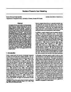
an associated payoff. Tasks can be decomposed into a set of subtasks. Subtasks are independent from one another but all subtasks must succeed for a mediator to receive the promised payoff. Different agents have different capabilities, hence subtasks may take different durations (depending on the agents assigned to them). The duration is also stochastic (though its mean may depend on the assigned agent). Subtasks also incur costs that need to be covered by the overall payoff for the total task to be profitable. The goal of the mediator is to maximize its net profit (maximizing payoff and minimizing cost). In general, mediators may interact with each other in the system, as shown in Figure 1. However, from a mediator’s perspective, it receives task announcements and contracts out subtasks to neighboring agents, independent of whether the other agents are mediators or not. Task

agent mediator

the payoff for the newer task and its expected duration and cost.

The decisions above are further complicated by the fact that subtasks’ costs and durations are stochastic with a distribution that is not known to the mediator a prior. We show how to model these decisions efficiently by generalizing the Semi-MDP model (SMDP)[8] and extending the Concurrent Action Model (CAM)[5]. We also present an algorithm that uses this model and reinforcement learning techniques to learn an optimal policy for a mediator. Section 2 presents an example to illustrate the mediator decision problem. Section 3 briefly describes the SMDP model and how it can be used to model serialized mediation. Section 4 shows how the SMDP model can be generalized to efficiently model randomly available actions. Section 5 describes how CAM can be extended to model concurrent mediation of subtasks. Section 6 shows experimental results illustrating how our model outperforms existing models when used to learn an optimal policy.

2. Task

Task

Task

Figure 1: A network of mediators for assigning agents to tasks. Although this work’s focus is on formalizing the decision process of a single mediator, this is done in a multi-mediator context. In particular, when a mediator m1 asks another mediator m2 to do a task T1 , m2 needs to decide as soon as possible whether to accept or reject T1 so that m1 can also decide its course of action. Consequently, a mediator cannot defer its decision about a task and queue it for consideration later. This constraint makes the mediator decision problem more challenging as the mediator needs to make a decision now that may affect its future profit. With this in mind, our work provides a formal decision theoretic model that enables a mediator to evaluate quantitatively the following three decisions.

EXAMPLE

Let us consider a simple mediator example illustrated in Figure 2. A mediator m can negotiate with four agents a0 , a1 , a2 , and a3 . Each agent ai can execute a single subtask Tai . The duration and the cost of a subtask Tai are stochastic and unknown to the mediator (but they depend on agent ai ). They are represented by random variables Dai and Cai respectively. At any given time, there is a set of available tasks T = {T0 , ..., Tn } available to m to choose from to mediate. Each task Tk can be decomposed into a set of subtasks Tk = {Tai , Taj , ...} and has a promised reward Rk (both are known to the mediator).

Figure 2: The experiment scenario • How a mediator should select among available tasks, where their subtasks are contracted out concurrently. The mediator should take into account that subtasks may have different durations depending on the agents assigned to the subtasks. Furthermore, no reward will be given until all subtasks are complete. • The mediator needs to decide between committing now to a task or waiting for a better task to arrive in the future. This decision is particularly important if the mediator cannot decommit a task once committed. The mediator needs to take into account the payoff of currently available tasks, their duration, and the likelihood of a better task arriving before any of the current tasks finish. • If decommitment is allowed, and the mediator receives a new task announcement, it needs to decide whether it is better to continue with an old task or decommit from the old task and start a new one. This decision needs to take into account the costs already accrued for performing the old task, the payoff for its completion, the expected time for the old task to finish,

The probability that a task of type Tk is available for mediation (at any point of time) is pTk . If a task type is not selected for mediation it may or may not be available at the next time step depending on pTk . For simplicity, assume the mediator can only mediate one task at a time. Consider an example scenario involving two tasks T0 = {Ta0 , Ta1 } and T4 = {Ta1 , Ta3 }. At time 0 task T0 is the only available task. m starts mediating T0 with agents a0 and a1 . At time 5 mediation about Ta1 finishes with cost ca1 . At time 7 another task T4 arrives while the mediation about subtask Ta0 has not finished yet. What should m do? If decommitment is allowed then m needs to consider whether to drop T0 and start T4 . Ignoring the effect of duration, m should drop T0 if the profit of T4 is higher, i.e., R0 − ca1 − E{Ca0 } < R4 − E{Ca1 } − E{Ca3 }, where E{X} is the expectation of random variable X. The above decision rule is not actually optimal as it ignores the effect of duration. For example, if the expected duration of Ta3 is 20 while the expected duration of Ta0 is 10, it would be better for m to stick with T0 even if the profit is lower as this will free m to accept another task earlier.

Now consider if m is not allowed to decommit a task once it started mediation. The mediator still has an interesting decision to make: whether to wait for a better task or not. For example in the previous scenario, if E{Da0 } = 30 while E{Da3 } = 5, then m would be better off not accepting T0 even if at the time m has nothing else to do and wait for T4 to arrive. Clearly making such a decision depends on the arrival rate of different tasks. For example, if T4 tasks arrives on average every 100 time units, m may be better not waiting for it, while if it arrives every 10 time units it might be worth the wait. Integrating all these factors into one coherent and simple model is a challenging task. The next section describes the Semi-MDP model which we use as a basis for modeling the mediator’s decision.

3. SEMI MARKOV DECISION PROCESS, SMDP The Semi-MDP [8], or SMDP, provides a basis for modeling an agent’s decision if the agent’s actions may take different durations. An SMDP is defined by the tuple hS, A, P, Ri. S is the set of states, A(s) is the set of actions available at a given state, P (s, a, N, s0 ) is the probability of reaching state s0 after N time-steps of executing action a at state s, and R(s, a) is the average reward if action a is executed at state s. The solution to an SMDP decision problem is an optimal policy π ∗ (s) that specifies for every state s what is the best action to execute. The optimal value of action a at state s, Q∗ (s, a) is the expected sum of rewards if the agent first execute action a then follows the optimal policy thereafter. Q∗ (s, a) is given by Bellman’s equation [8]: X Q∗ (s, a) = R(s, a) + P (N, s0 |s, a)γ N maxa0 Q∗ (s0 , a0 ) N,s0

where γ is a learning parameter called the discount factor. Another variant of this equation which is used in the Q-learning algorithm [7] is Q∗ (s, a) ← (1 − α)Q∗ (s, a) + α[R(s, a) + γ N maxa0 Q∗ (s0 , a0 )], where α is another learning parameter called the learning rate. Once the values of Q∗ are learned, the optimal policy can be easily computed: π ∗ (s) = argmaxa Q∗ (s, a). The mediator decision problem can be formulated using an SMDP as follows. The state s would be a combination of the states of its neighboring agents (or some abstraction of it) and the status of task(s) the mediator is pursuing. An action corresponds to the process of assigning a subtask to an agent. The task payoff is the reward received when the status of the pursued task is completed successfully. This is true iff all subtasks complete successfully. Every time-step a subtask may produce a reward r that is usually (but not necessarily) negative to represent the cost of doing the subtask. The SMDP model above can handle serialized contracting of subtasks. It can correctly model mediations with variant durations. However, this model does not explicitly handle concurrent actions and therefore can not handle concurrent mediation of subtasks. Mediating subtasks in parallel means some of them may finish earlier than others (since subtasks have variant durations). Shall the mediator wait for other subtasks to finish before making a new decision or shall it reconsider its decision whenever a subtask finishes? CAM [5], addresses these issues for the Semi-MDP model with concurrent actions. Section 5 briefly describes CAM and how to extend it to account for stochastically changing set of avail-

able actions. The following section proposes a generalization of the SMDP model that enables more efficient representation of the class of decision problems where the set of actions changes nondeterministically (i.e., the randomly available actions property).

4.

RANDOMLY AVAILABLE ACTIONS

In the SMDP model, the set of available actions At at time t is defined by a deterministic function A(st ) where st is the state at time t. In other words, the SMDP model requires the set of available actions at any time to be deterministically defined by the agent’s state. In the task allocation decision problem, the set of available actions At corresponds to the set of available tasks at time t. Because tasks arrive in a non-deterministic fashion, the only way to satisfy the SMDP model requirement of having a deterministic function A(s) is to include the set of available tasks as part of the state. While compatible with the traditional SMDP, this results in an exponential explosion in the number of states that hinders learning. However, it is intuitive that in some domains the value of an action is independent of other available actions (we prove this below). However, requiring the set of available actions to be a deterministic function of the current state is over constraining. We propose a generalization of the SMDP model, ℘-SMDP, which allows the set of available actions At at time t to be non-deterministically dependent on the current state of the agent. As we show below, this generalized model allows exponential savings in the state space. ℘-SMDP is defined by the tuple hS, ℘, P, Ri, where S, P, and R are as described in the previous section, while ℘(A|s) is the probability that the set of actions A is available at state s. The ℘(A|s) replaces the traditional A(s) function allowing more flexibility in the model. Mapping a traditional SMDP to ℘-SMDP is straightforward. S, P, and R are the same. ℘(A(s)|s) = 1 and ∀A 6= A(s) ℘(A|s) = 0. For clarity, we will use the symbol ℘ to refer to probabilities associated with actions. For example, ℘(At+N = A0 |st+N = s0 , st = s) is the probability that the set of available actions at time t + N is A given that the state at time t + N is s0 and the state at time t is s. We will also omit random variables when possible, i.e. ℘(At+N = A0 |st+N = s0 , st = s) = ℘(A0 |s0 , s). The real benefit of ℘-SMDP over the original SMDP is not its generality, but that under certain assumptions ℘-SMDP leads to a more compact representation of the Bellman equations as we show below. In particular, it is possible in the ℘-SMDP to factor the set of available actions out of the state. This leads to exponential savings in the state space and hence reduces the memory and time required to learn an optimal policy. Let s be the state with the set of available actions factored out while hA, si be the state with the set of available actions factored in. Let A and A0 be the set of available actions at time t and t + N respectively. Also s and s0 are the state at t and t + N respectively; and a and a0 are actions at t and t + N . T HEOREM 1. : If the following is true: • action independence: the set of available actions at time t can be dependent only on the current state, and is independent of all other variables given the current state. So for example, ℘(A0 |N, s0 , hA, si, ai ) = ℘(A0 |s0 ).

• outcome independence: the outcome of applying an action a in a given state s does not depend on the set of available actions at that time, i.e. P (N, s0 |A, s, a) = P (N, s0 |s, a) then the equation below is also true: Q(hA, si, ai ) = Q(s, ai ) = R(s) + X ℘(A0 |s0 )P (N, s0 |s, ai )γ N maxa0i ∈A0 Q(s0 , a0i ) N,A0 ,s0

P ROOF. Using Bellman’s equation, Q(hA, si, ai ) = R(s) + X P (N, hA0 , s0 i|hA, si, ai )γ N maxa0i ∈A0 Q(hA0 , s0 i, a0i ) N,A0 ,s0

but, using the Probability Product rule, P (N, hA0 , s0 i|hA, si, ai ) = ℘(A0 |N, s0 , hA, si, ai )P (N, s0 |hA, si, a℘(A0 |N, s0 , hA, si, ai ) P (N, s0 |hA, si, ai )i ) then, using the action independence assumption for the first part and the outcome independence for the second part, = ℘(A0 |s0 )P (N, s0 |s, ai ) and hence Q(hA, si, ai ) = R(s) + X ℘(A0 |s0 )P (N, s0 |s, ai )γ N maxa0i ∈A0 Q(hA0 , s0 i, a0i )

(1)

N,A0 ,s0

where parameter A in Q(hA, si, ai ) does not appear in the r.h.s., therefore Q(hA, si, ai ) = Q(s, ai ). Thus we can substitute Q(hA0 , s0 i, a0i ) = Q(s0 , a0i ) in (1). Note that the action-independence and outcome-independence assumptions are not as restrictive as it may first appear. The reason is that we did not impose any restriction on the state definition, allowing trade-off between compactness and accuracy. For example, in many domains the set of available actions may include the action the agent chose previously and is still executing (because the agent may choose either to continue the currently executing action or start a new action). In this case, it is sufficient to include the currently executing action as part of the state. The theorem above leads to compact representation of action values by factoring out the set of available actions. In other words, the values of all states that only differ in the set of available tasks are considered equal. This may lead, as the experiments show, to faster convergence using either dynamic programming methods (e.g. value iteration) or temporal difference methods (e.g. Qlearning). For completeness, Algorithm 1 shows how the value iteration algorithm [7] can be adopted (however, this work focuses on Q-learning). The corresponding update equation for Q-learning is Q(s, a) = (1 − α)Q(s, a) + α(R(s, a) + γ N ∗ maxa0 ∈A0 Q(s0 , a0 ) and the optimal policy π ∗ (A, s) = argmaxa∈A Q(s, a). Because the set of available actions is factored out of the state, the optimal action at any state is not unique. The optimal action depends also on the set

Algorithm 1: Value Iteration begin Initialize Q(s, a) arbitrarily, ∀a, s. repeat δ←0 for every state s and action a do q ← Q(s, a) Q(s, a) ← R(s, a)+ P 0 0 0 N 0 0 N,A0 ,s0 ℘(A |s )P (N, s |s, a)γ maxa0 ∈A0 Q(s , a ) δ ← max(δ, |Q(s, a) − q|) end until δ >  (small positive number) end

of available actions at that time. However, the optimal policy need not be stored explicitly. Instead, the optimal action at time t can be dynamically computed using Q(st , .) and At , where st and At is the state and set of available actions at time t respectively. Theorem 1 does not violate the conditions for convergence for Qlearning. In particular, Q-learning will converge with enough sampling of states and set of available actions, appropriately decaying learning rate, and bounded rewards [3]. Also since SMDP is a more generic model than MDP, the theorem holds for MDP.

4.1 The wait operator Having a dynamic set of available actions that stochastically changes over time raises an interesting decision question: whether an agent (mediator) should wait for a better action (task) to be available in the future or should the agent choose the best action (task) that is available now. One would expect that the probability distribution of the availability of actions (tasks), ℘, should affect such a decision. Our experiments in Section 6 verify this intuition. 5.

EXTENSION TO CONCURRENT ACTION MODEL

The Concurrent Action Model (CAM) [5] allows concurrent actions with different durations. The model builds on the Semi-MDP model. The action value equation of CAM is almost identical to that of the original SMDP model: X P (s, a ¯, N, s0 )γ N maxa¯0 Q(s0 , a Q(s, a ¯) = R(s, a ¯) + ¯0 ) N,s0

where the only difference is that a ¯ here is a set of concurrent actions (also called joint actions) instead of a single action. Thus using this model a mediator can contract out all subtasks in parallel, and this is considered a single joint action. The main contribution of [5] is the introduction of termination schemes which determine when the next decision cycle occurs. They defined three termination schemes: τany , τall , and τcontinue . The termination scheme τany means that an agent makes a new decision if any concurrent action finishes, possibly decommiting some of the unfinished actions (tasks). The termination scheme τcontinue is similar to τany but without decommitting. Finally, in τall the agent waits until all concurrent actions that started together to finish before making a new decision. It was proved that optimal policies learned using τany dominates both τall , and τcontinue [5]. In our case, the set of available actions may change at any time even if none of the currently executing actions have terminated. None of the termination schemes proposed in [5] account for that.

We propose the τchange termination scheme, in which a decision starts whenever an action terminates or the current state changes or the set of available actions change. In the task allocation problem τchange means a new decision is made when a mediation terminates or a new task arrives.

variables of the algorithm. Algorithm 3 generate actions for the set of available tasks. Algorithm 2: Learning 2.1 2.2

τchange is more suitable for multiagent settings where the state observed by an agent is not fully controlled by the actions of that agent. Other agents may change the system’s state unexpectedly. Next theorem compares the policy learned under τchange to a policy learned under other termination schemes proposed in [5]. Let Q∗τ be the optimal action values learned using termination scheme τ.

2.3 2.4

2.5

T HEOREM 2. The optimal policy obtained using τchange has a value that is higher than or equal to the value of the optimal policy using τany , or more formally: ∀s ∈ S, maxa¯ Q∗any (s, a ¯) ≤ maxa¯ Q∗change (s, a ¯)

2.6 2.7

P ROOF. For every policy π any obtained using τany termination scheme there exists a corresponding policy π change using τchange with the same value. π change can be obtained from π any simply by not changing the executed action unless an action terminates (i.e. repeating the previous action if the decision epoch was initiated due to a change in state or set of available actions).

2.8

2.9

In other words, the space of policies that can be learned using τchange dominates that of τany which in turn dominates τcontinue and τall . Figure 3 augments the figure in [5] with τchange policy space. Results shown in Section 6 show that in practice, the policy learned using τchange outperforms policies that use other termination schemes.

2.10 2.11 2.12 2.13

5.2

begin Initialization. s ← current state, a ¯ ∗last ← null, and slast ← null Let A ← generateActions() be the set of actions available at this time step with probability  (small positive number) let a ¯∗ ← random action ∈ A and with probability (1 − ) let a ¯∗ ← argmaxa¯∈A Q(s, a ¯).1 Let T ∗ be the task associated with a ¯∗ , and R∗ be the reward that will be gained if T ∗ is accomplished ¯∗last ) = If a ¯∗last 6= null then learn: Q(slast , a (1 − α)Q(slast , a ¯∗last ) + α[R + γ N Q(s, a ¯∗ )] Send negative response to rejected tasks: send reward Rf ail to all but the originator of T ∗ Start mediating subtasks of T ∗ with their assigned agents/neighbors as specified by the selected set of concurrent actions/assignments a ¯∗ Let R ← 0 and wait for the termination scheme condition to be satisfied after N time-steps (i.e., wait for all subtasks to finish in case of τall , any subtask to finish in case of τany , or any subtask to finish or any new task to arrive in case of τchange ) For every received response with reward rk from a neighbor k, R ← R + γ N rk If task T ∗ is accomplished (i.e. all subtasks succeed), then R ← R + R∗ slast ← s, a ¯∗last ← a ¯∗ Goto 2 end

Handling Multiple Tasks in Parallel

The concurrent action model can also be used to model a mediator who can mediate multiple tasks (and their corresponding subtasks) in parallel. Another level of joint actions is needed. Sub-actions in that level are tasks which in turn are joint actions of subtask mediations. For example, consider the scenario described in Section 2. Corresponding to tasks T0 and T4 the mediator has the joint actions ¯T4 = {aTa1 , aTa3 } respectively, where a ¯T0 = {aTa0 , aTa1 } and a aTai is the assignment hTai , ai i. To allow the mediator to negotiate about tasks T0 and T4 concurrently, another action needs to be ¯T4 }. a T0 , a added to the pool of available actions: a ¯ T0 ,T4 = {¯ Figure 3:

The relationship between policies learned using τall ,τcontinue ,τany , and τchange

The following section outlines an algorithm for the decision of the mediator. Part of the algorithm learns the optimal policy using the update equation described in Section 4. This algorithm is used in the experiments of Section 6.

5.1 Learning the Mediator’s Decision Process Algorithm 2 illustrates how mediators make decisions and learn the values of their actions. The main variables are: s, the current state, slast , the previous state, and a∗last , the action executed at slast . Steps 2.1-2.4 correspond to Q-learning (using a factored state). Steps 2.5-2.6 are the communication part, which can be modified if more complex protocol is desired. Steps 2.7-2.10 update the main

Figure 4 illustrates the hierarchy of action a ¯ T0 ,T4 . A different termination scheme can be assigned to each level of this hierarchy of joint actions. For example, the termination scheme for the subtasks level may be τall (wait for all subtasks to finish) while the termination scheme for the tasks level may be τany (if any task finishes, start mediating another one).

6.

RESULTS

We are interested in evaluating the performance of optimal policies under different termination schemes, with and without the wait operator, and under different distributions of loads. The experimental settings are as follows. The scenario described in Section 2 and pictured in Figure 2 is used. Data are averaged over 10 simulation runs, each consisting of 100,000 episodes (trials). The duration of each subtask is stochastic. With probability pi , agent i will finish

3.1 3.2

3.3

3.4 3.5

begin Every available task (at the current time) Ti has a set of decompositions Di . Each decomposition dj ∈ Di is a set of subtasks {T1 , ..., Tn } (In the simple example in Section 2, T0 has D0 = {d0 }, i.e., single decomposition, where d0 = {Ta0 , Ta1 }) A set of agent-subtask assignments, Adj , is generated for every decomposition. Each subtask assignment a ¯ ∈ Adj assigns every subtask in the decomposition dj to a neighboring agent, i.e., a = {hT1 , a1 i, ..., hTn , an i}, where ai here refers to an agent (in the example in the previous step, Ad0 = {¯ a0 } because every subtask can be assigned to only one agent, and a ¯0 = {hTa0 , a0 i, hTa1 , a1 i} A ← ∪ dj A dj ) end

Figure 4: The hierarchy of the joint action a¯ T0 ,T4

its subtask at this time step, and with probability 1 − pi it will not. Agents a0 and a2 have p = 0.2 while a1 and a3 have p = 0.8 (i.e. faster agents). Any subtask can take at most 10 time steps. Tasks, arriving to the mediator at time t, are selected randomly from all combinations of two subtasks (i.e. requiring two agents). Thus we have six different tasks shown in table 1. When any subtask is achieved the mediator gets a reward of -1 (cost). The wait operator has a reward of zero. When all subtasks of any task are achieved the mediator gets a reward of 16. Following our framework, contracting a task is modeled as a joint action consisting of two sub-actions. Each sub-action corresponds to assigning a subtask to an agent. Thus, the mediator has at its disposal 6 joint actions corresponding to table 1, as well as the wait operator which can be either enabled or disabled (described shortly).

Although not required by our model, we deliberately chose that all tasks and subtasks have the same reward so that the only criteria for evaluating a “good” task is its duration. Task T4 is on average the shortest as it consists of two subtasks that can be achieved by the two fast agents. T4 is available at any time with probability pT4 . Any other task is available with probability 0.2. Defining the state strikes a balance between optimality and speed of convergence. State consists of two parts. The first is the task currently being mediated, which is null if the mediator is idle. The second part is the actual progress of each action (i.e. the mediation process of each subtask). For simplicity our implementation uses the time elapsed while mediating each subtask. Although this state is not the most compact but it allows us to measure the trade-off between the optimality and the speed of convergence of different termination schemes. Note that in Q-learning, an agent learns only about states and actions the agent actually encounters. So for example, using the τall termination scheme, an agent will only learn about the first part of the state. The second part of the state is irrelevant because an agent makes its decision only when all subtasks terminate (either successfully or unsuccessfully). Using τany an agent will witness more states but not all of the states (e.g. at least one action must have terminated). An agent using τchange can potentially encounter all states and hence need to learn about all of them. Figure 5 shows the performance of different termination schemes when pT4 = 0.6 and the wait operator is disabled. As shown, the policy learned using τchange clearly outperforms those learned using τany or τall . It also converges faster. This was initially surprising as we expected the τchange policy to take more time to converge as it tunes the policy with finer granularity. But the reason τchange was able to quickly surpass the performance of τany and τall is that the short task T4 appears so frequently. This gives clear advantage to τchange which can interrupt an ongoing task (joint action) even before any subtask (single action) terminates.

all any

280

change

270 260

total reward

Algorithm 3: generateActions

250 240 230 220 210 200 190 0

20000

40000

60000

80000

100000

episodes

Figure 5: The performance of different termination schemes when Tasks T0 T1 T2 T3 T4 T5

a0 * * *

a1 *

a2

a3

* * * *

* *

* *

Table 1: Types of Tasks

pT4 = 0.6 and the wait operator is disabled

Figure 6 shows the performance of different termination schemes when pT4 = 0.6 and the wait operator is enabled. The wait operator significantly improves the performance of the τall policy and considerably improves the τany policy while slightly improves the performance of the τchange . With τall the mediator learns to wait for T4 type of tasks. The same is true for τany as it can decide to wait if T4 is not available. However, for τchange having the wait operator does not add much (as the mediator can interrupt a task taking too long anyway if there is a better task). In contrast, adding

wait as an additional action slows convergence as the agent need to learn about it as well.

p−SMDP SMDP 130 120

total reward

all any

290

change

280

total reward

270

110 100 90

260 80

250 70

240

0

20000

40000

230

60000

80000

100000

episodes

220 210 200 0

20000

40000

60000

80000

100000

episodes

Figure 8: The performance of the policy learned using τchange with available actions as part of the state (SMDP) and factored out of the state (℘-SMDP).

Figure 6: The performance of different termination schemes when pT4 = 0.6 and the wait operator is enabled

p−SMDP SMDP

124 122

total reward

120

Figure 7 compares the performance when pT4 = 0.1 and the wait operator enabled. Though the policy using τchange still outperforms other termination schemes, its convergence is considerably slower than the other two. The reason is that there are more decision epochs and states visited by τchange than the other two termination schemes (which is the same reason why τany converges slower than τall ), while the benefit of τchange in interrupting an ongoing task is reduced due to lower pT4 .

all any

135

change

130

118 116 114 112 110 108 106 0

20000

40000

60000

80000

100000

episodes

Figure 9: The performance of the policy learned using τall with available actions as part of the state (SMDP) and factored out of the state (℘-SMDP).

total reward

125 120 115 110 105 100 95 90 0

20000

40000

60000

80000

100000

episodes

Figure 7: The performance of different termination schemes when pT4 = 0.1 and the wait operator is enabled Figures 8 and 9 verify the theoretical results in Section 4. The convergence of the learned policies with the set of available actions factored out of the state (i.e. relying on ℘-SMDP model) is considerably faster than the learned policies with the set of available actions being part of the state. The reason is the size of the state space. When the set of available actions is part of the state, the mediator needs to learn about 32 times the number of states when the set of available actions is factored out. This slows convergence considerably, especially in the case of τchange (Figure 8) because the size of the state space, even when the of set available actions are factored out, is high.

the agent including: choosing a task to pursue among a set of available tasks, the detail with which to schedule a task, when to abort a task, when to start and stop a negotiation (mediation) with another agent. Though their decision problem is similar to ours, the approach taken is considerably different. They used the traditional MDP model, which is not scalable in the number of available tasks. Therefore, they had to limit the number of available actions at any time. Our ℘-SMDP model scales well with the number of available tasks. Also their model only handled serialized actions, while our model deals with concurrent actions. In [2], a mediator serially allocate tasks to agents. They used an MDP model where actions are agent-task assignments. This again differs from our concurrent allocation model, with different action durations. They also assumed that the set of tasks to be allocated are fixed and arrive in fixed order, while we assume tasks arrive stochastically. They also assumed agents with homogeneous capabilities, while our model supports heterogeneous agents.

7. RELATED WORK

The work in [1] modeled the resource allocation problem as a constrained MDP, or CMDP. A CMDP is an MDP augmented with a set of (resource) constraints. They did not support infinite horizon decision processes, unlike our model. The set of actions were assumed fixed and the policy was serial. They also used an offline algorithm which solved the problem assuming the transition probabilities are known.

The authors in [4] used an MDP model for the decision of a metacontroller. This meta-controller chose among high-level actions of

8.

CONCLUSION AND FUTURE WORK

We present in this work a single coherent Semi-MDP model of the challenging mediator decision problem. We propose the ℘-SMDP model, which is a generalization of the SMDP model, and we prove that ℘-SMDP model can lead to exponential savings in the memory and time required to learn an optimal policy. We also extended the concurrent action model with a new termination scheme that results in an optimal policy outperforming all previous termination schemes. This work lays the basic formal foundation for more interesting questions to be answered in the future. This work’s focus is on modeling the decision process of a single mediator. Evaluating the performance of our model and our algorithm in systems with a network of mediators is interesting and an ongoing work. The issues we intend to address include: how the network connections between mediators and agents affect performance, how the load of tasks arriving at one mediator affect the performance at another mediator, and how load balancing can be incorporated in our model. While our model can represent concurrent mediations as joint actions, the model is exponential in the size of the joint actions. This is clearly not scalable. We are currently investigating under what assumptions our model can be factored over tasks and how it affects optimality.

9.

REFERENCES

[1] D. Dolgov and E. Durfee. Optimal resource allocation and policy formulation in loosely-coupled markov decision processes. In In Proceedings of the Fourteenth International Conference on Automated Planning and Scheduling., 2004. [2] H. Hannah and A.-I. Mouaddib. Task selection problem under uncertainty as decision-making. In Proceedings of the first international joint conference on Autonomous agents and multiagent systems, 2002. [3] M. L. Littman and G. Szepesv´ari. A generalized reinforcement-learning model: Convergence and applications. In L. Saitta, editor, Proceedings of the 13th International Conference on Machine Learning (ICML-96), pages 310–318, Bari, Italy, 1996. Morgan Kaufmann. [4] A. Raja and V. Lesser. Meta-level Reasoning in Deliberative Agents. Proceedings of the International Conference on Intelligent Agent Technology (IAT 2004), September 2004. [5] K. Rohanimanesh and S. Mahadevan. Learning to take concurrent actions. Sixteenth International Conference on Neural Information Processing Systems (NIPS), 2003. [6] R. G. Smith. The contract net protocol: High level communication and control in a distributed problem solver. IEEE Transactions on Computers, 29(12):1104–1113, 1980. [7] R. Sutton and A. Barto. Reinforcment Learning: An Introduction. MIT Press, 1999. [8] R. S. Sutton, D. Precup, and S. P. Singh. Between MDPs and semi-MDPs: A framework for temporal abstraction in reinforcement learning. Artificial Intelligence, 112(1-2):181–211, 1999.