1 Department of Mathematics, University of California, Los Angeles, 520 Portola
Plaza, Los. Angeles, California ... INTRODUCTION. In many problems of image
analysis, we have an observed image f, representing a ... Malik [20], Alvarez et al.
Journal of Scientific Computing, Vol. 19, Nos. 1–3, December 2003 (© 2003)
Modeling Textures with Total Variation Minimization and Oscillating Patterns in Image Processing Luminita A. Vese 1 and Stanley J. Osher 1 Received May 2, 2002; accepted (in revised form) July 1, 2002 This paper is devoted to the modeling of real textured images by functional minimization and partial differential equations. Following the ideas of Yves Meyer in a total variation minimization framework of L. Rudin, S. Osher, and E. Fatemi, we decompose a given (possible textured) image f into a sum of two functions u+v, where u ¥ BV is a function of bounded variation (a cartoon or sketchy approximation of f), while v is a function representing the texture or noise. To model v we use the space of oscillating functions introduced by Yves Meyer, which is in some sense the dual of the BV space. The new algorithm is very simple, making use of differential equations and is easily solved in practice. Finally, we implement the method by finite differences, and we present various numerical results on real textured images, showing the obtained decomposition u+v, but we also show how the method can be used for texture discrimination and texture segmentation. KEY WORDS: Functional minimization; partial differential equations; oscillating functions; functions of bounded variation; finite differences; texture modeling; image analysis.
1. INTRODUCTION In many problems of image analysis, we have an observed image f, representing a real scene. The image f may contain noise (some random pattern of zero mean for instance) and/or texture (some repeated pattern of small scale details). The image processing task is to extract the most meaningful information from f. This is usually formulated as an inverse problem: given f, find another image u, ‘‘close’’ to f, such that u is a cartoon or simplification of f. In general, u is an image formed by homogeneous regions and with sharp boundaries. Most models assume the following relation between f and u: f=u+v, where v is noise or small scale repeated detail (texture), and extract only the u component from f. Usually, the component v is not kept, assuming that this models the noise. In this category, we mention Rudin, Osher, and Fatemi [22], Mumford and Shah [18], Perona and 1
Department of Mathematics, University of California, Los Angeles, 520 Portola Plaza, Los Angeles, California 90095-1555. E-mail: {lvese,sjo}@math.ucla.edu
553 0885-7474/03/1200-0553/0 © 2003 Plenum Publishing Corporation
554
Vese and Osher
Malik [20], Alvarez et al. [2], Chambolle and Lions [10], Aubert and Vese [5], among many others. These models have the ability of computing optimal piecewisesmooth approximations u of f, while noise or small repeated patterns are removed from the image. In some cases, the v component is important, especially if it represents texture. Texture can be defined as a repeated pattern of small scale details. The noise is also a pattern of small scale details, but of random, uncorrelated values. Both types of patterns (additive noise or texture) can be modeled by oscillatory functions taking both positive and negative values, and of zero mean [17]. Following the ideas of Yves Meyer [17], we show in this paper how we can extract from f both components u and v, in a simple total variation minimization framework of Rudin, Osher, and Fatemi [22]. The obtained decomposition can then be useful for segmentation of textured images and texture discrimination, among other possible applications. The textured component v is completely represented using only two functions (g1 , g2 ). This is much simpler and much more efficient than in other techniques for textures, which use a large number of channels to represent a textured image. To summarize, we propose in this paper a simple model, which combines the edge preserving model of ROF, with the texture preserving model of Y. Meyer. The technique used is by energy minimization and partial differential equations. We illustrate the benefits of the new decomposition on various numerical results and applications to texture discrimination and texture segmentation. We review next the main two ingredients of the proposed model: the total variation minimization of Rudin, Osher, and Fatemi (ROF) [22] for image denoising and restoration (see also Rudin and Osher [21]), and the space of oscillating functions introduced by Yves Meyer [17] to model texture or noise. Let f: R 2 Q R be a given image (we assume that the image initially defined on a rectangle in R 2, has been extended by reflection to the entire space). We assume that f ¥ L 2(R 2). In real applications, the observed image f is just a noisy version of a true image u, or (as we will see in this paper), it is a textured image, and u would be a simple sketchy approximation or a cartoon image of f. In the presence of additive noise, the relation between u and f can be expressed by the linear model, introducing another function v, and such that f(x, y)=u(x, y)+v(x, y). In the Rudin, Osher, and Fatemi restoration model [22], v represents noise or small scale repeated details, while u is an image formed by homogeneous regions, and with sharp edges. Given f, both u and v are unknown (if v is noise, we may know some statistics of v, such that it is of zero mean and given variance). In [22], the problem of reconstructing u from f is posed as a minimization problem in the space of functions of bounded variation BV(R 2), this space allowing for edges or discontinuities along curves. Their model, very efficient for denoising images while keeping sharp edges, is inf F(u)=F |Nu|+l F |f − u| 2 dx dy,
u ¥ L2
(1)
Modeling Textures with Total Variation Minimization
555
where l > 0 is a tuning parameter. The second term in the energy is a fidelity term, while the first term is a regularizing term, to remove noise or small details, while keeping important features and sharp edges. Existence and uniqueness results for the above minimization problem can be found in [1], [10], [25], [3] (see also [4]). This problem has minimizers in the space BV(R 2) of functions of bounded variation, which is defined by [11]: u ¥ BV(R 2) iff u ¥ L 1(R 2) and sup gF
3 F u div gF dx dy: gF ¥ C (R ; R ), |gF| [ 1 4 < .. 1 c
2
2
(2)
If we denote by v=f − u or f=u+v, then the above minimization problem can be written as: inf u ¥ BV
3 F(u)=F |Nu|+l ||v||
2 L2
4
, f=u+v .
(3)
Formally minimizing F(u) yields the associated Euler–Lagrange equation
1 2
1 Nu u=f+ div 2l |Nu|
(for a correct form of the equation 0 ¥ “F(u) satisfied by a minimizer u ¥ BV, we refer the reader to [25]). Nu In practice, to avoid division by zero, the curvature term div(|Nu| ) is approxiNu ), and the BV solution is obtained as the limit of smoother mated by div(` 2 2 E +|Nu|
minimizers, as E Q 0, as in [1], [25]. This convention will be always made in this paper. Then, the function representing noise or texture in the ROF model is Nu v=f − u=− 2l1 div(|Nu| ), but this is not computed explicitly in the ROF model. Only the component u is kept in the ROF model. Note that the above function v in the ROF model can be formally written ux uy , g2 =− 2l1 |Nu| . We have that as: v=div gF , where gF =(g1 , g2 ) and g1 =− 2l1 |Nu| g 21 (x, y)+g 22 (x, y)=2l1 for all (x, y), so that ||`g 21 +g 22 ||L . =2l1 (later we will use the notation |gF |=`g 21 +g 22 ). In [17], Yves Meyer proves that the ROF model will remove the texture, if l is small enough. In order to extract both the u component in BV and the v component as an oscillating function (texture or noise) from f, Yves Meyer [17] proposes the use of a space of functions, which is in some sense the dual of the BV space (see also condition (2)). On the topic of oscillations in non-linear analysis, we would also like to refer the reader to [19]. Y. Meyer introduces the following definition [17]: Definition 1. Let G denote the Banach space consisting of all generalized functions v(x, y) which can be written as v(x, y)=“x g1 (x, y)+“y g2 (x, y), g1 , g2 ¥ L .(R 2),
(4)
556
Vese and Osher
induced by the norm ||v||g defined as the lower bound of all L . norms of the functions |gF | where gF =(g1 , g2 ), |gF (x, y)|=`g1 (x, y) 2+g2 (x, y) 2 and where the infimum is computed over all decompositions (4) of v. Y. Meyer also gives the following three results [17]: Lemma 1. If v ¥ L 2(R 2), then |> f(x, y) v(x, y) dx dy| [ ||f||BV ||v||g . Lemma 2. If the norm of f in G does not exceed 2l1 , then the optimal Rudin, Osher, and Fatemi decomposition of f is given by u=0, v=f. Theorem 1. Let f, u, and v be three functions in L 2(R 2). If ||f||g > 2l1 , then the Rudin, Osher, and Fatemi decomposition f=u+v is characterized by the following two conditions: 1 ||v||g = 2l
and
1 F u(x, y) v(x, y) dx dy= ||u||BV . 2l
In the above results, we have used the notation ||u||BV :=> |Nu| for the total variation of u. Y. Meyer shows that, if the v component represents texture or noise, then v ¥ G, and proposes the following new image restoration model: inf
3 E(u)=F |Nu|+l ||v|| , f=u+v 4 . g
(5)
u
As was justified by Y. Meyer, we shall see that the space G allows for oscillating functions v, and the oscillations are well measured by the norm ||v||g . In the next section, we show how we can solve a variant of this model in practice, making use only of simple partial differential equations. Other work for restoration of textured images by total variation minimization in a wavelet framework is by Malgouyres [15, 16], Candés and Guo [29]. Also, texture modeling by statistical methods was proposed by Zhu, Wu, and Mumford, in [27, 28], and by Casadei, Mitter, and Perona in [7]. In the context of texture segmentation, we cite only a few related work, such as Koepfler, Lopez, and Morel [12], Sapiro [24], Lee, Mumford, and Yuille [14], Lee [13], Ballester and Gonzalez [6], among many other. A recent work for segmentation of textured images using segmentation based active contour models in a Gabor transform framework, is proposed by Sandberg, Chan, and Vese [23]. Finally, we would like to mention other work using u+v models, but in different contexts. One was proposed by Chambolle and Lions [10], where a given image f was decomposed into a sum u+v, such that u ¥ BV(W) and v was the smoother part of f, satisfying Nv ¥ BV(W)2 . Another related work involving image decomposition was proposed by Wells et al. [26], in the context of adaptive segmentation and classification using statistical methods: the new data Y=ln(X) (the logarithmic transformation of the initial data X), is decomposed into a sum of two other components, one being piecewise-constant (given by the mean intensities for each class) and the other one being an additive bias field, to represent intensity inhomogeneities.
Modeling Textures with Total Variation Minimization
557
2. DESCRIPTION OF THE MODEL We are motivated by the following approximation to the L . norm of |gF |=`g 21 +g 22 , for g1 , g2 ¥ L .(R 2): ||`g 21 +g 22 ||L . = lim ||`g 21 +g 22 ||L p . pQ.
Then, we propose the following minimization problem, inspired by (5): inf
3 G (u, g , g )=F |Nu|+l F |f − u − “ g − “ g | dx dy +m 5 F (`g +g ) dx dy 6 4 , 2
p
u, g1 , g2
1
2
2 1
x
1
y
2
1 p
2 p 2
(6)
where l, m > 0 are tuning parameters, and p Q .. The first term insures that u ¥ BV(R 2), the second term insures that f % u+div gF , while the third term is a penalty on the norm in G of v=div gF . Clearly, if l Q . and p Q ., this model is formally an approximation of the model (5) originally proposed by Y. Meyer. Formally minimizing the above energy with respect to u, g1 , g2 , yields the following Euler–Lagrange equations:
1 2 g +“ g 6 , g +“ g 6 .
1 Nu , u=f − “x g1 − “y g2 + div 2l |Nu|
5“x“ (u − f )+“ “ g =2l 5 (u − f )+“ “y
(7)
m(||`g 21 +g 22 ||p ) 1 − p (`g 21 +g 22 ) p − 2 g1 =2l
2 xx 1
2 xy 2
(8)
m(||`g 21 +g 22 ||p ) 1 − p (`g 21 +g 22 ) p − 2
2 xy 1
2 yy 2
(9)
2
In our numerical calculations, we have tested the model for different values of p, with 1 [ p [ 10. The obtained results are very similar. The case p=1 yields faster calculations per iteration, so we give here the form of the Euler–Lagrange equations in this case (p=1):
1 2 g +“ g 6 , g +“ g 6 .
1 Nu , u=f − “x g1 − “y g2 + div 2l |Nu| “ 5 (u − f )+“ “x `g +g g “ m =2l 5 (u − f )+“ “y `g +g m
g1 2 1
2 2
2
2 1
2 2
=2l
(10)
2 xx 1
2 xy 2
(11)
2 xy 1
2 yy 2
(12)
If the domain is finite, with exterior normal to the boundary denoted by (nx , ny ), the associated boundary conditions are:
558
Vese and Osher
Nu (n , n )=0, |Nu| x y (f − u − “x g1 − “y g2 ) nx =0, (f − u − “x g1 − “y g2 ) ny =0. As we shall see in the section devoted to numerical results, the proposed minimization model (6) allows to extract from a given real textured image f the components u and v, such that u is a sketchy (cartoon) approximation of f, and v=div(g1 , g2 ) represents the texture or the noise. In addition, the minimizer obtained for gF =(g1 , g2 ) allows us to discriminate two textures, by looking at the functions |gF |=`g 21 +g 22 , |g1 | or |g2 |. 2.1. Analytical Remarks We list here a few simple analytical remarks about the proposed models. We will use the following notation: for u ¥ BV, we denote its total variation by: ||u||BV :=> |Nu|. We assume that f ¥ L 2. • In the standard Rudin–Osher–Fatemi model [22], the residual is given by: f − u=−
1 K(u), 2l
Nu where K(u) denotes the curvature operator, defined by K(u)=div(|Nu| ).
• In the new model for p \ 1, the residual is given by the same expression: f − (u+v)=−
1 K(u). 2l
• In the new model with p=1, from equations (10)-(12), it is easy to show the following remarkable relation: m=|NK(u)|. • In the new model with p > 1, from Eqs. (7)–(9), we can easily show the following relations: m
`g +g 2 1 ||`g +g || 2 1
2 1
2 2
2 2 p
p−1
=|NK(u)|,
m ||`g 21 +g 22 ||p =F `g 21 +g 22 · |NK(u)|. If gF is of constant magnitude, then the above relation involves the BV norm of K(u), or the total variation of K(u). If gF is not of constant magnitude, then > |gF | · |NK(u)| can be viewed as a weighted BV norm of the curvature K(u).
Modeling Textures with Total Variation Minimization
559
• Lemma 3. If uˆ=0, gFˆ ¥ (L p) 2 is a minimizer of the problem (6), then ||f − div gFˆ ||g [ 2l1 . Proof. We will have for any u ¥ BV that: ||u||BV +l ||f − u − div gFˆ || 2L 2 +m || |gF | ||L p \ l ||f − div gFˆ || 2L 2 +m |||gFˆ |||L p , or ||u||BV +l ||u|| 2L 2 \ 2l F u(f − div gFˆ ) dx dy. Substituting in the above inequality u by Eu, and taking E Q 0, we obtain:
: F u(f − div gFˆ ) dx dy : [ 2l1 ||u||
BV
.
The conclusion follows from this last inequality and from the duality between BV and G 5 L 2. • Lemma 4. If uˆ ¥ BV, gFˆ =(0, 0) is a minimizer of the problem (6), then ||N(uˆ − f )||L q [ 2lm , with p1+1q=1. Proof. We will have for any gF ¥ (L p) 2 that: ||uˆ||BV +l ||f − uˆ − div gF || 2L 2 +m || |gF | ||L p \ ||uˆ||BV +l ||f − uˆ|| 2L 2 , or ||div gF || 2L 2 +m |||gF |||L p \ 2l F (f − uˆ) div gF dx dy=2l F N(uˆ − f ) · gF . Substituting in the above inequality gF by EgF , and taking E Q 0, we obtain:
: F N(uˆ − f ) · gF dx dy : [ 2lm || |gF| ||
Lp
.
The conclusion follows from this last inequality and from the duality between L p and L q. • Lemma 5. u=0 and gF =(0, 0) is a minimizer of the problem (6) iff ||f||g [ 2l1 and ||Nf||L q [ 2lm . Proof. The direct implication is a consequence of the two previous results. The converse implication can be also verified by the previous techniques. Remark. Lemma 3 could also be justified by applying Lemma 2 proved by Y. Meyer to fˆ=f − div gFˆ , for a fixed gFˆ . Remark. Finally, we can apply Theorem 1 to our minimization problem (6) for a fixed gF . Then, this reduces to the classical Rudin–Osher–Fatemi minimization
560
Vese and Osher
problem for a new data f − div gF , and we have the following property: for fixed gF , if ||f − div gF ||g > 2l1 and u is a minimizer, then ||f − u − div gF ||g =2l1 and 1 F u(x, y) f(x, y) dx dy − F u 2(x, y) dx dy − F u(x, y) div gF (x, y) dx dy= ||u||BV . 2l
Remark. We have verified some of these simple theoretical results by experimental calculations on simple images.
3. THE NUMERICAL DISCRETIZATION OF THE MODEL To discretize the Eqs. (7)–(9), we use a semi-implicit finite differences scheme and an iterative algorithm, based on a fixed point iteration. The equation in u is discretized following the schemes from [22] and [5]. Similar schemes are then used for the equations in g1 and g2 . The initial guess that we use for the iterative algofx fy rithm is as follows: u 0=f, g 01 =− 2l1 |Nf| , g 02 =− 2l1 |Nf| . The details of our numerical algorithm are as follows. We use the classical notations ui, j % u(ih, jh), fi, j % f(ih, jh), g1, i, j % g1 (ih, jh) and g2, i, j % g2 (ih, jh), where h > 0 is the step space and (ih, jh) denotes a discrete point, for 0 [ i, j [ M. To simplify the presentation, let us introduce the notation H(g1 , g2 )= (||`g 21 +g 22 ||p ) 1 − p (`g 21 +g 22 ) p − 2. The discrete forms of our equations are:
ui, j =fi, j −
g1, i+1, j − g1, i − 1, j g2, i, j+1 − g2, i, j − 1 − 2h 2h
r =1
1 + 2lh 2
−
=1
ui+1, j − ui, j h
2 +1 u 2
i, j+1
− ui, j − 1 2h
ui, j − ui − 1, j
ui, j − ui − 1, j h
r =1
1 + 2lh 2
−
ui+1, j − ui, j
=1 u
2 +1 u 2
i − 1, j+1
− ui − 1, j − 1 2h
2
2
ui, j+1 − ui, j ui+1, j − ui − 1, j 2h
i+1, j − 1
2 +1 u 2
− ui, j h
i, j+1
ui, j − ui, j − 1 − ui − 1, j − 1 2h
2 +1 u 2
i, j
− ui, j − 1 h
2
2
2
2
s 2
s
2
,
Modeling Textures with Total Variation Minimization
mH(g1, i, j , g2, i, j ) g1, i, j =2l
5u
i+1, j
561
− ui − 1, j fi+1, j − fi − 1, j g1, i+1, j − 2g1, i, j +g1, i − 1, j − + 2h 2h h2
6
1 + 2 (2g2, i, j +g2, i − 1, j − 1 +g2, i+1, j+1 − g2, i, j − 1 − g2, i − 1, j − g2, i+1, j − g2, i, j+1 ) , 2h mH(g1, i, j , g2, i, j ) g2, i, j =2l
5u
i, j+1
− ui, j − 1 fi, j+1 − fi, j − 1 g2, i, j+1 − 2g2, i, j +g2, i, j − 1 − + 2h 2h h2
6
1 + 2 (2g1, i, j +g1, i − 1, j − 1 +g1, i+1, j+1 − g1, i, j − 1 − g1, i − 1, j − g1, i+1, j − g1, i, j+1 ) . 2h
We introduce the following linearized equations:
u n+1 i, j =fi, j −
g n1, i+1, j − g n1, i − 1, j g n2, i, j+1 − g n2, i, j − 1 − 2h 2h
1 + 2lh 2
−
=1 u
1 + 2lh 2
−
mH(g n1, i, j , g n2, i, j ) g n+1 1, i, j
=1 u u =2l 5
r=1
u ni+1, j − u n+1 i, j u ni+1, j − u ni, j h
2 +1 u 2
n i, j+1
− u ni, j − 1 2h
n u n+1 i, j − u i − 1, j n i, j
−u h
r =1
n i − 1, j
2 +1 u 2
n i − 1, j+1
− u ni− 1, j − 1 2h
2
u ni, j+1 − u n+1 i, j u ni+1, j − u ni− 1, j 2h
2 +1 u 2
n i, j+1
− u ni, j h
n u n+1 i, j − u i, j − 1 n i+1, j − 1
n i+1, j
2
− u ni− 1, j − 1 2h
2 +1 u 2
n i, j
− u ni, j − 1 h
2
2
2
2
s 2
s
2
,
n − u ni− 1, j fi+1, j − fi − 1, j g n1, i+1, j − 2g n+1 1, i, j +g 1, i − 1, j − + 2h 2h h2
6
1 + 2 (2g n2, i, j +g n2, i − 1, j − 1 +g n2, i+1, j+1 − g n2, i, j − 1 − g n2, i − 1, j − g n2, i+1, j − g n2, i, j+1 ) , 2h mH(g n1, i, j , g n2, i, j ) g n+1 2, i, j =2l
5u
n i, j+1
n − u ni, j − 1 fi, j+1 − fi, j − 1 g n2, i, j+1 − 2g n+1 2, i, j +g 2, i, j − 1 − + 2h 2h h2
6
1 + 2 (2g n1, i, j +g n1, i − 1, j − 1 +g n1, i+1, j+1 − g n1, i, j − 1 − g n1, i − 1, j − g n1, i+1, j − g n1, i, j+1 ) . 2h
562
Vese and Osher
Introducing the notations:
c1 =
=1 u
c2 =
=1 u
c3 =
=1
c4 =
1
n i, j
2 +1 u
n i − 1, j
2 +1 u
n i+1, j
−u h
2
n i, j+1
− u ni, j − 1 2h
2
,
1
n i, j
−u h
2
n i − 1, j+1
− u ni− 1, j − 1 2h
1
u ni+1, j − u ni− 1, j 2h
=1 u
2
2 +1 u 2
1 n i+1, j − 1
−u 2h
n i − 1, j − 1
n i, j+1
− u ni, j h
2 +1 u 2
n i, j
2
2
2
2
2
2
,
,
− u ni, j − 1 h
,
n+1 n+1 and solving in each equation for u n+1 i, j , g 1, i, j and for g 2, i, j respectively, we obtain:
R
u n+1 i, j =
1 1 1+ (c +c2 +c3 +c4 ) 2lh 2 1
S5
fi, j −
g n1, i+1, j − g n1, i − 1, j g n2, i, j+1 − g n2, i, j − 1 − 2h 2h
6
1 (c u n +c2 u ni− 1, j +c3 u ni, j+1 +c4 u ni, j − 1 ) , + 2lh 2 1 i+1, j
R
g n+1 1, i, j =
2l 4l mH(g n1, i, j , g n2, i, j )+ 2 h
S5
u ni+1, j − u ni− 1, j fi+1, j − fi − 1, j g n1, i+1, j +g n1, i − 1, j − + 2h 2h h2
6
1 + 2 (2g n2, i, j +g n2, i − 1, j − 1 +g n2, i+1, j+1 − g n2, i, j − 1 − g n2, i − 1, j − g n2, i+1, j − g n2, i, j+1 ) , 2h
R
g n+1 2, i, j =
2l 4l mH(g n1, i, j , g n2, i, j )+ 2 h
S5
u ni, j+1 − u ni, j − 1 fi, j+1 − fi, j − 1 g n2, i, j+1 +g n2, i, j − 1 − + 2h 2h h2
6
1 + 2 (2g n1, i, j +g n1, i − 1, j − 1 +g n1, i+1, j+1 − g n1, i, j − 1 − g n1, i − 1, j − g n1, i+1, j − g n1, i, j+1 ) . 2h As it can be noticed from the above formula, we have used the following approximation of the mixed derivatives: “ 2xy g1 (i, j) %
1 (2g1, i, j +g1, i − 1, j − 1 +g1, i+1, j+1 − g1, i, j − 1 − g1, i − 1, j − g1, i+1, j − g1, i, j+1 ), 2h 2
Modeling Textures with Total Variation Minimization
563
and similarly for g2 . We have also tested another approximation to the mixed derivatives, which is: “ 2xy g1 (i, j) %
1 (g +g1, i − 1, j − 1 − g1, i+1, j − 1 − g1, i − 1, j+1 ), 4h 2 1, i+1, j+1
which also gave good results. In practice, we set h=1 and in our computer algorithm, we employ another fixed-point method: instead of u ni, j , g n1, i, j and g n2, i, j , we always use the most recent value computed for each function at that point. At the boundary, we extend ui, j by reflection outside the domain, and a simple boundary condition for gF would be Dirichlet boundary condition, which appears to work well in practice. We perform about 100 iterations for each experimental result. Other implicit or explicit schemes could have been constructed and used.
4. NUMERICAL RESULTS In this section, we show various numerical results using the proposed model. In all results, we take the space step h=1, and we perform 100 iterations in most cases. Since in practice we have not noticed differences between the cases p=1 and p > 1, we show the numerical results obtained with p=1. In Fig. 1 we consider a real textured image without noise for the initial data f. In Fig. 2 left we show the result u obtained with the ROF model, and in Fig. 2 right we show the residual f − u (plus a constant for illustration purposes). We see that texture (in form of geometry) is still present in the residual f − u. Next, in Fig. 3 we show the results obtained with the new model, for the same parameter l. Note from Fig. 3 that u+v represents very well the initial textured image f, and that in the residual f − u − v there is much less geometry and texture than by the ROF model. As expected, the image u in Fig. 3 is a sketchy approximation of f, while v is an oscillatory function (again, we have added a constant to the result v, for illustration purposes).
Fig. 1. An initial textured image.
564
Vese and Osher
Fig. 2. Result using the ROF model with l=0.1.
Fig. 3. Result using the new model with l=0.1, m=0.1.
Fig. 4. An initial fingerprint image.
Modeling Textures with Total Variation Minimization
Fig. 5. Result using the ROF model with l=0.1.
Fig. 6. Result using the new model with l=0.1, m=0.1.
Fig. 7. Original fingerprint image (left) and a noisy version f (right).
565
566
Vese and Osher
Fig. 8. Result using the ROF model with l=0.03.
Similar results and comparisons are presented in Figs. 4–6, for another textured image without noise, representing a fingerprint. Then, we show comparisons and numerical results for both models with a noisy fingerprint image, shown in Fig. 7. The result u obtained with the ROF model is presented in Fig. 8 left, and the residual in Fig. right. We see that the noise has been removed, but most of the texture is also removed from u. In Fig. 9 we show results obtained with the new model applied to the noisy fingerprint image, for various parameters m, but the same parameter l. Note that, as expected, the proposed model keeps together the texture and the noise for smaller m. It was also proved by Yves Meyer [17] that random additive noise of zero mean belongs to the same space G. So, the noise is considered as texture by the proposed model. Note that, for decreasing m, more texture appears in the v component by the new model, but also more noise is kept. In the next two examples (the fabric image and the wood image), we show that the new model can be used as a texture discriminator, by looking at the functions |g1 |, |g2 | or |gF |=`g 21 +g 22 . Even if the two textures are very similar, in these three components, their differences are clearly seen and can be discriminated. Also, note that in general, texture discrimination is very expensive, since the image f is substituted by a sequence of images, transforms of f at different scale, orientation and phase parameters (such as Gabor transforms), yielding a large set of initial data. Here, just one component suffices to discriminate textures, like |g1 |, |g2 |, or |gF |. In general, if we do not know which component(s) should be used, then at most three channels are needed for texture discrimination and texture segmentation, in a multi-channel segmentation fashion. Note that we do not need to perform a learning process of the texture and its statistics, as it is often done. Other methods for texture segmentation are using the so called ‘‘textons’’, as local averages of curvature of level lines and of the orientation of tangents to level lines (see for instance Koepfler, Lopez, and Morel [12] and Chan and Vese [9]).
Modeling Textures with Total Variation Minimization
Fig. 9. Results using the new model with l=0.03 and m=2; 1; 0.5; 0.1.
567
568
Vese and Osher
Fig. 10. Results on the fabric image with the new model, with l=0.01 and m=0.001.
Fig. 11. Results corresponding to the fabric image. Texture discrimination using the functions |g1 |, |g2 |, or |gF |. The detected contour is obtained by applying the active contour model without edges from [8, 9] to |g1 |.
Modeling Textures with Total Variation Minimization
569
Fig. 12. Results on the wood image with the new model, with l=0.1 and m=0.00001.
Fig. 13. Results corresponding to the wood image. Texture discrimination using the functions |g1 |, |g2 |, or |gF |. The detected contour is obtained by applying the active contour model without edges from [8, 9] to |g2 |.
570
Vese and Osher
Fig. 14. Left: f. Right: u+v with l=0.2, m=0.01, 100 iterations, p=1.
We show in Fig. 10 an initial image (fabric texture), and the results u+v, u and v obtained by the new model. In Fig. 11 we show the functions |g1 |, |g2 |, and |gF |. Here, we also show the contour between the two textures, extracted by applying the active contour model without gradient based segmentation from [8, 9] to the image |g1 |. Similar results are shown in Figs. 12 and 13, for another image (wood texture). Again, two of the functions |g1 |, |g2 |, and |gF | help to discriminate the textures. Finally, we show one more numerical result in Figs. 14 and 15. We show the initial image f (a noisy version of a real image), the result u+v and the u and v
Fig. 15. u (left) and v (right) components for the image in Fig. 14.
Modeling Textures with Total Variation Minimization
571
components. Note that u+v is practically identical with f. The noise is kept in the v component and therefore in the sum u+v, but it has been removed from the u component. Remark. Note that, since the residual |f − u − v| is very small but not exactly zero, the proposed model produces in fact a decomposition of the form: Nu f=u+v+r, where r=− 2l1 div(|Nu| ). In the limit, as l Q ., the model approximates a decomposition of the form f=u+v. 5. CONCLUDING REMARKS In this paper, we have shown how we can decompose a given image f into the sum u+v, where u ¥ BV is a function of bounded variation (a cartoon representation of f), and v is an oscillatory function, representing random noise or texture. We have also shown how the method can be used to texture segmentation and texture discrimination. The proposed model combines the idea of the total variation minimization in image restoration of Rudin, Osher, and Fatemi [22] with the ideas introduced by Meyer [17] for the appropriate space to model texture or noise. At this moment, the model cannot distinguish between noise and texture. We plan to discuss in the future how to denoise the v component, in the case of noisy textured images. Finally, we validate the claims of Yves Meyer on several experimental results, and we show in particular that textures can be defined and represented only using two functions gF =(g1 , g2 ). This is different from the wavelet decomposition techniques or from the use of the Gabor transform. ACKNOWLEDGMENTS The authors would like to thank Guillermo Sapiro for suggesting some related references, Eitan Tadmor for valuable conversations on this subject, and Richard Tsai, for discussions on the numerical discretization. L.A.V. was supported in part by NSF ITR-0113439, ONR N00014-02-1-0015, and NIH P20MH65166. S.J.O. was supported in part by NSF DMS-0074735, ONR N00014-97-1-0027 and NIH P20MH65166. REFERENCES 1. Acar, R., and Vogel, C. R. (1994). Analysis of bounded variation penalty methods of ill-posed problems. Inverse Problem 10, 1217–1229. 2. Alvarez, L., Guichard, F., Lions, P. L., and Morel, J.-M. (1993). Axioms and fundamental equations of image-processing. Archive for Rational Mechanics and Analysis 123, 199–257. 3. Andreu, F., Ballester, C., Caselles, V., and Mazon, J. M. (2000). Minimizing total variation flow. CRAS I-Mathématique 331(11), 867–872. 4. Andreu, F., Caselles, V., Diaz, J. I., and Mazon, J. M. (2002). Some qualitative properties for the total variation flow. J. Func. Anal. 188(2), 516–547. 5. Aubert, G., and Vese, L. (1997). A variational method in image recovery. SIAM J. Numer. Anal. 34(5), 1948–1979. 6. Ballester, C., and Gonzalez, M. (1998). Affine invariant texture segmentation and shape from texture by variational methods. J. Math. Imaging Vis. 9(2), 141–171.
572
Vese and Osher
7. Casadei, S., Mitter, S., and Perona, P. (1992). Boundary Detection in Piecewise Homogeneous Textured Images, Lecture Notes in Computer Science, Vol. 588, pp. 174–183. 8. Chan, T., and Vese, L. (1999). An active contour model without edges. In Scale-Space Theories in Computer Vision, Lecture Notes in Computer Science, Vol. 1682, pp. 141–151. 9. Chan, T. F., and Vese, L. A. (2001). Active contours without edges. IEEE Transactions on Image Processing 10(2), 266–277. 10. Chambolle, A., and Lions, P. L. (1997). Image recovery via total variation minimization and related problems. Numer. Math. 76, 167–188. 11. Evans, L. C., and Gariepy, R. F. (1992). Measure Theory and Fine Properties of Functions, CRC Press, London. 12. Koepfler, G., Lopez, C., and Morel, J.-M. (1994). A multiscale algorithm for image segmentation by variational method. SIAM J. Numer. Anal. 31(1), 282–299. 13. Lee, T. S. (1995). A Bayesian framework for understanding texture segmentation in the primary visual-cortex. Vision Research 35 (18), 2643–2657. 14. Lee, T. S., Mumford, D., and Yuille, A. (1992). Texture Segmentation by Minimizing VectorValued Energy Functionals—the Coupled-Membrane Model, Lecture Notes in Computer Science, Vol. 588, pp. 165–173. 15. Malgouyres, F. (2002). Mathematical analysis of a model which combines total variation and wavelet for image restoration, Journal of Information Processes 2(1), 1–10. 16. Malgouyres, F. (2001). Combining total variation and wavelet packet approaches for image deblurring. Proceedings, IEEE Workshop on Variational and Level Set Methods in Computer Vision, 57–64. 17. Meyer, Y. (2002). Oscillating Patterns in Image Processing and Nonlinear Evolution Equations, University Lecture Series, Vol. 22, Amer. Math. Soc. 18. Mumford, D., and Shah, J. (1989). Optimal approximations by piecewise smooth functions and associated variational problems. Comm. Pure Appl. Math. 42(5), 577–685. 19. Oru, F. (1998). Le rôle des oscillations dans quelques problèmes d’analyse non-linéaire, Thèse, CMLA, ENS-Cachan, June 9, 1998. 20. Perona, P., and Malik, J. (1990). Scale-space and edge-detection using anisotropic diffusion. IEEE on PAMI 12(7), 629–639. 21. Rudin, L., and Osher, S. (1994). Total Variation Based Image Restoration with Free Local Constraints, Proc. IEEE ICIP, Vol. I, Austin (Texas) USA, pp. 31–35. 22. Rudin, L., Osher, S., and Fatemi, E. (1992). Nonlinear total variation based noise removal algorithms. Physica D 60, 259–268. 23. Sandberg, B., Chan, T., and Vese, L. (2002). A Level-Set and Gabor-Based Active Contour Algorithm for Segmenting Textured Images, UCLA CAM Report 02-39. 24. Sapiro, G. (1997). Color Snakes. Computer Vision and Image Understanding 68(2), 247–253. 25. Vese, L. (2001). A study in the BV space of a denoising-deblurring variational problem. Applied Mathematics and Optimization 44(2), 131–161. 26. Wells, W. M., III, Grimson, W. E. L., Kikinis, R., and Jolesz, F. A. (1996). Adaptive Segmentation of MRI Data. IEEE Transactions on Medical Imaging, Vol. 15, No. 4. 27. Zhu, S. C., Wu, Y. N., and Mumford, D. (1998). Filters, random fields and maximum entropy (FRAME): Towards a unified theory for texture modeling. Intern. J. Comput. Vision 27(2), 107–126. 28. Zhu, S. C., Wu, Y. N., and Mumford, D. (1997). Minimax entropy principle and its application to texture modeling. Neural Computation 9 (8), 1627–1660. 29. Candés, E. J., and Guo, F. (2002). New multiscale transforms, minimum total variation synthesis: Applications to edge-preserving image reconstruction. Signal Processing 82, 1519–1543.