i.e., building a retrieval model based on user supplied labelled data. ... automatic image segmentation is a hard problem in computer vision and its solutions ... and we then want to use information from these specific regions to drive feedback.
Modeling User Feedback Using a Hierarchical Graphical Model for Interactive Image Retrieval Jian Guan and Guoping Qiu School of Computer Science, The University of Nottingham, UK {jwg, qiu}@cs.nott.ac.uk
Abstract. Relevance feedback is an important mechanism for narrowing the semantic gap in content-based image retrieval and the process involves the user labeling positive and negative images. Very often, it is some specific objects or regions in the positive feedback images that the user is really interested in rather than the entire image. This paper presents a hierarchical graphical model for automatically extracting objects and regions that the user is interested in from the positive images which in turn are used to derive features that better reflect the user’s feedback intentions for improving interactive image retrieval. The novel hierarchical graphical model embeds image formation prior, user intention prior and statistical prior in its edges and uses a max-flow/min-cut method to simultaneously segment all positive feedback images into user interested and user uninterested regions. An important innovation of the graphical model is the introduction of a layer of visual appearance prototype nodes to incorporate user intention and form bridges linking similar objects in different images. This architecture not only makes it possible to use all feedback images to obtain more robust user intention prior thus improving the object segmentation results and in turn enhancing the retrieval performance, but also greatly reduces the complexity of the graph and the computational cost. Experimental results are presented to demonstrate the effectiveness of the new method. Keywords: Image retrieval, image segmentation, graphical model, semisupervised learning, relevance feedback.
1 Introduction Reducing the semantic gap is one of the key challenges in image retrieval research. One popular approach is through user interaction where the user provides relevance feedbacks to the retrieval system which will then incorporate the user’s intention to refine the retrieval results to better match the user’s intention and expectation. Relevance Feedback, first used in document retrieval, was introduced into ContentBased Image Retrieval (CBIR) in early 1990s. A comprehensive review of relevance feedback in image retrieval can be found in [22]. One of the crucial problems in relevance feedback is modelling users’ feedback, i.e., building a retrieval model based on user supplied labelled data. There are two aspects to this problem. One is what (low-level) features to use to represent the image H.H.S. Ip et al. (Eds.): PCM 2007, LNCS 4810, pp. 18–29, 2007. © Springer-Verlag Berlin Heidelberg 2007
Modeling User Feedback Using a Hierarchical Graphical Model
19
content and the other is what algorithms to use for building the retrieval model. Early approaches mainly use global features; colour histogram and texture descriptors are the most commonly used. For the retrieval model, machine learning approaches such as Support Vector Machines (SVMs) are popular [8, 15]. In many situations, users are more likely looking for certain objects or parts of the images. Recent works by several authors e.g. [4, 17] have introduced region based approaches and achieve good results. To enable region based image retrieval, image segmentation algorithm is first employed to segment images into regions and then measure the similarity between the images using region-based features. There are two main obstacles to region based image retrieval (RBIR) approaches. Firstly, fullyautomatic image segmentation is a hard problem in computer vision and its solutions remains unstable and will remain so for the near future. Secondly, even if the segmentation results are satisfactory, we have no way of knowing which region is the one that the user is most interested in unless the user labels the segmented regions [4]. However, manually labeling the interested regions requires extra user effort. Such extra burden may be unacceptably heavy if the user has to label interested regions on more than one relevant image. To model the user’s intention in the relevance feedback process, specifically, we first want to find in the feedback images the regions that the users are interested in and we then want to use information from these specific regions to drive feedback features to refine image retrieval results. Suppose the user uses the image (a) in Figure 1 as a query image, which has been reasonably well-segmented, what is his/her intention? Is the user looking for images with a cow, or grassland, or lake, or all of them? Even another human user can not give the answer without other priors. Using relevance feedback, if the user supplies some more image samples, e.g. (d) and (e) in Figure 1, as positive feedback, it is very reasonable to assume that the user is actually interested in images with cows. Base on this intuition, some recent work e.g. [8, 9, 17] combine image segmentation and relevance feedback and obtain good results. However, these approaches rely on the performance of automatic image segmentation which is still a hard problem. Actually, we can make better use of relevance feedback. When the user selects some positive image samples, it is reasonable to assume that there is a common object or region across these images. This information can be used to refine the segmentation results and further reveal the user’s intention.
(a)
(b)
(c)
(d)
(e)
(f)
(g)
Fig. 1. What is the user’s intention? Assuming (a) is the querying image, when (d) and (e) are used as the positive feedback the segmentation result of (a) should be (b); when (f) and (g) are used as positive feedback the segmentation result of (a) should be (c).
This paper presents a novel framework for region based image retrieval using relevance feedback. The new framework is based around a novel hierarchical graphical model for simultaneously segmenting the positive feedback images into figure (user interested) and background (user uninterested) regions via a graph cut algorithm. The new model incorporates user’s intentions as priors, which not only can
20
J. Guan and G. Qiu
provide good segmentation performance but also will result in the segmented regions reflect user feedback intentions and can be readily exploited to perform image retrieval.
2 Extracting Relevant Objects and Features One of the drawbacks of the segmentation methods used in traditional region based image retrieval is that these methods usually segment an image into several regions. In some cases, one object could be divided into different regions. In other cases, even though the segmentation result is reasonably correct, e.g. image (a) in Figure 1, the retrieval methods need to figure out the region corresponding to the object which the user is interested in. Although the user can scribble on the interested objects, e.g. the cow or the grassland in Figure1 to indicate his/her intentions, we will address this scenario in future work whilst this paper will only study the use of statistical prior from the feedback images to model the user intention. In our approach, we do figure-ground segmentation, i.e. an image will be segmented into 2 regions only: the figure, which is the object the user intends to find, and the background. In the presence of relevance feedback as user supplied priors, the segmentation results are context sensitive as shown in Figure 1. In the case when a user uses image (a) as query image and supplies images (d) and (e) as positive samples, the segmentation result of (a) would be (b), where the figure is the cow; whilst using (f) and (g) as positive samples, the result would be (c), where the figure is the grassland. This result is to reflect the assumption that users are interested in the objects that occur most frequently in the positive feedback images. 2.1 CPAM Features The coloured pattern appearance model (CPAM) is developed to capture both colour and texture information of small patches in natural colour images, which has been successfully used in image coding, image indexing and retrieval [10]. The model built a codebook of common appearance prototypes based on tens of thousands of image patches using Vector Quantization. Each prototype encodes certain chromaticity and spatial intensity pattern information of a small image patch. Given an image, each pixel i can be characterized using a small neighbourhood window surrounding the pixel. This small window can then be approximated (encoded) by a CPAM appearance prototype p that is the most similar to the neighbourhood window. We can also build a CPAM histogram for the image which tabulates the frequencies of the appearance prototypes being used to approximate (encode) a neighbourhood region of the pixels in the image. Another interpretation of the CPAM histogram is that each bin of the histogram corresponds with an appearance prototype, and the count of a bin is the probability that pixels (or more precisely small windows of pixels) in the image having the appearance that can be best approximated by the CPAM appearance prototype of that bin. Such a CPAM histogram captures the appearance statistics of the image and can be used as image content descriptor for content-based image retrieval.
Modeling User Feedback Using a Hierarchical Graphical Model
21
2.2 A Hierarchical Graph Model A weighted graph G = {V, E} consists of a set of nodes V and a set of edges E that connect the nodes, where both the nodes and edges can be weighted. An st-cut on a graph divides the nodes into to 2 sets S and T, such that S T = V and S T = . The sum of weights of the edges that connect the 2 sets is called a cut, which measures the connection between the 2 sets.
∪
cut ( S , T ) = ∑∑ eij
∩ Φ
(1)
i∈S j∈T
The classical minimum cut problem (min-cut) in graph theory is to find the division with minimum cut amongst all possible ones [3]. figure
background terminals pk qk ……
prototypes
cik
wij
image
pixels
……
image
Fig. 2. A hierarchical graphical model jointly modeling pixels, appearance prototypes, figure and background.
If we view the pixels as nodes and the edges measure their similarity, figureground segmentation problem can be naturally formulated as a minimum cut problem, i.e. dividing the pixels into 2 disjoint sets with minimum association between them. This formulation has been used in, for example [14] for automatic single image segmentation using spectral graph cut, and [2] for semi-automatic single image/video segmentation with user scribbles using max-flow based method. We construct a hierarchical decision graph, as shown in Figure 2, where there are three types of nodes. At the lowest level are nodes corresponding to pixels in the images; at the intermediate level are nodes corresponding to the CPAM appearance prototypes; and at the highest level are two terminal nodes corresponding to figure and ground. The weighted edges measure the likelihood that two connected nodes fall in the same class, the figure or the background. In this way, we formulate the joint image segmentation problem as finding the minimum cut on the decision graph. Note that we only segment the query image and the positive samples which contain the desired objects to capture the user’s intention. Details are explained in the following subsections. 2.2.1 Intra-image Prior According to the image formation model, neighbouring pixels are highly correlated. When we divide an image into regions, two pixels close to each other are likely to fall
22
J. Guan and G. Qiu
into the same region. We measure the connection between two neighbouring pixels i and j in a single image using a widely adopted function [e.g. in 14] as follows.
wij = e
− d ( i , j )2 σ g2
e
− fi − f j
2
σ 2p
(2)
where d(i, j) is the spatial distance between the 2 pixels i and j; fi and fj are feature vectors computed around the pixels; σg and σp are the variances of the geometric coordinates and the photometric feature vectors. 2.2.2 Inter-image Prior From a high level vision perspective, similar objects in different images consist of similar pixels. Reversely, similar pixels in different images are likely to belong to the same object. Hence there should be connections between them in the decision graph. However, searching for similar pixels across the images is computationally intensive. Moreover, establishing edges amongst pixels in different images will make the graph dense and in turn exponentially increase the computational complexity. Instead, we introduce a new type of nodes as intermediate hops. Using the CPAM scheme described in section 2.1, each pixel can be associated with an appearance prototype, i.e., a small neighbourhood window of the pixel is encoded by an appearance prototype that is the most similar to the window. Without other prior knowledge, a pixel and its associated prototype should be classified similarly. In our graphical model, each prototype is a node; if pixel i is associated with prototype k, we establish an edge between them with a weight cik. The connection between them can be measure according to their distance. For simplicity, we set all cik = 1. Note that a pixel is connected to both its neighbouring pixels and a prototype, i.e. its status is affected by 2 types of nodes. To control the relative influences between the 2 different types of nodes, we introduce a factor λ1 and set all cik = λ1. In all the experiments, we find λ1 = 0.3 produce satisfactory results. 2.2.3 Statistical Prior The above two priors have not taken into account the information the user provides through relevance feedback. Decision made according to them would be ambiguous. We further introduce two special nodes, termed terminals, one represents the figure and the other represents the background. Furthermore, introducing these terminal nodes will enable us to make use of the max-flow algorithm [5] to cut the graph. Clearly, it would be difficult to establish links between terminals and pixels whilst it is possible to establish links between terminals and prototypes. We consider the scenario where user provides both positive and negative feedbacks and interpret them in such a way that there is a common (similar) object or region across the positive samples whilst the object does not exist in the negative samples. For each image m, we build a CPAM histogram hm as described in section 2.1. A summary histogram h+, named positive histogram, can be computed by adding the histograms of the query image and positive image samples. In the same way, we can compute a negative histogram h- from the negative image samples. To eliminate the influences of the image size and the sample size, all these histograms are normalized. Suppose the bin corresponding to the appearance prototype k counts bk+ in the positive
Modeling User Feedback Using a Hierarchical Graphical Model
23
histogram and counts bk- in the negative histogram, we could roughly estimate the probability that k belongs to the figure and background as:
p (k ∈ F ) ∝ bk+ and p (k ∉ F ) ∝ bk−
(3)
Thus we can further derive the connection between prototype k and terminal figure as pk=λ2p(k ∈ F) and that between k and background as qk=λ2p(k ∉ F), where λ2 is a factor that weight the influences between inter-image prior and statistical prior. In the implementation, we set λ2 as λ1 times the total pixel number in the query image and the positive image samples, in order to make the magnitude of edges connecting terminals and pixels approximately equal to each other. The underlying assumption here is that the desired objects in different images are similar to each other in the sense that they all consist of similar features whilst the background varies. Thus the size of the positive image sample set is large enough to make the features which indicate the desired object adequately significant. For example, in the case of finding human faces from an image database, if we simply use colour as feature, it could be expected that the colour of skin is the most significant in the statistic of positive samples. 2.3 Graph Cut Implementation Using the graphical model constructed above, we have successfully transformed the problem of finding the desired objects as the classical graph min-cut problem: dividing the pixels and prototypes into two disjoint sets with weakest connections between them, i.e. the two sets that are most unlikely belong to the same class, and each of the two sets connect to one of the terminals, respectively. According to [6], this is equivalent to the problem of finding the maximum flow between the two terminals figure and background. Note that the hierarchical graphical model proposed here is different from the one in [2] for interactive single image segmentation in two ways. Firstly, we have introduced a new layer consisting of feature prototype nodes whilst [2] only uses pixel nodes. Secondly, in [2], each node represents a pixel connects to both terminals whilst our pixel nodes are connected to prototypes only. Though the graph cut method proposed in [3] and used in [2] is also based on max-flow, it is optimized for the graphs where most nodes are connected to the terminals and more importantly, it does not has a polynomial bound for the computational complexity. Whilst in our case, only prototype nodes which take up less than 1% of the total number of the nodes are connected to the terminals. Instead, we use an improved “push-relabel” method H_PRF proposed in [5] in this implementation. According to [2] and [5], the method is known to be one of the fastest both theoretically and experimentally with a worst case complexity of O(n 2 m ) , where m = |E| and n = |V|. Clearly, compared to that in [2], the way we construct the hierarchical graph only slightly increases the number of nodes (by less than 1%) and significantly decreases the number of edges (by the total number of pixels). A recent work [11] which also uses max-flow method solves the problem of segmenting the common parts of two images, which requires that the histograms of the figures in the two images are almost identical. A novel cost function consisting of
24
J. Guan and G. Qiu
two terms was proposed, where the first one leads to spatial coherency within single image and the second one attempt to match the histograms of the two figures. The optimization process starts from finding the largest regions in two images of the same size whose histograms match perfectly via a greedy algorithm that adds one pixel at a time to the first and second foreground regions, and then iteratively optimize the cost function over one image whilst fix the other by turns. The assumption and the optimization process limits its application in image retrieval, where there are usually more than two positive samples and the object histograms might sometimes vary significantly (See Figure 3 for an example where there are both red and yellow buses). It is worth pointing out that our framework and solution is very different from these previous works. Since we emphasis more on capturing user intention than segmentation, we use simple features and weak priors only to illustrate the effectiveness of our hierarchical graph model framework. 2.4 An Iterative Algorithm The initial statistical prior described in section 2.2.3 is weak, where the positive histogram represents the global statistics of all positive image samples, whilst we actually intend to capture the features of the desired objects. When we obtain the figure-ground segmentation results, we can refine the estimation by computing the positive histogram h+ on the figures only and the negative histogram using both the negative samples and the background regions extracted from the positive samples. Then we update the weights of the edges connecting the terminals and the prototypes. Using the segmentation results obtained in the previous round to update the graph and cut the new graph, it usually takes no more than 3 iterations to converge and produces satisfactory results in our experiments. 2.5 Relevant Feature Selection Note that we only segment the query image and the positive samples which contain the desired objects to capture the user’s intention. In the retrieval phase, when we need to measure the similarity between two images, one or even both of them may not have been segmented. To measure the similarity of two un-segmented images, we can use global descriptors such as colour histogram, CPAM histogram, and other descriptors; and make use of the knowledge learned in the graphical model and weight the features appropriately. Given the joint segmentation results, we build a new positive histogram hw+ on all the figures, which captures the statistical characteristics of the desired object. We call hw+ weighting vector and use it to indicate the importance of difference feature prototypes. Note that some prototypes might weight 0 and will not affect the future decision. Let h be the original histogram, after relevant feature selection, the new relevant histogram hr is computed as hr = Wh, where W = diag(hw+).
3 Interactive Image Retrieval Using Semi-supervised Learning We use a graph-based semi-supervised method similar to that in [20] to perform interactive image retrieval. The query-by-sample image retrieval problem is tackled
Modeling User Feedback Using a Hierarchical Graphical Model
25
using a classification paradigm. Consider a given dataset consists of N images {x1, x2, …, xN}, we want to divide it into 2 classes where the first one C1 consists of the desired images and other images fall into the second one C0. For each image, we assume that there is an associated membership score, {(x1, α1), (x2, α2), …, (xN, αN)}, where 0 ≤ α i ≤ 1 is interpreted as follows: the larger α i is, the more likely xi belongs to C1; conversely, the smaller α i is, the more likely xi belongs to C0. Now consider the case where some of the samples are labeled, i.e., αi = yi, for i = 1, 2, …L, where yi ∈ {0, 1} is the class label of xi. The rest α L+1, α L+2, …, αN are unknown. Our task is to assign membership scores to those unlabeled data. Let αi defined above be the probability that a certain image xi belongs to C1. Let all images that can affect the state of xi form a set Si and call it the neighborhood of xi. In a Bayesian Inference framework, we can write:
α i = p ( xi ∈ C1 ) = ∑ p ( xi ∈ C1 | x j ∈ C1 ) p ( x j ∈ C1 )
(4)
j∈Si
(
)
Define δ ij = p xi ∈ C1 | x j ∈ C1 , then we have
α i = ∑ δ ijα j
∑δ
and
j∈Si
j∈Si
=1
ij
(5)
By making a mild assumption that the given data follow the Gibbs distribution, the conditional probabilities can be defined as follows
δ ij =
1 − β d ( xi , x j ) e Z
where
Z=
∑e
(
− βd xi , x j
j ∈S i
)
(6)
δ
where β is a positive constant, d(xi, xj) is a metric function, and ij = 0 for j∉Sj. In this paper, we use the weighted distance according to Equation (4) as the metric function and the scaling constant β was set as the inverse of the variance of all feature variables in Si. These definitions can be interpreted as a Bayesian decision graph where the nodes represent αi’s, and the weighted edge connecting two nodes xi and xj represent ij. Whilst others have hard classification in mind, e.g. using min-cut-based methods, we want to exploit the continuous membership scores directly and the benefits will become clear later. The task of classifying the data is therefore to compute the states of the nodes, αi’s, of the Bayesian decision graph. To make the 2nd equality of equation (5) holds, one need to collect all data that will have an influence on a given data point. Since the given dataset cannot be infinite and it is impossible and computationally unacceptable to find all images that will have an influence on a given xi, we cannot make the equality of (5) hold exactly. The best we can do is to make the quantities on both sides of equation (1) as close as possible. Therefore, the classification problem can be formulated as the following quadratic optimization problem:
δ
2 ⎧⎪ ⎛ ⎞ ⎫⎪ α = arg min ⎨∑ ⎜ α i − ∑ wi , jα j ⎟ ⎬ j∈Si ⎠ ⎭⎪ ⎩⎪ i ⎝
(7)
26
J. Guan and G. Qiu
To solve the optimization problem in (7), we use the labeled samples as constraints and solve for the unknown membership scores. For the labeled images, according to the definitions, we have αi = yi, for i = 1, 2, …L, where yi ∈ {0, 1}. Because the cost function is quadratic and the constraints are linear, the optimization problem has a unique global minimum. It is straightforward that the optimization problem yields a large, spares linear system of equations, which can be solved efficiently using a number of standard solvers and we use multi-grid method [7] with linear complexity in the implementation. Therefore, the formulation of the classification problem in an optimization framework has yielded simple and efficient computational solutions.
4 Experiments We performed experiments on a subset of the popular Corel colour photo collection. The dataset consists of 600 images divided into 6 categories: faces, buses, flowers, elephants, horses and aircrafts, each containing 100 images. Each image is represented by a CPAM histogram [10].
(a)
(b)
(c)
(d)
(e)
Fig. 3. Segmentation process of a “bus” image. 1st row: (a) the query image; (b) the segmentation result after the 1st round feedback; (c) an intermediate result of the 3rd round feedback; (d) final result of the 3rd round feedback, after applying the iterative algorithm described in Section 2.3; (e) result of Normalized cut [14]. 2nd row: some positive samples, the left 3 image are supplied in the 1st round and the right 3 are supplied in the 3rd round. 3rd row: some negative samples, the left 3 images are supplied in the 1st round and the right 3 are supplied in the 3rd round. 4th row: extracted relevance objects in the positive image samples.
In the experiments, we first choose one image from the dataset as query image and randomly pick 5 images from the same category as positive samples, and 5 images, one from each of the other five categories as negative samples. The query image and positive samples will be segmented and the weighting vector will be obtained using
Modeling User Feedback Using a Hierarchical Graphical Model
27
the hierarchical graphical model proposed in section 2 and then fed to the semisupervised learning interactive image retrieval technique described in Section 3 to produce the first round results. In the subsequent iterations, each time another 5 positive and 5 negative samples are supplied. In the following, we first present relevant object/region extraction/segmentation results, and then we will show the effectiveness of relevance feature selection, and finally report interactive image retrieval results. Figure 3 shows examples of segmenting out user interested objects from positive relevance feedback images. It is seen that when more and more samples are supplied by the user, the desired object becomes more and more significant whilst the background varies more and more. Hence the segmented figures become more and more homogeneous. In terms of human labour, our approach takes no more input than other Region-Based Image Retrieval methods that use relevance feedback [e.g. 8], where they use third-party automatic segmentation methods to segment the dataset off-line. In Figure 3, we also show the segmentation result of a state-of-the-art automatic segmentation technique [14] as comparison. These results illustrate that learning from relevance feedback can provide context-aware segmentation results that are much better than single image segmentation.
Fig. 4. Two images from the bus category. Left two: original images; Middle two: our results; Right two: results of [11].
We compare the object extraction ability of our method and the cosegmentation method of [11], results are shown in Figure 4. In general, our technique is able to extract object of interest and the accuracy increases as more iterations is used. Note that the results are produced under different conditions, where our results used 16 positive samples and 15 negative samples (see Figure 3) whilst those of [11] used only 2 images.
Fig. 5. Intra-class variances based on original features and weighted relevance features.
Fig. 6. Precision-Recall Curve of retrieving Bus category of images.
Fig. 7. Average PrecisionRecall Curves for all 6 categories after 3 iterations.
28
J. Guan and G. Qiu
As described in Section 2.5, once we have extracted relevant regions, we can weight the features of the image for relevant image retrieval. Figure 5 shows the intraclass variances using the global histograms via standard Euclidian distance and weighted histograms after 3 rounds of interactions. It can be seen that learning the feature weights from relevance feedback generally decreases the variance within each class. The improvement is especially significant for the categories that have large intra-class variances before relevant feature selection. To show the effectiveness of the method in interactive image retrieval, we plot precision-recall curves. Figure 6 shows an example result of retrieving the Bus category of images using the method detailed in Section 3. It is seen that the retrieval performance improves significantly in 3 rounds of interaction. SVMs have been extensively used in relevance feedback image retrieval [8, 15]. Figure 7 shows the precision recall performance of using SVM and the method of Section 3 (also see [20]) with both the original features and weighted features. It is seen that for both feedback methods, using our relevant feature selection improves the performances. These results demonstrate that our new framework for relevant region/object segmentation and relevant feature selection can effectively model the user feedback for improving interactive image retrieval.
5 Concluding Remarks In this paper, we have presented an innovative graphical model for modelling user feedback intentions in interactive image retrieval. The novel method embeds image formation prior, statistical prior and user intention prior in the edges of a hierarchical graphical model and uses graph cut to simultaneously segment all positive feedback images into user interested and user uninterested regions. These segmented user interested regions and objects are then used for the selection of relevant image features. An important feature of the new model is that it contains visual appearance prototype nodes which form bridges linking similar objects in different images which not only makes it possible to use all positive feedback images to obtain more robust user intention priors thus improving the object segmentation results but also greatly reduces the graph and computational complexity. We have presented experimental results which have shown that the new method is effective in modeling user intentions and can improve image retrieval performance.
References 1. Borenstein, E., Ullman, S.: Learning to segment. In: Pajdla, T., Matas, J.G. (eds.) ECCV 2004. LNCS, vol. 3024, Springer, Heidelberg (2004) 2. Boykov, Y., Jolly, M.P.: Interactive graph cuts for optimal boundary & region segmentation of objects in n-d images. In: Pro. ICCV 2001 (2001) 3. Boykov, Y., Kolmogorov, V.: An experimental comparison of min-cut/max-flow algorithms for energy minimization in vision. IEEE TPAMI 26, 1124–1137 (2004) 4. Carson, C., Belongie, S., Greenspan, H., Malik, J.: Blobworld: image segmentation using expectation-maximization and its application to image querying. IEEE TPAMI 24, 1026– 1038 (2002)
Modeling User Feedback Using a Hierarchical Graphical Model
29
5. Cherkassky, B.V., Goldberg, A.V.: On implementing push-relabel method for the maximum flow problem. Algorithmica 19(4), 390–410 (1997) 6. Ford, L.R., Fulkerson, D.R.: Flows in Networks. Princeton University Press, Princeton (1962) 7. Hackbusch, W.: Multi-grid Methods and Applications. Springer, Berlin (1985) 8. Jing, F., Li, M., Zhang, H.J., Zhang, B.: Region-based relevance feedback in image retrieval. IEEE Trans. on Circuits and Systems for Video Technology 14(5), 672–681 (2004) 9. Minka, T.P., Picard, R.W.: Interactive Learning Using A Society of Models. Pattern Recognition 30(4), 565–581 (1997) 10. Qiu, G.: Indexing chromatic and achromatic patterns for content-based colour image retrieval. Pattern Recognition 35, 1675–1686 (2002) 11. Rother, C., Kolmogorov, V., Minka, T., Blake, A.: Cosegmentation of Image Pairs by Histogram Matching - Incorporating a Global Constraint into MRFs. In: Proc. CVPR 2006 (2006) 12. Rui, Y., Huang, T.S.: Optimizing Learning in Image Retrieval. In: Proc. CVPR 2000 (2000) 13. Rui, Y., Huang, T.S., Ortega, M., Mehrotra, S.: Relevance feedback: A power tool in interactive content-based image retrieval. IEEE Trans. on Circuits and Systems for Video Technology 8(5), 644–655 (1998) 14. Shi, J., Malik, J.: Normalized cuts and image segmentation. In: Proc. CVPR 1997(1997) 15. Tong, S., Chang, E.Y.: Support vector machine active learning for image retrieval. In: Proc. ACM International Multimedia Conference (2001) 16. Vasconcelos, N., Lippman, A.: Learning from user feedback in image retrieval system. In: Proc. NIPS 1999 (1999) 17. Wang, J., Li, G., Wiederhold, G.: Simplicity: Semantics-sensitive integrated matching for picture libraries. IEEE TPAMI 23, 947–963 (2001) 18. Winn, J., Jojic, N.: LOCUS: Learning Object Classes with Unsupervised Segmentation. In: Proc. ICCV 2005 (2005) 19. Wood, M.E., Campbell, N.W., Thomas, B.T.: Iterative refinement by relevance feedback in content based digital image retrieval. In: Proc. ACM International Multimedia Conference (1998) 20. Yang, M., Guan, J., Qiu, G., Lam, K-M.: Semi-supervised Learning based on Bayesian Networks and Optimization for Interactive Image Retrieval. In: Proc. BMVC 2006 21. Yu, S-X., Shi, J.: Segmentation given partial grouping Constraints. IEEE TPAMI 26(2), 173–183 (2004) 22. Zhou, X.S., Huang, T.S.: Relevance feedback in image retrieval: A comprehensive review. Multimedia Syst. 8(6), 536–544 (2003)