models might be a way of interacting with the model on a computer. .... Figure 3: Different degrees of detail for the segmentation of a heart ventricle depicted by ...
Modelling, Visualization, and Interaction Techniques for Diagnosis and Treatment Planning in Cardiology Johannes Behr1, Soo-Mi Choi2, Stefan Großkopf3†, Helen Hong2, Sang-Ah Nam2, Yun Peng3, Axel Hildebrand1, Myoung-Hee Kim2, Georgios Sakas3 1
Computer Graphics Center (ZGDV), Dept. Visual Computing, Rundeturmstr 6, 64283 Darmstadt, Germany {Johannes.Behr,Axel.Hildebrand}@zgdv.de 2 Ewha Womans University, Dept. of Computer Science and Engineering, Seodaemun-gu, daehyundong 11-1, Seoul, Korea {choism,hlhong,sanam,mhkim}@mm.ewha.ac.kr 3 Fraunhofer Institute for Computer Graphics, Dept. Cognitive Computing & Medical Imaging, Rundeturmstr 6, 64283 Darmstadt, Germany {Stefan.Grosskopf,Georgios.Sakas}@fhg.igd.de
†
Corresponding Author
Abstract. Due to the development of new imaging devices, which produce a large number of tomographic slices, advanced techniques for the evaluation of large amounts of data are required. Therefore, computer-supported extraction of dynamic 3-D models of patient anatomy from temporal series is highly desirable. Since the diagnostician must be able to quickly make rational decisions based on the models, a high degree of accuracy is required within a minimum amount of time. We present modelling and visualization techniques that are realized within the Cardiac Station. Results for the application of these techniques to cardiac image data are given. In addition to providing information about the patient’s morphology, functional parameters can be derived from the data and visualized together with the model. In order to verify the model with the original image data and to plan for real intervention, interaction techniques are presented.
Keyords: Cardiology, Medical Imaging, Modelling, Visualization, ManMachine Interaction
2
Introduction Multi-slice spiral-tomographic imaging devices permit the acquisition of highresolution volumetric data sets of the dynamic heart. Due to high spatio-temporal resolution, these devices produce a large number of slices (approx. 500), which cannot be handled by evaluating each of the individual slices. Computer-supported creation of dynamic 3-D models of the patient’s anatomy from temporal series is thus highly desirable. The modelling aims at creating models that would otherwise need to be reconstructed mentally. In order to preserve the distinctiveness of medical images, emphasis has to be put on modelling accuracy, speed and detail of visualization, and interaction with the model. Ideally, the accuracy of models should be high enough to reproduce every detail of the original image data relevant for diagnosis. Whereas in other areas of Computer Graphics, esthetic aspects often are most important, in the area of medical imaging, results are measured in terms of usefulness for the diagnostician. Thus, visualization has to be efficient concerning rendering speed and accuracy. Since a single method is not suitable for showing every detail in adequate rendering time, two different methods are usually considered for medical imaging: • Surface rendering is a fast method, since it is supported by specialized hardware. The rendered images may lack important details, however. Thus, for medical applications, it is suited for previewing only. • Direct volume rendering is an established visualization method in medical imaging due to its high degree of detail. This method, however, usually lacks in performance and thus limits the degree of interactivity.
3
Figure 1: Example of a visualized cardiac EBCT data set: (a) maximum intensity projection (MIP), (b) surface rendered model of the left and right heart, (c) extraction of surfaces, and (d) MPR slice mapped on an oblique cutting plane. Besides providing an understanding of the morphology, medical imaging aims at extracting and visualizing additional information. This may consist of functional parameters, as in cardiology, the regional heart wall motion or information about the connectivity of vessels. Additional information is then derived from the image data by means of image processing methods and coded into the surface colour of the models. This technique is especially useful in the case of cardiology, since the alteration of cardiac wall motion during systolic contraction is one of the most sensitive indicators of cardiac disease, such as ischemia, and myocardial infarction. In this paper, we present results of an advanced method [1] for the modelling of the left ventricle endocardial motion during a cardiac cycle. As the colour-coded visualization provides a qualitative description of regional wall motion, the diagnostician may distinguish an abnormally contracting myocardium quickly and easily.
4
In addition to visualization, a model can be used to quantify diagnostic measures, e.g. ventricle volumes or the ejection fraction. These measures can be calculated with lower error from models than with conventional methods, since the latter are mostly based on simplifying assumptions, e.g. that a ventricle has the shape of an ellipsoid. Beneficial for diagnosis and treatment planning support, incorporating dynamic models might be a way of interacting with the model on a computer. Besides being able to rotate the model interactively in order to inspect it from all viewing directions, navigation through the original tomographic slices can be greatly simplified by interactive pointing and slicing operations. If the user clicks on a point on the model surface, the respective point should be shown in the original slices, e.g. mapped on a virtual cutting plane overlaid to the model (Figure 1). This leads to a better understanding of the relation between the model and the original image information and enables the comparison with the golden standard of tomographic imaging. Moreover, during a medical diagnosis and treatment planning procedure, a model can offer the following potentials: • Models can be used to fuse information from different imaging modalities. • Since a model can be represented by a reduced amount of data, it can be transferred more easily via network than the original image data for tele-consultation by a remote expert. • Using stereolithography, highly accurate plastic models of a patient’s anatomical structures can be created.
Processing Pipeline In this paper, we present a processing pipeline (Figure 2) that is realized within the Cardiac Station [2]. The Cardiac Station is being developed in a project [19], [21] at the Computer Graphics Center (ZGDV), the Fraunhofer Institute for Computer Graphics both at Darmstadt, Germany, in cooperation with the Ewha Womans University in Seoul, Korea. Some aims and concepts of the Cardiac Station are described in the last section of this paper in more detail. In an initial step, the tomographic slices are read from a PACS or a tomographic device in DICOM format. These slices can be piled up to volume blocks and rendered using direct volume rendering. Conventional volume rendering methods cannot solve the problem of occluding contours. It is, for example, impossible to visualize just a single ventricle, since the extraction of surfaces for rendering is based on the physical properties that are similar for both ventricles; thus, both ventricles occlude each other. In order to avoid occlusions during visualization, the slices are segmented to define contours of interest. The resulting stack of contours can in turn be integrated into a closed 3-D model by triangulation. Subsequently, the heart movement is tracked during the heart phase by finite element (FEM) tracking methods, resulting in a dynamic model. For a better interpretation of the data, motion parameters can be
5
estimated from the dynamic model and visualized with the model by encoding speed or acceleration as surface colour.
Figure 2: Processing Pipeline of the Cardiac Station
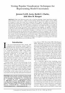
Segmentation Using Active Contour Models (ACM) Conventional segmentation techniques integrated into diagnosis and planning systems require the manual outlining of structures of interest on every single slice, or, additionally offer simple drawing support, like copying and pasting the contours from slice to slice, followed by manual adaptation of the contours. In order to reduce the user interaction required for the segmentation, the usage of active contour models (ACM) is realized within the Cardiac Station. These models support the segmentation through the integration of image features, like contours and homogeneous regions. ACMs are adaptive contour representations, also known as snakes or deformable models [5]. They are able to recover and represent physical contours of an image, due to their simulation of physical properties, like elasticity of material. They are widely applied for modelling object boundaries in static images, as well as for tracking in temporal image sequences, e.g. dynamic cardiac images [20], [6]. The main advantages of the ACM technique are the following. First, ACMs show robust behaviour for the segmentation of noisy images with sparse image features. They are able to interpolate fragmentary defined boundaries as a result of their elastic properties. Second, ACMs have the potential of integrating numerous local and global image features, knowledge-based constraints, and user-defined constraints into a closed mathematical model. Third, the segmentation result can be reproduced with predictable variances [2].
6
Figure 3: Different degrees of detail for the segmentation of a heart ventricle depicted by MRA by using different vertex distances for the adaptive B-spline. A wide variety of ACM-based approaches exists and several have been evaluated for cardiac images in previous works [2,3]. The simulation of Lagrangian dynamics (LD) proved to be the most robust approach. We will present this approach briefly. The ACM is represented by a parametric curve implemented as an adaptive B-spline [7] that adjusts the number of vertices to the curve length. Due to the adaptation of the number of vertices, the curve is able to fit image contours with a defined degree of detail even throughout changes of the total curve length (Figure 3). LD are simulated by assigning a mass, acceleration and velocity to each curve point. The curve is moved by application of two forces: acceleration force and damping force. The acceleration, velocity, and curve position are calculated iteratively using an explicit time integration scheme that is shown in equation (1) through (3).
∂ 2 v( s ) F (v( s )) = m( s ) ∂t 2
( 1 )
∂v( s ) ∂v( s ) ∂v( s ) ∂ 2 v( s ) − D(v( s )) = + ∆T 2 ∂t ∂t ∂t ∂t
( 2 )
v( s ) = v( s ) + ∆T
∂v( s ) ∂t
( 3 )
F: Acceleration force D: Damping force ∆T: Size of time interval The forces F and D are derived from image properties. We apply the result of the classification p(I(x,y)|α) in the direction of the curve normal as acceleration force F. If the pixel at curve point v(s) belongs with high probability to the region to be segmented, the curve is accelerated towards the border of this region. Additionally, the result of an edge enhancement operator (e.g. the length of the local image gradient
7
calculated by a Sobel filter) is added to a constant term of the damping force. As a result, oscillations of the curve around the region border are damped and the curve slows down when approaching a contour. This simple algorithm shows great robustness to overcome minor local minimums by accumulating kinetic energy. The main advantage of the LD approach is its great robustness to image noise. Choosing large distances between vertex points of the adaptive B-spline reduces the degree of freedom and the force along the ACM is accumulated. As a result, errorprone forces are suppressed, resulting in great robustness. Since the distribution of the contrast dye and the imaging parameters (especially for MRI) may change from slice to slice, one drawback is the need for adapting the region parameter α.
Figure 4: Results of segmenting using LD-based ACM on EB-CT slices (top: resulting contours; bottom: triangulated model). The results shown in Figure 4 have been produced by segmentation applying the LD approach. In a subsequent step, the stack of contours has been converted into a surface representation by an implicit surface triangulation algorithm. The result in Figure 4 is based on a static EBCT data set of 49 slices (5122 pixels). The left and right ventricle, parts of the left and right atriums, as well as some parts of the aorta and lung vessels, are included in the model. The time for the segmentation was
8
approx. 30 minutes. A large amount of time was required for the adaptation of the distribution model p(I(x,y)|α).
Ventricular Motion Simulation Medical imaging technologies can provide internal views of the cardiac ventricles and atria three-dimensionally, but the computer-aided visualization and analysis of four-dimensional images are still limited. In this sub-section, we present a new method for motion simulation of the left ventricle (LV) during a cardiac cycle. The colour-coded data of motion magnitudes are generated in a previous step or online, and are realistically visualized by a dynamic viewer on the computer screen. As colour-coded visualization provides a qualitative description for wall motion in clinically useful ways, diagnosticians may distinguish an abnormally contracting LV quickly and easily. Given the sets of 3D feature points on the surface of the LV, our goal is to create an accurate 4D model to simulate the motion dynamics of the LV. Our model decomposes the overall motion into global motion and local motion. At each time step, the model first finds the global motions, such as translation and rotation, and then deforms itself due to forces exerted by virtual springs, which are attached between the model and feature points extracted from images at the next time step. The most common numerical method to determine the dynamic equilibrium shape of the elastic body is the finite element method (FEM). The major advantage of the FEM is that the system can be expressed by interpolation functions that relate the displacement of a single point to the relative displacements of all the other nodes of an object. This provides an analytic characterization of shape and elastic properties over the whole surface and alleviates problems caused by irregular sampling of feature points [9]. The best choices of elements and interpolation functions depend on the object shape, degree of freedom, and trade-offs between accuracy and computational requirements. In our work, we chose a single 3-D blob element with a priori knowledge about the anatomic structure of the LV [8]. The geometric structure of the blob element begins with a superellipsoid that has the same size and orientation as the initial reference shape. It is triangulated according to the desired geometric resolution and then the vertices of triangles are employed as FEM nodes. We then introduce a new type of Galerkin interpolant based on 3-D Gaussians that allows us to efficiently solve motion tracking problems and compute robust canonical descriptions for data in 3-D space.
9
Figure 5: Tracking of the motion of the LV Detailed procedures to simulate the motion of the LV are shown in Figure 5. We start with a set of 3-D points at each time step during a cardiac cycle. The points are obtained from the surface of the LV, which has already been segmented. For a given set of 3-D points at initial time, we first create a superellipsoid model centered at the center of gravity and rotated into the principal axes. FEM nodes are superimposed on the initial model in order to unify geometric and physical information. The correspondence between 3-D points and model points is established by the bidirectionally closest method. Then, FEM mass, stiffness, and the mode shape vectors are computed. In general, the number of feature points from images will be greater than the number of modal displacements to be estimated; thus, we can solve them via weighted least squares. We can get a deformed model, therefore, by applying the calculated coefficients to the undeformed model points. The deformed model is translated into the new center of gravity of 3-D points, and is rotated into new principal axes at the next time step. After translation and rotation, the model is used for fitting at the next time step as an undeformed model. FEM node positions are also updated according to the calculated nodal displacements. After creating a 4-D motion model, we can extract cinematic attributes, such as displacement, speed or acceleration. Then, colour-coded data for wall motion magnitudes are superimposed to a 4-D geometry. As a result, by changing the coordinate data and colour, the LV can be animated over time. Figure 6 shows the
10
results of colour-coded LV. This colour-coded visualization can be used in medical education to show the effects of specific abnormalities on the heart.
Figure 6: Colour-coded visualization of the left ventricle
Visualization As a result of the various procedures, static and dynamic surface descriptions are generated. Therefore, the system must provide techniques to visualize the polygonal data. Since the hardware of a modern PC and workstation supports the rendering of 3D polygonal models, this description can be visualized very efficiently. A common drawback of polygon rendering, however, is the necessary reduction of information compared with the original slices. In addition, modelling procedures introduce slight approximation errors. In order to make a reliable diagnosis based on 3-D or higher dimensional visualization, the physician should be able to see all relevant information he or she can otherwise derive from studying the slices. Polygon rendering is thus not always appropriate to provide this diagnostically relevant information. It is more suitable to use polygonal rendering in order to receive a fast preview of the approximate shape, location, orientation, and movement of the given data to be evaluated. In many cases, direct volume rendering can produce more accurate images, but lacks performance. For these reasons, both methods, direct volume and surface rendering, are included in the Cardiac Station. Surface Rendering The triangulation module provides one polygonal surface description per segmented object. If the number of triangles of these models is very high, the data cannot be rendered efficiently in time and an appropriate reduction method must be applied.
11
Figure 7: Multi-resolution mesh visualization of a segmented heart (number of triangles: approx. 210,000; approx. 3,000; approx. 160). The most common polygonal reduction techniques generate a single static mesh based on an upper limit regarding the approximation error. Since the reduction process usually takes several minutes, the parameters cannot be adjusted interactively. To control the resolution of the mesh in real-time, we developed a method to generate a multi-resolution mesh from the triangulation results. In contrast to the previous reduction methods, the system does not store only one mesh as outcome, but a progressive mesh, which includes the information on how to simplify the mesh by collapsing edges for a given resolution [23][24][25]
Figure 8: Edge Collapse Transformation The progressive mesh is created in an initial processing step, which can be executed offline before any interaction process. Starting from the initial mesh, edges are consecutively collapsed to one of its end vertices. At each step, the edge causing the smallest visual change to the surface is selected. Small visual changes result by collapsing edges which are rather short and whose adjacent triangles are rather coplanar.
12
Hence, the edge having the minimum value of the cost function in equation (4) is collapsed.
1 − normal( f ) • normal(n) cost(a, b) = a − b × max min f ∈Ta n∈Ta ,Tb 2 with Ta : set of triangles containing the vertice a
( 4 )
Tb : set of triangles containing the vertice b In fact, collapsing an edge (Figure 8) replaces the occurrence of the vertex a in the triangle list by the vertex b, resulting in a mesh reduced by two triangles and one vertex. This substitution is called the mapping of vertex b to vertex a. The consecutive edge collapsing starting from the initial mesh creates a progressive mesh having as many different resolutions as the initial mesh has vertices. After having resorted the vertex indices so that every vertex is mapped to a vertex with a lower index, the progressive mesh simply consists of the initial mesh and the mapping information for all vertices stored in the collapse map. Given this progressive mesh, the user can adapt the number of triangles of the surface interactively for a faster or more accurate visualization. Access of the various resolutions is fast and simply done by mapping all vertex indices describing the triangles, until these indices have at most half the value of the number of triangles desired (code 1). By using this code, higher resolutions are accessed even faster than lower resolutions.
while (index>(number_of_triangles_desired/2)) index=collapseMap[index]; As a result of the tracking procedure, the wall motion magnitudes are coded as surface colour and the time-varying polygon mesh is finally visualized by a polygon renderer. For a smooth appearance, the utilized renderer is able to interpolate between the temporal sequence of polygon meshes in real-time.
Direct Volume Rendering Several methods for volume rendering are included which use the discrete voxel space to generate 2-D images directly from the 3-D data. This representation of voxelbased data does not require an explicit conversion of the volume data into a surface geometry as is necessary for surface rendering, but rather requires the information
13
directly inherent in the voxel. However, even a relatively small volume of 256x256x256 voxels contains at least 16 million information entities that have to be processed. Therefore, software-based volume renderers are usually not efficient enough to produce 2-D projections in real-time. To overcome this limitation, we developed a 3-D texture-based volume renderer which cuts and blends slices through the volume block in real-time using graphics hardware (HW). There are, however, two limitations of this technique. First, the method requires a certain HW which supports 3-D textures and, second, the method is limited to the blending functions provided by the graphics HW. To overcome these drawbacks, an additional ray caster-based volume renderer is also implemented to produce high-quality images for a final viewing position.
Figure 9: Direct volume visualization using the 3-D texture-based volume rendering method.
Selective Rendering In order to approach a more realistic and detailed visualization, we describe an innovative way of volume rendering that employs both original volume data and model information together [11]. This approach integrates pure volume data in a narrow area around the model surface by selective rendering. The main effect of the technique is described as follows. First, portions from the volume data that would hide the surface of the uninteresting parts are removed. Second, modelling approximation errors are compensated. Third, the appearance of the surface is depicted rather realistically as done by direct volume rendering. Figure 10 shows the selective rendering pipeline [12]. During the 3-D distance transformation calculation, the stack of segmented contours is converted into a distance transformed volume.
14
2D tomographic images & Segmented contours
• 3D distance transformation Original volume & Distance transformed volume
• Geometical transformation • Ray traversing • Selective sampling & opacity calculation • Accumulation Opacity & Gradient value
• Illumination • 2D projected image generation 2D projected image
Figure 10: Selective rendering pipeline Each voxel of distance transformed volume contains the minimum distance to the nearest interesting voxel in the original volume [13]. This enables one not only to know whether a sampling point along a ray is inside a specific object, but also how deep it is inside or how far apart from the selected surface. The information can be utilized to enhance and speed up the volume traversal by adapting the sampling size according to the actual surface distance. In addition, the opacity function can be accumulated in a well-defined distance to the selected surface. The 3-D distance transforming is performed by a two-pass application of the distance matrix. The two passes propagate local distance in an attempt to mimic Euclidean distance calculations. The forward pass calculates the distance moving away from the surface toward the bottom of the data set, with the backward pass calculating the remaining distances. The distance volume with a large boundary region, is modeled using a signed distance density function, D(x), thus giving three possible states to a point: positive value for outside, zero value for boundary, negative value for inside. In order to calculate sample point coordinates along rays, we propose improved 3-D digital differential analyzers [14]. Given an arbitrary sample position along the ray, the next position can easily be calculated by adding an increment that is precalculated from the ray direction and the sampling rate. The distance values control the speed of the ray. High values imply that many sample points can be skipped, while for small values, the number of skipped points decreases. Since the relevant objects in most volume data tend to centre in volume, rays cast into the volume have high speeds at the off-centered position of the volume, and then gradually slow down until they pass an interesting object. The results of selective rendering are shown in Figure 11.
15
Figure 11: Selective volume rendering. (a) left ventricle, (b) right ventricle
Interaction with the Model Surgical simulation is becoming one of the important application areas of Computer Graphics. It requires various techniques related to generation, deformation, interaction, and visualization. In this section, we focus on the interaction with a deformable model, which represents the organ deformation according to a physician’s manipulation. Physically-based deformation is generally used in surgical simulation with various types of model deformation. Local deformation methods are typically performed by using the displacements of a finite number of nodal points. Our deformable model is based on the mass spring system. It is very simple and supports interactive deformation to a large model. We assume that the object is a closed surface which is presented by triangles. Mass points are attached to the vertices of faces. They are linked by springs which are directly attached to the triangle edges; therefore, the initial lengths of the spring are not zero. The model is deformed in accordance with the following: collision detection, task type decision, model modification and visualization. We check the status of models at discrete times. We assume the behavior of a model is linear within the interval of time. The interval is equal to the time for model deformation. Using such adaptive intervals of the time, we can resolve confusion caused by the gap of time between the deformation request and process. Model deformation is achieved by contact with the medical tool model. The collision is detected by an overlap test. We use a hierarchical structure to improve the performance. If collision is recognized, we find the correct contact positions and modify the model topology depending on the tool’s type and position. Whenever the contact ‘knife-simulated’ tool is moved, new
16
mass points and springs are added to the model instead of just breaking the contacted springs. The resulting incision line has curvature, although the segments of the line are straight. The incision depth and direction is decided by the position and direction of the knife-simulated tool. If the contacted tool has a grab function, the model is deformed dependent on the tool’s position. The first task is to find the precise point or points where the objects are contacted. Subsequently, the model is reconstructed in order to include the positions as new mass points. Force propagation through springs creates model dynamics. Movements of the contact mass points elongate the connected springs. It gives rise to neighbor mass points movement recursively. Figure 12 shows a deformation sequence. The last step of deformation is visualization. For the fast visualization and display inside of an object when it is cut, we use hardwareaccelerated 3-D texture mapping techniques. Deformation caused by the interaction between two objects may result in unreasonable phenomena. Invalid compression or self-penetration may occur which never happens with real objects. To prevent such non-reasonable deformation, we check whether the current volume of a model is in valid volume range and whether self-penetration has occurred or not at every simulation time step. Deformable object volume can be changed. Unfortunately, in the case of an organ, it is difficult to know the acceptable volume boundary, since a human organ is composed of various materials and it may contain empty space such as the pericardium. Hence, we use a heuristic value that creates a visually acceptable volume boundary. Self-penetration detection is similar to collision detection between objects. We create a temporary object that covers the area of the deformable model between two continuous frames of deformation. The temporary object and model are tested to find collision. If collision is detected, the deformation induces self-collision and the deformation is not performed.
Figure 12: Deformation sequence. The cardiac model is pressed according to the movement of the tool.
17
The Cardiac Station The Cardiac Station is an integration platform for the techniques presented in the previous sections. The purpose of the Cardiac Station is within a first step the clinical evaluation of the techniques. After successful completion it can be provided to end users as a useful medical product, providing the users with an efficient tool to analyze dynamic cardiac data. The design of the Cardiac Station is on one hand oriented to standards for use in hospitals, e.g. it is able to read DICOM-images, on the other hand it is tailored for experimental integration of medical imaging techniques into clinical routines. Therefore the Cardiac Station is a flexible and platform independent system. The internal object-oriented architecture is divided into three almost independent components: repository, manipulators, and workbench. The repository manages the data and knowledge of the application, the manipulators modify the contents of the repository, and the workbench responds to user queries for information and graphical views about the system and repository state. Each component is specialized for its task. Therefore this system can be expanded very easily. So that users can add or remove manipulators according to their requirements. Figure 13 shows the functional relationships of the components. The repository design is based on the DICOM-hierarchy. The patient studies acquired during a specific diagnosis are stored in repository. Each study contains several series. All slices of the series are sorted by their location and ECG defined trigger time and can be displayed in this order. Therefore the animation of the slices is possible. In order to get a flexible and user-friendly user interface, several predefined windows pattern are provided. By changing the viewer patterns the user can select just the windows of his specific interest, the other windows will be hidden
...
Viewer n
Read
Viewer 2
Activate
Viewer 1
Manipulator n
Manipulator 2
Manipulator 1
...
Workbench
Update
Read/write
Repository Filesystem
Figure 13: SW-Architecture of the Cardiac Station
18
Figure 14: User interface of the Cardiac Station
Conclusion We have presented advanced medical imaging techniques for diagnosis and treatment planning support based on cardiac image data. Since the diagnostician must be able to quickly make rational decisions based on the imaging results, we considered several different techniques as tradeoffs between calculation time and accuracy. Results of the application of medical image data are presented. The techniques are integrated in a processing pipeline of the Cardiac Station that will be made available for clinical usage and evaluation. The results will be further evaluated by trained medical staff for usability within clinical routines.
Acknowledgements This work has been supported by the Korean Ministry of Information and Communication. We thank the Severance Hospital of the Yonsei University for providing EBCT image data and the Samsung Medical Center for providing MRI data.
19
References [1] Großkopf, S., Kim, J. J., and M.-H. Kim, "An Improved Active Contour Model for Segmentation of Medical Images" in Proc. of the 4th Germany-Korea Joint Conference on Advanced Medical Image Processing, Darmstadt-Heidelberg, Germany, June 28- July 1 (1999). [2] Großkopf, S., Neugebauer, P., and H. Schumann, "Plaque Measurement from Intra-Oral Video Frames", in Advances in Maxillofacial Imaging, Proc. IADMFR/CMI'97, pp. 89-94 (1997). [3] Großkopf, S., Park, S. Y., and M.-H. Kim, "An Improved Active Contour Model for Segmentation of Medical Images" in Proc. of the 3rd Korean-German Joint Workshop on Advanced Medical Image Processing, Seoul, Korea, Aug. 13-16, 1998. [4] Großkopf, S.,Hong, H., Sakas., G., and M.-H. Kim, "The Cardiac Workstation - A Vision for Advanced Diagnosis Support in Cardiology". Computer Graphic Topics, 11(5), pp. 23-25 (1999). [5] Kass, M., Witkin, A., and D. Terzopoulos,. "Snakes: Active contour models," in Proc. first international conference on Computer Vision, pp.321-331 (1987). [6] McInerney, T., and D. Terzopoulos, "Deformable models in medical image analysis: a survey", Medical Image Analysis, 1(2), pp. 91-108 (1996). [7] Rückert, D., and P. Burger, "Contour Fitting Using an Adaptive Spline Model", in BMVC'95, pp. 207-216 (1995) [8] Choi, S.-M., and M.-H. Kim, “Modelling of the Left Ventricle with a Dynamic Gaussian Blob Model.” Proceedings of the International Conference on Visual Computing, Goa, India, Feb. 23-26, pp. 289-293, 1999. [9] Pentland, A., and B. Horowitz, “Recovery of Nonrigid Motion and Structure.” IEEE Trans. On Pattern Analysis and Machine Intelligence, Vol. 13, No. 7, pp. 730742, 1991. [10] Chen, C. W., Huang, T. S., and M. Arrott, “Modelling, Analysis, and Visualization of Left Ventricle Shape and Motion by Hierarchical Decomposition.” IEEE Trans. on Pattern Analysis and Machine Intelligence, Vol. 16, No. 4, pp. 342356, 1994. [11] Hong, H., and M-H. Kim. Direct Multi-Volume Rendering Method of Cardiac Volume Data Sets, in Proceedings of the 4th Germany-Korea Joint Workshop on Advanced Medical Image Processing, Darmstadt-Heidelberg, Germany, June 28-July 1, 1999. [12] Sakas, G., Interactive volume rendering of large fields, Visual Computer, Vol. 9, pp. 425-438, 1993. [13] Herman, G.T., Zheng, J., and C. A. Bucholtz. Shape-based Interpolation, IEEE Computer Graphics and Application, Vol. 12, No. 1, pp. 65-71, 1992. [14] Hearn D., and M. P. Baker. Computer Graphics: C version, Prentice Hall. [15] Terzopoulos, D., Platt, J. C., and A. H. Barr, Elastically deformable models, Computer Graphics (Proc. SIGGRAPH), 21 pp. 203-214, 1987. [16] Bro-Nielsen, Morten, Finite Element Modeling in Surgery Simulation, Proceeding of Medicine Meets Virtual Reality 5 (MMVR-5 '97), 1997. [17] Mirtich, Brian, V-Clip: fast and robust polyhedral collision detection, ACM Transactions on Graphics, Jul 1997.
20
[18] Baraff, D., and A. Witkin, Dynamic Simulation of Non-penetrating Flexible Bodies, Computer Graphics (Proc. SIGGRAPH), 26:2, pp. 303-308, ACM, July 1992. [19] Behr, J., Hildebrand, A., and Nam, S.A., “Med-SanARE-Medical Diagnosis Support System Within a dynamic Augmented Reality Environment.” Computer Graphics topics, Vol. 11 No. 1, pp. 21-23, 1999. [20] Hildebrand, A., Grosskopf, S., “3D Reconstruction of Coronary Arteries from XRay Projections”, Proceedings of the Computer Assisted Radiology CAR'95 Conference, Berlin, 1995. Springer-Verlag [21] Hildebrand, A. VR-Training and Diagnosis Support by using a Projection Table, Proceedings of the 4th Asia-Pacific Conference on Medical & Biological Engineering, 12-15 September 1999, Seoul, Korea [22] Behr, J. and Niemann, M., “Interactive Volume Data Rendering for Medical VR Application.” The third Korea-Germany Joint Workshop on Advanced Medical Image Processing, Seoul, Korea, Aug. 13-16, 1998 [23] H. Hoppe. Progressive Meshes. Computer Graphics Proceedings, Annual Conference Series, ACM SIGGRAPH, 1996. [24] N. Eck, T. DeRose, T. Duchamp, H. Hoppe, M. Lounsbery, and W. Stuetzle. Multiresolution Analysis of Arbitrary Meshes. In SIGGRAPH '95. Also as TR95-0102, Department of Computer Science and Engineering, University of Washington [25] S. Melax. A Simple, Fast and Effective Polygon Reduction Algorithm. Game Developer Magazine, November 1998, 44-49.
21