Modelling and experimental validation of complex locally resonant ...

Proceedings of 20th International Congress on Acoustics, ICA 2010 23–27 August 2010, Sydney, Australia

Modelling and experimental validation of complex locally resonant structures Andrew J Hall(1,2), Emilio P Calius(1), George Dodd(2), Eric Wester(1) (1) Industrial Research Limited, Brooke House, 24 Balfour Road, P.O. Box 2225, Auckland 1052, New Zealand (2) Acoustics Research Centre, The University of Auckland, Private Bag 92019, Auckland 1142, New Zealand PACS: 43.40.At ABSTRACT The increase in population worldwide has highlighted the inadequacies of sound insulation in buildings. The problem is particularly evident in medium-high density housing situations, which are projected to become 30% of Auckland’s housing by 2050. This will have implications on occupants’ health, productivity and quality of life. Prevention of sound transmission through walls and ceilings in the lower frequency range of human hearing is particularly important, but is a difficult problem. This problem provides an opportunity to ask the question: Can we design an acoustic insulation system that provides improved sound insulation performance over a conventional system, within this frequency range? This paper outlines an investigation into novel meta-materials known as Locally Resonant Structures. These structures can exhibit acoustic band gaps, or frequency ranges of unusually low sound transmission. One-dimensional mathematical models are used in conjunction with finite element analysis FEA to develop various locally resonant element concepts functional below 1kHz. Acoustic testing is then used to experimentally verify the performance of the elements through comparisons with modelling data. Various resonator elements have shown a peak effective mass up to fifty times greater than their rest mass. Locally resonant structures have increased peak transmission losses by as much as 40dB over that of a non-resonant structure of equivalent area density within the designated frequency range. These resonators can be distributed throughout the wall structure on a scale shorter than the wavelength of structural vibrations in the wall matrix. The resulting system has the potential to provide significantly higher transmission loss at low frequencies than conventional wall systems of similar size and weight. The longer term goal is to determine an effective design of local resonator that can be incorporated into a practical insulation system.

INTRODUCTION Background As the population density increases the power of domestic home entertainment systems grow and automation proliferates, so does noise pollution. There is increasing concern in New Zealand [1] and overseas [2], about inadequate sound insulation in buildings and the consequent implications for occupants’ health and well-being both in the public and private sector. Indications from recent studies [3], [4], [5], show growing dissatisfaction from residents regarding the acoustic performance of their accommodation, reflected by an increasing number of noise nuisance complaints [5]. The problem is particularly evident in medium-high density housing situations, which are projected to become 30% of Auckland’s housing by 2050 [6]. Acoustic intrusion commonly occurs at frequencies below 1 kHz (i.e the bass beat from music systems) where human hearing has its highest sensitivity, but achieving effective insulation in this range with conventional solutions such as increasing the density or total mass of the partition is both challenging and expensive. This provides an opportunity to ask the question: Can we design an acoustic insulation system that provides improved sound insulation performance over a system with an equivalent mass density, within this frequency range? This paper will focus on the development of locally resonant structures LRS. Simple analytical models of single- and multiresonant spring (linear) mass systems have been used to study important design trade-offs and response characteristics such

ICA 2010

as band width, band positioning and sound transmission loss during and after the frequency of localised resonance. New LRS specimens are then subjected to dynamic, plane wave impedance tube and diffuse field testing methods, to indicate the performance of the meta-material samples. Sound insulation Conventional sound insulation involves a barrier which reflects sound transmission energy. For plane waves travelling though a medium the quantity most commonly used for expressing the performance of a partition’s sound insulation is the transmission loss TL or sound reduction index R. First defined in the 1950s [7], the sound reduction index is related to the transmission coefficient, τ by:   1 (1) τ The transmission coefficient is a frequency dependent fraction of the incident sound energy and the transmitted sound energy through a medium. R = 10 log10

In the problem frequency range, reflection properties are dominated by the mass/area. This region may be approximated by the mass law equation: "   # π f Mcosθ 2 Rml = 10 log10 1 + (2) ρa ca where M is the mass per area, ρa , is the density of air, ca , speed 1

23–27 August 2010, Sydney, Australia

Proceedings of 20th International Congress on Acoustics, ICA 2010

of sound, f , is the frequency, and θ is the angle of incidence. The sound reduction index is maximised when sound is transmitted at normal incidence. Meta-materials Meta-materials are artificial materials engineered to provide properties which may not be readily available in nature. These inhomogeneous materials have a non-uniform composition. Klironomos et al [8] showed the presence of inhomogeneity in a material can influence the propagation of waves in periodic material structures. These materials have been developed by John et al [9] and Kushwaha et al [10] in the areas of electromagnetics and acoustics respectively. Meta-materials can form band gaps enabling the material to prevent wave transmission in specific frequency ranges of electromagnetic, elastic or acoustic waves in any direction. There are two current mechanisms that can be used to create band gap materials [11]: • Bragg scattering, • Localised resonance Analysis of large scale acoustic Bragg scattering was first realised in 1995 by Martinez-sala et al [12] where he described the sound transmission properties of a large open air sculpture in Madrid. This sculpture consisted of a periodic crystal-like arrangement of tall metal rods. Band gap behaviour of these structures is due to the phenomena of wave diffraction and interference created by the higher density rods acting as scattering reflectors. In order to create an acoustic band gap in the audible range using Bragg scattering, the internal structure of the material needs to be large. This is because for the existence of Bragg scattering, it is required that the lattice constant/arrangement be a minimum of half the wave length of the incident sound wave [13]. For low frequency wavelengths in order of metres, this is simply to large to be practical for insulation applications. Localised resonances were used to create band gaps in 2000 by Liu et al. [14] where a three component meta-material, including a host material with polymer coated rigid inclusions, was used to create localised resonances. Essentially the frequency of the band gap is dictated by the resonant frequency of the resonators and is independent of periodicity and symmetry. LRS use internal resonances to alter the effective properties of the material at different frequencies. One such property is the ability to inhibit sound transmission in a targeted frequency range. This was proved in 2000 Liu et al. [14] when a significant improvement in sound transmission loss was found between 200-1000 Hz in a selected 100Hz band using a unique LRS known by Liu et al.[14] as a locally resonant sonic material LRSM.

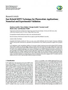
Figure 1: Spring-mass model

and solving the matrix and assuming no damping it is possible to obtain the systems effective mass (mT ) as [15]:

mT =

ω2 F = m0 + m1 2 1 2 amo (ω1 − ω )

(3)

In this equation F is the externally applied force and amo is the acceleration of the host/layer. ω1 is the resonant frequency of the spring k1 and mass m1 when attached to a rigid base and may be found using: s k1 ω1 = (4) m1 By changing the spring stiffness k1 , or internal mass m1 the resonant frequency and the amplitude may altered. The relative acceleration and phase of the the layer/host material mo and the resonator mass m1 from Figure 1 (where the supporting springs, k0 are neglected ) may be seen in Figure 2.

Theory It has been shown by Milton et al. [15], Yao et al. [16], Huang and Sun [17, 18], Gang et al.[19], Calius et al. [20] that the essential features of LRS can be captured by spring-mass models. Figure 1 is a spring-mass model representation of a single resonance LRS. This model shows a mass attached to a spring mounted on a backing layer suspended on two more springs. The point force F applied to the layer represents the pressure applied by a plane wave sound field on the structure. The response of the system shown in Figure 1 (where time dependence eiωt is assumed) can be represented as the stiffness, damping and mass matrix below:      F k0 + k1 − m0 ω 2 + iωc1 −k1 − iωc1 x0 = x1 0 −k1 − iωc1 k1 − m1 ω 2 + iωc1 F is the total force, x is the displacement, m is the mass, c is the damping coefficient and k is the spring constant. By rearranging

2

Figure 2: The logarithm acceleration of the host and resonator mass of the LRS in Figure 1 when f1 = 400Hz. The plot also shows the acceleration ratio of the resonator mass to host material It may be seen in Figure 2 and from analysis of equation 3 that ω1 at frequencies well below f1 = 2π = 400Hz, the acceleration of the host material and resonator mass is close to equal, and the effective mass is approximately the sum of the components mT = m0 + m1 . At frequencies far above the resonance frequency, where ω  ω1 , the acceleration of the resonator mass approaches zero and the total effective mass becomes the host material only, where mT = m0 . ICA 2010

Proceedings of 20th International Congress on Acoustics, ICA 2010

The frequency range most relevant to this research are frequencies around resonance. As ω approaches ω1 the resonator mass and host components are in-phase with each other. It can be seen in Figure 2 that the acceleration of the host material drops towards zero whilst the resonator mass acceleration is increasing. At ω = ω1 the ratio of the resonator mass and host acceleration is at a maximum and the host material is almost stationary. The host material has a large total effective mass and therefore sound transmission can be reflected well at this frequency.

23–27 August 2010, Sydney, Australia

(x) at an arbitrary point. The effective mass (mt ) of the system is found using the relation: F F (6) = x¨ −w2 x The effective mass per area (MT ) may then be calculated using: mT =

MT = At frequencies immediately above resonance components become out-of-phase with each other and it may be seen in Figure 2 that the acceleration of both the host and resonator mass increases to a maximum. At this point the ratio of the two components is zero. The result of this high acceleration in the host material is a decrease in the effective mass to almost zero and an increase in transmission though the structure. By substituting mT = 0 and rearranging equation 3 it can be seen that the frequency at which this occurs is described by [16]: s ω = ω1

(m0 + m) m0

(5)

The biggest draw backs found in LRS research to date are the inability to produce attenuation over a wide range of frequencies, the detrimental effects (immediately after resonance) on transmission loss from the peak acceleration of the the matrix material, and to a lesser extent, the limiting effect of damping. LRS performance, including the relative magnitude of these drawbacks, is strongly affected not only by the characteristics of the resonator itself, but more importantly by the way these local resonators are connected together to form the LRS. The realization of useful LRS-based applications depends on the combination of cost-effective materials and processes with modelling tools that enable design, analysis and optimization. A modelling-driven building block approach is being used to develop LRS designs, with experimental verification at every level. The locally resonant unit represented schematically in Figure 1 provides the basic building blocks from which groups of resonant units are integrated to form layers which are combined to form panels.

mT S

(7)

where S is the surface area of the layer/panel. Assuming θ = 0 T for normal incidence plane waves and πρfaM ca >> 1 for most well insulating walls, the sound reduction index (R0 ) of the system is then found from:   π f MT R0 = 20 log10 (8) ρa ca Transmission loss typically varies with angle of incidence. When predicting the sound reduction index for a sample subjected to diffuse field transmission (Rd ) at frequencies in the mass controlled region, equation 9 [22] was used, where R0 is plane wave simulation or experimental impedance tube sound reduction index results and k is the wavenumber. "  2 # h  1 i ω (9) Rd = R0 − 10 log10 ln kS 2 + 20 log10 1 − ω1 Three resonator configurations have been analysed using this modelling method. The first configuration is shown in Figure 1. This is a single resonance frequency system. Resonators are added to the system in parallel, but all resonators have the same resonant frequencies. Parallel configuration

The second configuration, shown in Figure 3, incorporates four resonators in parallel. Each resonator has a different frequency.

This paper presents a modelling methodology that predicts the transmission loss of a variety of resonator arrangements, together with initial measurements of sound transmission loss in an impedance tube and a full-scale room-to-room test facility. This modelling methodology is then used to explore the sensitivity of LRS performance to design parameters, with particular attention to broadening the transmission loss bandwidth and reducing detrimental effects outside this frequency band.

METHODOLOGY It is well known that complex mechanical systems can be represented by a combination of a large enough number of singledegree-of-freedom SDOF subsystems such as the one depicted schematically in Figure 1 [21]. Modelling A program ComScptv1 has been developed in Comsol script to calculate the normal incidence transmission loss of a system of layers and resonators using springs and masses coupled in various ways. The program enables the user to change the number of layers, the number of resonators per layer and the mass and spring stiffness of each component. For each springmass arrangement ComScptv1 calculates the stiffness, damping and mass matrix. ComScptv1 may then find the displacement

ICA 2010

Figure 3: Resonators in parallel. These resonators have different mass and spring stiffnesses. Damping not shown for clarity. Series configuration

The final arrangement first realised in [16] and shown in Figure 4 includes a number of resonant layers in series. Each resonator has its own mass (mr ) and spring stiffness (kr ). The resonators are attached to layers with mass (mL ). The layers are arranged in series, and separated by a inter-layer coupling spring with stiffness (kL ). In this situation any spring stiffness and mass may be altered to provide different performance characteristics. In this configuration the ComScptv1 keeps a constant system mass by changing the mass of each resonator and layer depending on the number of units in the system. Multiple high T L bands may also be created in a single structure by designing systems

3

23–27 August 2010, Sydney, Australia

Proceedings of 20th International Congress on Acoustics, ICA 2010

of layers in series with a constant inter-layer coupling spring stiffness. For example in a 9 layer system it is possible to group 3 lots of 3 layers together by changing the inter-layer coupling spring stiffness of each group to be equal.

Figure 5: Impedance tube Diffuse field testing

Figure 4: Resonators in Series. The spring stiffness, and mass of the layers are constant. All resonators have the same stiffness and mass. Damping is not shown for clarity.

Experimental methods Two different experimental methods were used to generate performance data and validate the modelling approach. Laboratory scale evaluations were performed using an impedance tube, which is suitable for testing single units or small groups of resonators, and measuring the transmission and reflection of predominantly plane waves. Full-scale measurements were performed between reverberation rooms, which were suitable for testing relatively large specimens consisting of many resonators under diffuse sound field conditions.

The room-to-room testing facility shown in Figure 6 used for full-scale diffuse field testing was designed to ISO 140-3. Two reverberation rooms (202 and 208 m3 ) are used to measure the sound reduction index of the samples. The test specimen is placed so as to fill the adjustable gap between two well-insulated sliding doors that separate the two rooms. A broadband pink noise source signal is then placed in one of the rooms. The spatial average sound pressure and reverberation times RT in the emitting and receiving rooms is then measured using 1/2“ B&K 4190 and 4165 microphone. The process is then repeated with the noise source in the other room. Data was processed in third octaves.

Plane wave testing

The impedance tube was adapted for normal incidence transmission loss measurements and designed to conform to the European Standard ISO 10534-2:2001(E). The dimensions of the tube shown in Figure 5 are based around the B & K Type 4026 impedance tube. The resonator units being tested were housed within a 100mm diameter hollow cylinder made from medium density fibre MDF, which could contain several resonators. Alternative resonator designs were attached to a backing plate that represented the matrix material of the LRS. The cylindrical LRS sample was suspended on two rubber rings between two parts of the impedance tube. A loud speaker generates plane wave sound that propagates down the first tube. Part of the signal is transmitted through the sample which is measured in the second tube using three microphones. Microphones 1, 2 and 3 are used to find the transmitted side complex wave constants A and B whilst microphones 4, 5 and 6 are used to find the receiving complex wave constants C and D. The pressures found from each B&K 4190 microphone may be written as the equations shown below: P1 = Ae j(ωt−kx1 ) + Be j(ωt+kx1 ) P2 = Ae j(ωt−kx2 ) + Be j(ωt+kx2 ) P3 = Ae j(ωt−kx3 ) + Be j(ωt+kx3 ) P4 = Ce j(ωt−kx4 ) + De j(ωt+kx4 ) P5 = Ce j(ωt−kx5 ) + De j(ωt+kx5 ) P6 = Ce j(ωt−kx6 ) + De j(ωt+kx6 ) The constants (A,B,C,D) are then found by solving the complex equations using the least squares determinant method. The receiving side of the impedance tube is in anechoic conditions where reflections (D) are assumed to be near 0 and hence the transmission coefficient is found to be near the ratio of A to AC−BD C. The transfer coefficient may be found from τ = AA−DD Where τ is the transmission coefficient. When τ is applied to R = 20 log10 (1/|τ|) the sound reduction index may be found. 4

Figure 6: The University of Auckland acoustic research centre (ARC) room to room testing facility.

In order to study the frequency response in more detail than 3rd octaves, the spectrum was found by calculating the Power spectral density (square of the magnitude of the Fourier transform of the signal) from the raw time domain pressure signals. The narrow band RT was found by interpolating the 3rd octave RT results. The absorption area of the receiving room was found using: 0.163V A= (10) T60 where T60 is the reverberation time, V is the volume of the receiving room. The level difference (δ L) of the specimen was then calculated from: δ L = 10 log10 [P0 ] − 10 log10 [P1 ]

(11)

where P0 is the incident sound power and P1 is the radiated sound power. Under the assumption of diffuse sound fields in the transmitting and receiving rooms the actual sound reduction index of the specimen may be found using:   S Rd = δ L + 10 log10 (12) A where S is the area of the wall specimen. The single-layer panel consisted of 252 resonators attached to a 2.65 x 0.95 x 0.01m plasterboard matrix layer using Loctite 401 adhesive.

ICA 2010

Proceedings of 20th International Congress on Acoustics, ICA 2010

23–27 August 2010, Sydney, Australia

The accelerations perpendicular to the panel plane were also measured while the panel was subjected to pink noise . For each measurement two PCB A353 B65 accelerometers were attached at any 2 of 9 different positions on the back of the panel using wax. As well as the amplitude of the acceleration as a function of frequency at various locations, these measurements also allowed the phase difference to be calculated between adjacent resonators. This testing method gives in-site into the sound insulating performance of large scale meta-material samples under a diffuse field.

RESULTS Single frequency locally resonant structures The features of a single frequency LRS have been modelled and are shown in Figure 7. There is a large increase in transmission loss at 400Hz which occurs at the resonant frequency (ω1 ) of the resonator. At this frequency the host material has its lowest acceleration magnitude and the LRS has a high effective mass. ω1 may be manipulated by changing the mass and stiffness of the resonator spring and mass. The large dip in transmission loss soon after this peak is the result of a high acceleration magnitude of both the host and resonator mass and therefore a low total effective mass. The effect of damping in a single resonant frequency arrangement is also shown in Figure 7. It can be seen that as damping is increased there is a smoothing effect on the resonant peak. Higher damping lowers the maximum peak sound reduction index, but also reduces the sound reduction index dip.

Figure 8: Frequency comparisons of diffuse field transmission loss and typical panel acceleration for a large single resonant frequency LRS panel.

are also transmission loss performance benefits. These are indicated by the shaded region in Figure 7. If ω1 is raised in frequency (by increasing the spring stiffness), both the sound reduction index performance gains over mass law and frequency band width increases. Parallel multi frequency systems The results of parallel arrangements of non-identical resonators on a single layer are presented in this section. The predicted and measured plane wave sound transmission loss for an LRS with four non-identical resonator units arranged in parallel configuration similar to Figure 3 are compared in Figure 9. The LRS consisted of four individual resonators spaced at resonant frequencies of 40Hz apart, each with equal mass, but differing in spring stiffness. The results from impedance tube testing provide experimental verification of the spring mass model, with excellent agreement near the resonant region and above. The resonance of the compliant rubber suspension system that holds the LRS test specimen in the impedance tube is responsible for the additional transmission loss peak and valley observed in the test data below 200 Hz.

Figure 7: Comparison of transmission loss verse frequency of a single resonant frequency LRS showing the effect of increasing the damping factor ζ from 0.001 to 0.1. The results for a single-layer panel with 252 nominally identical resonators arranged in a system essentially like Figure 1 are given in Figure 8. The top graph shows the experimental transmission loss obtained from full-scale testing of the panel and the transmission loss for the equivalent diffuse field spring mass model over the frequency range of interest approximated by equation 9. It is clear that there is a good match between the model and experiment above 200 Hz. At frequencies below 200 Hz the uncertainty in the measurements increases significantly as the wavelength starts to approach the panel and reverberant room dimensions and the panel mounting resonance is reached. This effect rapidly escalates at 100 Hz and below. The bottom graph gives the acceleration of the panel at its centre over the same frequency range. This graph confirms the acceleration of the host/panel material is at a minimum when the transmission loss is at a maximum and visa-versa. It has been observed from single resonance modelling and experimental analysis that not only is there a transmission loss performance gain at around ω1 , but before this frequency there ICA 2010

Figure 9: Comparison of transmission loss verses frequency of modelling and experimental results for a LRS with four nonidentical resonator units arranged in parallel. The host mass law is also shown. Figure 10 shows the sound reduction index results when modelling 15 resonators in parallel. All 15 masses are of equal weight, but their frequency of resonance is defined by the spring stiffness of the resonator. The resonant frequencies have been spaced 15 Hz apart, and a small amount of damping ζ = 0.01 has been added to create a more realistic representation of the

5

23–27 August 2010, Sydney, Australia

material. Also included in this plot is a single resonator with the total mass of the sum of all 15 resonators with the same damping factor. The mass law of the host material and total system is also shown. It can be seen that the parallel arrangement approximately doubles the bandwidth of attenuation above mass law with some reduction in T L.

Figure 10: Comparison of single frequency and 15 frequencies LRS. The latter has 15 resonant frequencies generated by resonators arranged in parallel. The total system mass is constant with a damping factor ζ = 0.01 The sound transmission loss for a LRS with 8 different resonators is shown in Figure 11. Note the damping factor of ζ = 0.05 is significantly higher than for the similar system whose response is given in Figure 10. The plot also shows a more gradual reduction in transmission loss that avoids the development of a dip in transmission loss around 950Hz. This is due to the use of mass tail-off where the mass of the highest frequency resonator is lowered from 0.03 to 0.004 relative to the lowest. A table of the relevant variables for the resonators are shown in table 1.

Figure 11: Comparison of transmission loss verses frequency for parallel LRS with equal mass resonators and tapered mass resonators. Damping ζ = 0.05 is used.

Proceedings of 20th International Congress on Acoustics, ICA 2010

the band gap increases in attenuation, however the width of this region remains similar. With an increase in the number of layers there is an increase in the number of transmission loss dips before and after the band gap.

Figure 12: Comparison of transmission loss verses frequency for 2 and 10 layer LRS. Inter-layer coupling spring and resonator spring stiffnesses are all constant and a damping factor ζ of 0.001 is used. Figure 13 shows sound transmission loss of a three layer system with variation in the inter-layer coupling spring stiffness, kL . As kL is reduced, while the spring stiffness of the resonators, kr remains constant, the frequency band width of high attenuation increases by a factor of 3 while the peak attenuation remains constant. The band width is dictated by the ratio of kL to kr and kL must be lower than kr for a wide attenuation band to occur.

Figure 13: Comparison of transmission loss verses frequency of a 3 layer LRS. The frequency of resonance of the resonators (fr) remains constant while the inter-layer coupling frequencies of resonance (fl) are tuned to resonant frequencies from 400800Hz by adjusting kL . The model uses a damping factor ζ of 0.001.

Series systems Systems consisting of series-coupled resonators are investigated in this section. The predicted transmission loss for seriescoupled systems are shown in Figures 12-15. Figure 12 shows the predicted transmission loss for a multilayer system similar to Figure 4. The plot shows the sound reduction index as a function of frequency for increasing numbers of layers. The total mass of the system is held constant as the number of layers is increased. A low damping factor of 0.001 is applied throughout the arrangement. There is high attenuation present between approximately 400 and 500Hz. As the number of layers increases

6

A three layer system with the addition of damping is shown in Figure 14. High damping was applied (ζ = 0.1) to the interlayer coupling springs. Damping in the resonator springs remained low(ζ = 0.001). Transmission loss dips before and after the band of high T L are significantly reduced without effecting the high T L band magnitude. An example of a system with multiple band gaps is shown in Figure 15. This system consists of a total of 9 layers created by coupling 3 groups of 3 layers. The inter-layer coupling

ICA 2010

Proceedings of 20th International Congress on Acoustics, ICA 2010

23–27 August 2010, Sydney, Australia

Table 1: Table of resonator variables Frequency(Hz)

400

450

510

580

670

770

890

1010

Mass(kg)

0.03

0.027

0.023

0.019

0.014

0.01

0.007

0.004

Damping(ζ )

0.0464

0.0458

0.0475

0.0505

0.0594

0.0723

0.0894

0.1379

Figure 14: Comparison of the effect damping in the inter-layer coupling springs has on transmission loss verses frequency of a 3 layer LRS. The damping factor ζ in the inter-layer coupling springs ranges from 0.001 to 0.1.

springs in each group are tuned to the same resonant frequency fl and resonators in each group are tuned to the same resonant frequency fr. For the first group f1=400Hz and fr=500Hz, for the second group f1=800Hz and fr=900Hz and for the last group f1=1200Hz and fr=1300Hz.

Figure 16: Comparison of transmission loss verses frequency of a 15 layer LRS. As the layer number increase so does the frequency of resonance of the resonators. Resonators are tuned at increments of 15Hz by changing the resonator spring stiffness. The inter-layer coupling spring stiffness remains constant throughout the system. A damping factor ζ of 0.001 is used.

layer has the individual performance shown in Figure 10. When the layers are combined in series with a constant inter-layer coupling spring stiffness, there is an increase in transmission loss over the equivalent single layer parallel arrangement for the same frequency range (between 400 and 650Hz).

Figure 15: Comparison of transmission loss verses frequency for a 9 layer multi-band-gap LRS. 3 layer groups tuned at 3 different frequencies. There is a damping factor ζ of 0.001 and 0.1 in the inter-layer coupling springs.

Series Parallel systems Series and parallel arrangements may be combined to incorporate their different performance characteristics. Figure 16 shows the performance of a 15 layer system. The inter-layer coupling spring stiffnesses are constant throughout the system. The resonator resonant frequency increases with layer number in increments of 15Hz via changing the resonator spring stiffness. The band of large transmission loss has been widened to between approximately 400 and 650Hz compared with 400 and 500Hz for the conventional 10 layer series system shown in 12 with the same total system mass. Figure 17 shows 8 layers of parallel arranged resonators in series. There are 15 parallel resonators on each layer. Each

ICA 2010

Figure 17: Comparison of transmission loss verses frequency of a 8 layer LRS with 15 parallel resonators on each layer. The parallel resonators on each layer are tuned at incremental resonant frequencies of 15Hz while the inter-layer coupling spring stiffness remains constant throughout the system. A damping factor ζ = 0.1 in the resonators is used.

DISCUSSION The results obtained for single-frequency LRS through both experimental observations and analysis indicates that when ω