Modelling cohesive interfaces with a regularized XFEM formulation Elena Benvenuti ENDIF Universit`a di Ferrara, via Saragat 1, I-44100 Ferrara E-mail:
[email protected] Keywords: xfem, discontinuous displacement, regularization, cohesive models. SUMMARY. A continuum two-fields extended finite element formulation enriched with a regularization length is presented. By extending the mechanical framework for elastic interfaces proposed in [Benvenuti et al. 2007], the geometrical discontinuity is replaced by a regularized layer with an elastodamaging behavior. Salient features of the proposed methodology are that a continuum cohesive-like stress field and a “bridging” stress field emerge, while the cohesive traction-separation work is proved to be recovered when the regularization length vanishes. 1 INTRODUCTION Interfaces with finite or zero thickness are of great interest in engineering applications as they can imply structural failure. In this work, interfaces characterized by the presence of displacement discontinuities are considered. A soft and thin layer is embedded in a body, and modelled as an elastodamaging material. Its thickness introduces a characteristic length scale into the continuum model. When the characteristic length vanishes, an interface governed by a cohesive traction-separation law is recovered. In particular, the displacement and the regularized jump are approximated through the finite element interpolation function as independent fields. The associated finite element formulation satisfies the local Partition of Unity property of standard finite element interpolation functions, and it can be seen as an “eXtended Finite Element” formulation [Moes et al. 1999] based on a regularized kinematics. A peculiarity of this work is the constitutive modelling of the stresses which are workconjugated to the strain components: the “standard” stress, the stress associated to the jump, and, finally, the stress localized in the regularized layer. In particular, following Hashin (1990), the latter is modelled as a spring-like stress obeying an elastodamaging constitutive law, which converges to a cohesive traction-opening law as ρ vanishes. An earlier study of the most appropriate quadrature techniques has shown that the adopted approach can avoid the use of integration subdomains, which is usual in standard XFEM models [Benvenuti et al. 2007]. To the purpose of illustrating the links of the model with standard cohesive models, finite element results concerning deadhesion in DCB tests are shown. 2 THE PROBLEM Let us focus attention on a simplified problem: a body Ω in Rn (n = 2, 3) with smooth boundary ¯ on ∂Ωu and to given surface load distribution p ¯ on ∂Ω, subjected to prescribed displacements u = u ∂Ωp (Figure 1a). Volume forces f in Ω are also included. Let the domain be divided by a, planar for the sake of simplicity, internal surface ∂Ωd parallel to the coordinate plane x1 , x2 into two disjoint zones, across which the displacement u exhibits a bounded jump to which the vector field ( [[u]](x) = u+ (x) − u− (x) x ∈ ∂Ωd a(x) = (1) 0 otherwise is associated, which is assumed sufficiently continuous and bounded. Moreover, u+ and u− denote the values of the displacement field across the discontinuity surface. At a point x ∈ Ω, let the 1
+
+
Ω Ωd − Ω
p
p
n
x1
n
2Lρ
x3
u
Ω Ωρ − Ω x3
u
x2
x1
x2
Figure 1: Domain Ω in the R3 space: non regularized discontinuity surface ∂Ωd (left) and regularized layer Ωρ of thickness 2Lρ (right) .
scalar signed distance function d(x) be defined as d(x) := |¯ x − x| if (¯ x − x) · n(x) ≥ 0 and ¯ is the closest point projection of x onto Ωd . d(x) := −|¯ x − x| if (¯ x − x) · n(x) < 0, where x Given the Heaviside (step) function H, that is such that H(d(x)) = 1 if d(x) ≥ 0, and H(x) = 0 if d(x) < 0, the displacement field can be expressed as u = v + Ha
(2)
A regularized approximation Hρ (x) of H is considered, such as, for instance, Hρ (d(x)) =
1 Vρ (x)
Z
d(x)
e
−
|ξ|2 ρ2
dξ
(3)
−∞
√ where |ξ| denotes the absolute value of ξ and Vρ = (ρ 2π)n in Rn . An alternative expression is [Benvenuti et al. 2007] Hρ (d(x)) =
1 Vρ
Z
d(x)
e−
|ξ| ρ
dξ = sign(d(x))(1 − e−
|d(x)| ρ
))
(4)
0
A pictorial representation of Hρ and its derivative ∇Hρ = δρ in the one-dimensional case is displayed in Figure 2 for the case of function (4) by adopting various values of the parameter ρ, namely ρ = 0.01, 0.02, 0.03, 0.04 mm. Other choices are available; for instance, in the XFEM analysis [Patz´ak and M. Jir´asek 2003] the piecewise polynomial bell function was used. The displacement field is written as uρ = v + Hρ a (5) The discontinuity surface ∂Ωd results being replaced with a layer of finite thickness 2Lρ (Lρ ∈ R): the model adhesive layer. The parameter ρ will be referred to as the regularization parameter, while the layer of width 2Lρ will be hereafter denoted the regularization layer Ωρ . Finally , the domain turns out being divided into three disjoint parts: Ω+ ,Ωρ , and Ω− . An explicative picture is given in Figure 1, where the discontinuity surface develops in the plane x1 , x3 , while x2 denotes the direction along which the regularization is carried out. Moreover, it is trivial to verify that, for vanishing ρ, 2
the displacement field assumes the following expression limρ→0 uρ = v(x) + H(x)a(x), i.e. the displacement is the superposition of a continuous displacement and a discontinuous displacement. The discrete form of the problem is next synthetically considered, more details can be found in [Simo and Hughes 1998]. Let us consider a loading history within the interval of interest τ = [0, T ], and discretize this interval into N nonoverlapping intervals. Let the solution of the equilibrium problem at the instant told be known. After the load change during the time step [told , t], the updated solution at t is obtained according to the Backward Euler scheme. Domain discretization SM is achieved by approximating the domain Ω through M non over-lapping finite elements Ω ≡ i=1 Ωi connected at N nodes. The primal fields v and a are approximated over the set of the N nodal values vI , aI through the same polynomial shape functions NI , I = 1, · · · , N . Let the vectors V = {v1 , v2 , . . . , vN } and A = {a1 , a2 , . . . , aN } collect the N nodal values, and let N = {N1 , N2 , . . . , NN } collect the N nodal shape functions v ≈ NVa ≈ NA. The approximated displacement field u yields the following expression uρ = NV + Hρ NA
(6)
which satisfies the local Partition of Unity property of standard finite element shape functions. The present formulation can thus be seen as a special type of extended finite element formulation. Let V and A be the space of the admissible fields v and a, such that v ∈ V satisfies the Dirichlet ¯ in ∂Ωu , and a = 0 in ∂Ωu . Let us assume virtual variations v ˜ and a ˜ that satisfy conditions v = u homogeneous boundary conditions.
Hρ
1
100
0.8
90
δρ
0.6 0.4
ρ=0.01 ρ=0.02 ρ=0.03 ρ=0.04
0.2 0
70 60 50
−0.2
40
−0.4
30
−0.6
20 10
−0.8 −1
ρ=0.01 ρ=0.02 ρ=0.03 ρ=0.04
80
−0.2
−0.1
0
0.1
0.2
0
0.3
−0.2
−0.1
0
d(x)
0.1
0.2
0.3
d(x)
Figure 2: One-dimensional spatial representation of function Hρ (4) and its derivative δρ for ρ = 0.01, 0.02, 0.03, 0.04.
In this work, infinitesimal strain and displacement fields are considered; an extension to finite elasticity is possible. The strain field associated to the displacement field (6) is ερ = ∇uρ = B1 V + Hρ B2 A + δρ B3 A
(7)
where the symmetric compatibility operators ¯ B1 = LN , B2 = B1 ∇N , B3 = NN where δρ := |∇Hρ | =
∂Hρ ∂ d ∇d
= |δρ n| and nx 0 ¯ t = 0 ny N 0 0
0 0 nz 3
ny nx 0
0 nz ny
nz 0 nx
(8)
(9)
and the matrix L is
L=
∂ ∂x1
0
0 0
∂ ∂x2
∂ ∂x2
∂ ∂x1 ∂ ∂x3
0
∂ ∂x3
0
0
0 0 ∂ ∂x3
0
∂ ∂x2 ∂ ∂x1
(10)
2.1 Free energy potential Therefore, the strain field turns out being the sum of the following functions: ε1 := B1 V , ε2ρ := Hρ B2 A , ε3ρ := δρ B3 A
(11a)
The different mathematical structure of the strain fields (11a) reflects the fact that each strain term is the expression of a particular mechanical aspect. For instance, ε1 is the strain the body would undergo in the absence of the discontinuity. The strain ε2ρ is associated to the spatial gradient of the jump a and is defined over the entire body Ω. The strain field ε3ρ is different from zero at Ωρ and vanishes outside, as it is proportional to the spatial gradient δρ . Owing to its structure, see for instance [Suquet 1987], ε3ρ is a localization strain precursor of the interfacial displacement discontinuity. Let us consider the following free energy density function ψ(ε1 , ε2ρ , ε3ρ , d) = ψ 1 (ε1 ) + ψρ2 (ε2ρ ) + ψρ3 (ε3ρ , d, ξ)
(12)
where it is assumed that ψρ3 is of elastodamaging type and depends on the hardening internal variable ξ, and the isotropic damage scalar d ranging from 0 to 1 [Benvenuti et al. 2002]. Inelasticity is hence restricted to the energy ψ 3 , only. In particular, the potential density ψ 1 is assumed as the quadratic function 1 ψ 1 = ε1 · D1 ε1 (13) 2 where D1 is the elasticity constitutive operator associated to the “bulk” mechanical behavior. The free energies ψρ2 (ε2ρ ) and ψρ3 (ε3ρ , d, ξ) that are associated to the strain fields ε2ρ and ε3ρ are defined as 1 1 ¯ 3 ε3 + 1 h ξ 2 ψρ2 = ε2ρ · D2 ε2ρ , ψρ3 = f (d) ε3ρ · D (14) ρ 2 2 2 where f (d) is a damage function. In Equations (14), two constitutive tensors have been introduced, ¯ 3 , and the hardening scalar parameter h. This choice is quite general, as it is supposed D2 and D that the energy associated to the strain fields ε2ρ and ε3ρ can be seen as the expression of different mechanical phenomena. The set of the state laws σ1 =
∂ψρ2 ∂ψρ3 ∂ψ 1 ¯ 3 ε3 = D1 ε1 , σ 2ρ = = Hρ D2 ε2ρ , σ 3ρ = f (d) 3 = f (d) D ρ 1 2 ∂ε ∂ερ ∂ερ
Yρ3 = −
∂ψρ3 ∂ψρ3 1 ∂f (d) 3 ¯ 3 3 =− ερ · D ερ , X 3 = = hξ ∂d 2 ∂d ∂ξ
(15a) (15b)
¯ 3 is the constitutive matrix of the sound can be deduced from the above energy functions, where D 1 2 3 elastic material. The stress fields σ , σ ρ and σ ρ emerge as energy-conjugated to the homologous 4
strain fields. The thermodynamic forces Yρ3 are conjugated to the damage state variable d and to the hardening variable ξ, respectively. 2.2 Elasto-damaging constitutive law As it can be drawn from the definition of ψρ3 , a basic ingredient is the introduction of an equivalent material in Ωρ , that has an elastodamaging behavior: when the damaging process has not been ¯ 3 , which can be seen as the tensor activated, the material is characterized by an elasticity tensor D collecting the “homogenized” elastic constants of the inhomogeneous material of the layer. The function f (d) of the isotropic damage scalar d makes it possible to achieve an elasto-damaging stress-strain law. The stress field σ 3ρ is a volume field, i.e. it is defined at each point of the volume Ωρ . Thus its traction component T = σ 3ρ n cannot be identified as an interfacial traction in a strict sense. For this reason, it is next investigated whether and in which conditions a standard traction separation law of the same type as described above may be recovered in the limit case of vanishing ρ. ˆ 3 and µ Let λ ˆ3 be the constitutive parameters of the adhesive layer. The following equivalent elastic moduli are considered ¯ 3 (x) = λ
ˆ3 λ λ3 = , tδρ (x) δρ (x)
µ ¯3 (x) =
µ ˆ3 µ3 = tδρ (x) δρ (x)
(16)
where the characteristic length t is often assumed to coincide with the adhesive thickness ( [Hashin 1990] [Allix and Corigliano 1999]). Therefore, the constitutive tensor yields ¯ 3 (x) = D
D3 D3 = tδρ (x) δρ (x)
(17)
The choice (17) is dictated by the necessity of having a bounded stress field within the regularization layer, as it will be shown in the following developments. After replacement of Equation (17), the expression of the potential ψρ3 becomes ψρ3 =
1 f (d)δρ (a ⊗s n) · D3 (a ⊗s n) 2
(18)
A detailed investigation of the type of constitutive laws that are best appropriate to describe the complex behavior of adhesive interface is out of the aims of the present work. For the sake of simplicity, the function f (d) is assumed to be a quadratic function of s. Hence, the state laws σ 3ρ = f (d)D3 (a ⊗s n) , Yρ3 = −
1 ∂f (d) δρ (a ⊗s n) · D3 (a ⊗s n) 2 ∂d
(19)
define the relevant constitutive laws. 2.3 Interfacial damage evolution The adhesive layer is usually a heterogeneous material, whose deformative behavior is complex: first early micro-cracks arise and eventually coalesce into macroscopic cracks with consequent unloading of the surrounding region. Experimental results prove that, at the structural scale, the mechanical behavior of the adhesive layer can be modelled by introducing within the description a cohesive surface whose traction-separation law is characterized by an elastic linear branch up to a peak followed by a softening branch [Andersson and Biel 2006]. 5
The quadratic elastodamaging constitutive law σ 3ρ = (1 − d)2 D3 ε3ρ
(20)
is adopted, that has been previously proposed in a thermodynamically consistent formulation for non-local damage [Benvenuti et al. 2002]. Let us introduce a damage activation function φ as a function of the thermodynamic forces Yρ3 and X 3 thermodynamically conjugated to d and ξ φ(Yρ3 , X 3 ) ≤ 0
(21)
If associative damage is assumed, then the usual laws for generalized standard materials are [Lemaitre and Chaboche 1990] ∂φ ∂φ d˙ = γ˙ , ξ˙ = γ˙ , φ(Yρ3 , X 3 ) ≤ 0 , 3 ∂Yρ ∂X 3
γ˙ ≥ 0 , φγ˙ = 0
(22)
The simplest possible form of the damage activation function is the bilinear function φ(Yρ3 , X 3 ) = Yρ3 − X 3 − Y0 ≤ 0
(23)
which implies the following loading-unloading conditions: d˙ = γ˙ ,
ξ˙ = γ˙ ,
φ(Yρ3 , X 3 ) ≤ 0 ,
γ˙ ≥ 0 , φγ˙ = 0
(24)
The response to a given increment ε˙3 ρ at the points x in the part of Ωρ where damage is active is obtained by solving the following set of loading-unloading conditions ˙ 3 , X 3 ) = Y˙ 3 − hd˙ ≤ 0 , d˙ ≥ 0 , φ˙ d˙ = 0 φ(Y ρ ρ
(25)
In the present formulation, the following set of constitutive equalities and inequalities is used: σ 3ρ = (1 − d)2 D3 ε3ρ , Yρ3 = (1 − d)ε3ρ · D3 ε3ρ φ = Y 3 − Y0 − hd ≤ 0 , d˙ ≥ 0 , φ d˙ = 0 ρ
(26a) (26b)
The relevant material parameters are the threshold Y0 , the hardening parameter h and the regularization length ρ. When the regularization layer vanishes, the resulting normalized tractionseparation law is shown in Figure 3, where it is evident that the same constitutive law for Tn and Tt was assumed. This a simplification that can be however overcome without modifying the essence of the approach. It is worth noting that, despite its simplicity, the current constitutive model is close to the traction separation laws that were experimentally measured in References [Andersson and Biel 2006]. Alfano has in particular shown that, in the simple case of a DCB test, the shape of the adopted law does not significantly influence the structural response in terms of load versus the crack opening displacement if the same stress peak value and the same fracture energy are adopted [Alfano 2006]. 2.4 Principle of virtual work ˜ and a ˜ Let σ 1 , σ 2ρ , σ 3ρ be the stress fields characterizing the body in equilibrium, and consider v virtual admissible fields satisfying the Dirichlet boundary conditions. ˜1 = ∇˜ The internal virtual work W int that the system will spend for the virtual strains ε v, 3 2 ˜ρ = δρ (˜ ˜ρ = Hρ ∇˜ a ⊗s n) is postulated in the following form a, ε ε Z Z ˜3ρ dΩ ˜) = (σ 1 + σ 2ρ ) · (˜ ˜2ρ ) dΩ + (27) σ 3ρ · ε W int (˜ v, a ε1 + ε Ωρ
Ω
6
T¯n , T¯t
1
h↑
0
0
0.2
0.4
0.6
0.8
1
an , at Figure 3: Normalized one-dimensional traction-separation relationships for increasing values of the constitutive parameter h, h = 0.1, 1, 5, 10. where it has been assumed mechanical uncoupling between σ 1 + σ 2ρ and ε3ρ and between σ 3ρ and ε1 + ε2ρ . The principle of virtual work states the equality between the virtual internal work and the virtual external work Z Z Z Z 1 2 3 1 2 3 ˜ρ ) dΩ + ˜ρ dΩ = ˜) dΩ + ˜ dS (28) (σ + σ ρ ) · (˜ ε +ε σρ · ε F · (˜ v + Hρ a p·v Ω
Ωρ
∂Ωp
Ω
˜, a ˜ . The discrete form of the principle of virtual power for any virtual v Z ˜ + Hρ B2 A) ˜ dΩ+ (D1 B1 V + Hρ D2 B2 A) · (B1 V ZΩ
Z
t
δρ f (d)At B3 · D3 B3 A dΩ = Ωρ
NF · V dS
(29)
∂Ωf
˜ and A, ˜ that defines the set of the solving equations equations, holds for any admissible variation V under the loading-unloading conditions (31). Therefore, the problem to be solved is: Find V and A such that Z Z t t LV = B1 D1 B1 V + B2 D2 B2 Hρ A dΩ − Nt F dΩ = 0 (30a) Ω Ω Z Z t t t LA = Hρ B2 D2 B1 V + Hρ2 B2 D1 B2 A dΩ + δρ f (d) B3 D3 B3 A dΩ = 0 (30b) Ω
Ωρ
where the loading-unloading conditions t
σ 3ρ n = f (dn )D3 B3 An , f (dn ) = (1 − dn )2 , Yρ3 = (1 − d)δρ At B3 D3 B3 A
(31a)
φ = Yρ3 − Y0 − h d ≤ 0 ∆ d ≥ 0 , ∆dφ = 0
(31b)
7
hold. As the solving equations are non-linear in V, A, a Newton-Raphson linearization procedure is carried out. At the equilibrium iteration i within the load step n, the variables are written in the iterative form Vi = Vi−1 + δVi , Ai = Ai−1 + δAi (32) where the variations (δVi , δAi ) are calculated by solving the equilibrium equations ·
KVV KAV
KVA KAA
¸i−1 ·
δV δA
·
¸i =
−LV −LA
¸i−1
The components of the tangent stiffness matrix Ki−1 write Z Z t t B1 D2 B2 Hρ dΩ B1 D1 B1 dΩ , KVA = KVV = Ω ZΩ Z Z t 2 1 2 2 2t 2 2 KAV = Hρ B D B dΩ , KAA = Hρ B D B dΩ + Ω
Ω
(33)
(34a) t
δρ f (d) B3 D3 B3 dΩ Ωρ
(34b) Note that, generally, the stiffness matrix is symmetric only when D1 = D2 . 2.5 Limit case for vanishing ρ Let us consider the limit case of the formulation when ρ becomes smaller and smaller, namely smaller than the minimal distance allowed from the adopted mesh of quadrature points. It can be proved that [Benvenuti et al. 2007] Z Z (35) lim σ 3ρ n · [[u]] dS σ 3ρ · ερ3 dV = ρ→0
∂Ωd
Ωρ
That means that the traction-separation work can be recovered for decreasing values of ρ. In this case, the problem becomes: Find v and a such that, for D1 = D2 Z Z t t (B1 D1 B1 v + B1 D1 B2 Ha) dΩ = Nt F dΩ Ω ZΩ 2t 1 1 2 2t 1 2 (HB D B v + H B D B a) dΩ = 0
(36a) (36b)
Ω
R t The component Kaa becomes Kaa = Ω H2 B3 D2 B3 dΩ. It is worth noting that Equations (36) are the algebraic expression of standard extended finite element formulation for strong discontinuity for vanishing ρ, e.g. [Moes and Belytschko 2002] [Moes et al. 1999]. In order for the current approach to be consistent with the standard XFEM formulations when the regularization length vanishes, D1 = D2 must be assumed. 3 EXAMPLE The experimental simulations of delamination in composite laminates described in Reference [Robinson and Song 1991] are considered. A DCB specimen of length L = 100 mm, width W = 30 8
P/W[N/mm]
4 exp set 1 set 2 anal
3.5 3 2.5 2 1.5 1 0.5 0 0
2
4
6
8
10
I
δ [mm] Figure 4: DCB test: load per unit thickness versus crack opening displacement obtained by adopting Y0 =1.3 , h=0.1, E ad =126000/15 N/mm3 , comparison of the results for ρ = 0.008mm and the experimental and analytical results. mm, initial opening a0 = 30mm are compared with the computational response. The material is unidirectional carbon fibre epoxy composite with E11 = 126000 Mpa and ν = 0.263. The load per unit thickness curves versus the opening displacement δ I are displayed in Figure 4; they have been obtained by setting ρ = 0.008mm, Y0 = 1.3 N/mm2 , h = 0.1 and by adopting various values of the adhesive stiffness. The continuous line is the present numerical response while the cross markers denote the experimental results reported in Reference [Robinson and Song 1991]. The adhesive layer was given a Fracture Energy GI = 0.281 N/mm. The results were compared with the beam analytical solution 2 (W EGI J)3/2 δI = (37) 3 E J P2 In the previous results, the stiffness D2 was set equal to D1 , namely a symmetric stiffness matrix was used. The stiffness D2 is related to the stress field σ 2ρ , whose effect is worth being investigated. For instance, in Figure (5), the profiles obtained by experiencing different values of the stiffness D2 are reported. They show that the stress field σ 2ρ influences the peak value and the energy dissipation of the model. More precisely, it can be deduced that a bridging effect which increases for increasing values of the elastic constants corresponding to D2 emerges. 4 CONCLUSIONS A regularized finite element formulation based on the extended finite element method has been presented. Attention was restricted to assess the merits and limits of the approach for a simple class of problems, namely modelling of deadhesion of composite beams along adhesive layers. The numerical tests have pointed out the links of the model with standard discrete cohesive models. References [Alfano 2006] G.Alfano. On the influence of the shape of the interface law on the application of cohesive-zone models, Composites Science and Technology 66 (2006) 723730.
9
P/W[N/mm]
4 3.5 3 2.5 2 1.5 E2=E1*2 E2=E1 E2=E1/10
1 0.5 0 0
1
2
3
4
5
6
7
8
I
δ [mm] Figure 5: DCB test: load per unit thickness versus crack opening displacement obtained by adopting Y0 =1.3 , h=0.1, ρ = 0.008 mm: comparison of the results obtained with different values of the adhesive Young modulus E 2 , while E 1 denotes the Young modulus of the adherends. [Andersson and Biel 2006] T.Andersson, A.Biel. On the effective constitutive properties of a thin adhesive layer loaded in peel. International Journal of Fracture, 2006; 141: 227-246. [Allix and Corigliano 1999] O. Allix, A.Corigliano. Geometrical and interfacial non-linearities in the analysis of delamination in composites. International Journal of Solids and Structures, 1999; 36: 2189–2216. [Benvenuti et al. 2002] E. Benvenuti,G. Borino,A. Tralli. A thermodynamically consistent nonlocal model for elasto-damaging materials. European Journal of Mechanics A/Solids 2002; 21:535-553. [Benvenuti et al. 2007] E.Benvenuti, A.Tralli, G.Ventura, A regularized XFEM model for the transition from continuous to discontinuous displacements, 2007, submitted. [Hashin 1990] Z. Hashin, 1990. Thermoelastic properties and conductivity of carbon/carbon fiber composites, Mechanics of Materials, 8, 293-308. [Lemaitre and Chaboche 1990] J.Lemaitre, J.L.Chaboche, Mechanics of Solids, Cambridge University Press (1990). [Moes et al. 1999] N. Moes, Dolbow J, T. Belytschko. A finite element method for crack growth without remeshing. International Journal for Numerical Methods in Engineering 1999; 46, 131–150. [Moes and Belytschko 2002] N. Moes, T. Belytschko. Extended finite element method for cohesive crack growth. Engineering Fracture Mechanics 2002; 69:813-833. [Patz´ak and M. Jir´asek 2003] B. Patz´ak, M. Jir´asek. Process zone resolution by extended finite elements. Engineering Fracture Mechanics 2003;70: 957 977. [Robinson and Song 1991] P.Robinson, DQ.Song. A modified DCB Specimen for Mode I testing of Multidirectional Laminates, Journal of Composite Materials, 1991; 26: 1554–1577. [Simo and Hughes 1998] J. Simo, T. Hughes, Computational inelasticity. Springer Verlag, New York, 1998. [Suquet 1987] P. Suquet, 1987. Discontinuities and plasticity. In: JJ.Moreau,PD. Panagiotopoulos Eds., Nonsmooth Mechanics and applications, Springer Verlag, Berlin, 280–340.
10
Modelling cohesive interfaces with a regularized XFEM formulation Elena Benvenuti Dipartimento di Ingegneria, Universit`a di Ferrara, via Saragat, 1- 44100 Ferrara
[email protected], ph. 0532 974935 fax 974870 Keywords: xfem, discontinuous displacement, regularization, cohesive models. Interfaces with finite or zero thickness are of great interest in structural mechanics applications. In this work, a soft and thin layer is embedded in a body and the corresponding finite element scheme is presented. The process zone is modelled as a soft elastodamaging layer, whose thickness introduces a characteristic length scale into the continuum model. When the characteristic length vanishes, an interface governed by an elastodamaging traction-separation law is recovered. The displacement field is characterized by a bounded jump across a discontinuity surface. After replacement of the displacement jump with a smooth approximation, the total displacement field turns out being the sum of the continuous part and the regularized jump, that are subsequently approximated as independent fields. The associated finite element formulation satisfies the local Partition of Unity property of standard finite element interpolation functions, and it can be seen as an “eXtended Finite Element” formulation (XFEM [Moes and Belytschko 2002]) based on a regularized kinematics, similar to the kinematics adopted in [Patz´ak and M. Jir´asek 2003]. A peculiarity of this work is the constitutive modelling of the stresses which are work-conjugated with the strain components: the “standard” stress, the stress associated to the jump, and, finally, the stress localized in the regularized layer. In particular, following [Hashin 1990], the latter is modelled as a spring-like stress obeying an elastodamaging constitutive law, which converges to a cohesive traction-opening law as ρ vanishes. An earlier study of the most appropriate quadrature techniques has shown that the adopted approach can avoid the use of integration subdomains, which is usual in standard xfem-based models [Benvenuti et al. 2007]. The effectiveness of the proposed methodology has been tested in twodimensional simulations. In particular, numerical results concerning a double cantilever beam test are compared with experimental data and an analytical solution. References [Benvenuti et al. 2007] E.Benvenuti, A.Tralli, G.Ventura, A regularized XFEM model for the transition from continuous to discontinuous displacements, 2007, submitted. [Hashin 1990] Z. Hashin, 1990. Thermoelastic properties and conductivity of carbon/carbon fiber composites, Mechanics of Materials, 8, 293-308. [Moes and Belytschko 2002] N. Moes, T. Belytschko. Extended finite element method for cohesive crack growth. Engineering Fracture Mechanics 2002; 69:813-833. [Patz´ak and M. Jir´asek 2003] B. Patz´ak, M. Jir´asek. Process zone resolution by extended finite elements. Engineering Fracture Mechanics 2003;70: 957 977.
1