section 3. we discuss several simulations using the defi- nitions of balanced and nearly ... fine are group/team based concepts, existing so to speak only from the ...
Modelling Interaction Patterns and Group Behaviour in a Three-Robot Team Jacques Penders, Lyuba Alboul, Marcos Rodrigues Materials and Engineering Research Institute Sheffield Hallam University Sheffield S1 1WB e-mail: {J.Penders,L.Alboul,M.Rodrigues}@shu.ac.uk web: www.shu.ac.uk/scis/artificial intelligence Abstract The research reported in this paper is part of a project investigating distributed control architectures for groups of autonomous robots. The focus of this paper is on modelling interaction patterns occurring in robot group behaviour. As such, we do not focus on defining control architectures for individual robots, instead, we focus on individual behaviour patterns to develop a formal theory of group behaviour resulting from multiple robot interaction. The problem underlying the research is that concepts relating to group behaviour have to be imposed upon the robots and the understanding of these patterns will lead to more efficient control and the realisation of cooperative tasks that would not be possible otherwise. The paper considers a balanced conflict in a system of three robots where action comes to a halt and a slightly deviating conflict in which action is continued in a predictable pattern. We prove how the group behaves in both types of conflicts. We introduce practical constraints of robot design such as limitations of a sensory system and discuss simulations of both types of conflicts incorporating these constraints. Having proved the behaviour of the group starting from these conflicts, the conflicts might be used to test and calibrate robots; we discuss the constraints to meet.
1.
Introduction
The research reported in this paper is part of a project in which we study groups of autonomous robots. The aim is to formalise a theory of behaviour patterns based on a geometric framework and develop techniques to support and simplify robot-group control. The group might for instance be applied on a cargo terminal, where the robots move from dock to dock with pallets and containers. Ideally all organisation and control on the docks is left to the robots where the underlying behaviour pat-
terns emerging from group interaction is used to achieve sophisticated levels of task description and execution. Distributed group control, as referred to here, is not a fully understood concept but nevertheless promising for future applications. It has inherent advantages such as parallel execution of multiple tasks, reliability and tolerance to single-point-of-failure (including failure of single robots). Our research aims to develop group control strategies by taking advantage of the interaction and cohesion within the group. Cohesion means that (for one reason or another) the robots tend to stick together displaying a set of behaviour patterns that can be formalised geometrically. In the studies presented in this paper, the robots are provided with algorithms based on artificial potential field to perform goal finding and obstacle avoidance. Each group member has the same kind of information about its environment, and they are all programmed the same; we call them congenial (Penders et al., 1994). All together, robot interactions create a dynamic environment that can be studied and manipulated through underlying geometric patterns. Thus, while no interaction rules are (explicitly) coded, specific patterns occur while the robots are performing; we discuss typical examples below as we are concerned with revealing and describing these patterns in a formal way. Ultimately this will enable us, when designing a robot team, to ensure whether certain patterns will or will not occur. With very small changes in the design of individual robots it is possible then to create groups with strikingly different interaction patterns. The prerequisite of course is to understand which patterns occur and when and why they occur. The robots in our project are non-communicative; in this respect the robots differ from those applied in (Penders, 1999) or in many of the Robocup teams (Werger, 1999), where group control relies on communication. Also, multi-agent (software) systems (Wooldridge, 2002) typically communicate and negotiate. The argument for considering non-communicative
groups is that we aim to understand why and how interaction patterns develop. Many real-life situations apparently do not require explicit communication. In shopping centres, people pushing their shopping trolleys generally pass each other without communicating (Fujimara, 1991). What is more, in certain situations (for instance aviation) time constraints may not allow for communication (Zeghal and Ferber, 1993) or communication may be impossible (for instance in sewers). Moreover it has been pointed out that a careful decomposition of a group task into subtasks could generate coherent multi-robot behaviours without explicit communication (Kube and Zhang, 1994). An interesting point reaching beyond the area of robotics is that interaction patterns are considered to a prerequisite for language generation (Steels et al., 2002). Thus, understanding the generation of interaction patterns might contribute to the understanding of language generation. The potential field approach is relatively simple and therefore attractive when aiming for team modelling; although other alternative approaches, for instance asteroid-avoidance (Kohout, 2000) and a manoeuvring-board approach (Tychonievich et al., 1989) might do as well. Artificial potential fields were first described by Krogh in 1984 and Khatib in 1986 and are widely used in biology (Parrish and Hamner, 1997, Reif and Wang, 1999) and robotics (refer to (Latombe, 1991) for a robotics overview). Non-communicating flocking and swarming groups have recently attracted much attention. However, a theoretical basis to describe the dynamics of the behaviour is lacking (Kazadi et al., 2003) and seldom analyses are given of whether observed patterns endure and what makes them endure (Baldassarre et al., 2002, Desai et al., 2001, Kazadi et al., 2003, Trianni et al., 2002). Moreover, little attention is given to the behaviour of the individuals. The individual however is at the core of our investigation, since group interaction results only as a by-product of each robot executing its tasks. A specification framework is developed in (Klavins, 2003) to study interaction patterns between opposing teams, unfortunately reactive behaviour is not considered. In this paper we restrict to a system of three robots. In section 2. we briefly explain the potential field method and define interaction patterns and conflicts. We then single out two specific abstract situations – a balanced conflict and a nearly balanced conflict – for which we mathematically deduce interaction patterns. To reveal the interaction patterns we frequently resort to simulations because it is fast and cheap. Simulations however, have to be validated in order to check whether they really represent what they are supposed to represent. In section 3. we discuss several simulations using the definitions of balanced and nearly balanced conflicts as the
starting point. Finally, in section 4. some conclusions are drawn and we discuss how practical constraints affect group interaction.
2. 2.1
Modelling Interaction and Group Behaviour Artificial Potential Field
The notation used in this paper is described as follows. We deal with three robots indicated by letters A, B and C; their respective goals are indicated by GA , GB and GC . Line segments will be denoted by square brackets [p, q]. Each of the robots is provided with a potential field algorithm, which calculates its velocity by the force sum: X ~ ro F~ ∗ = F~r + R (1) o∈d
where F~ ∗ is the basis for the new velocity vector of the robot r; F~r is the attraction of the goal of the robot ~ ro is the repulsive force exerted by object o on the r; R robot r. The repulsive force decays with the distance and points directly opposite to the other robot’s position; the magnitude of the repulsive forces between robots A and ~ AB k = 1/dist(A, B)2 . For simplicity B is defined by: kR we equate the velocity with the force sum. Since the robots A, B and C are congenial we have: ~ AB + R ~ BA = R ~ AC + R ~ CA = R ~ BC + Observation 1 R ~ ~ RCB = 0 Proof: trivial from the definition. For the attraction of the goal one commonly makes a choice between either a force decaying with the distance or a force with a constant magnitude. We deal with constant magnitudes for the attractive forces; it supports better goal finding especially when the robot is far from the goal. Thus, at every point of the plane: kF~A k = kF~B k = kF~C k. The magnitudes of the repulsive forces decrease as a function of the distances to them. One often visualises this as a landscape in which the repulsive forces form peaks and the attraction forces valleys. The procedure calculates a path of decreasing resistance, i.e., it steers the robot through the valleys in the landscape.
2.2
Conflicts
Interaction is a temporal phenomenon. To analyse it we use a linear model of discrete points in time; each of the robots is able to act at any of these points. An action started at a certain point in time will be continued to the next point in time. Our analysis goes stepwise from situation to situation, to see how each agent reacts to the situation. Such analysis is usual in computer science, in particular in reactive and concurrent programming, but had to be adapted for spatial applications
(Kazadi et al., 2003, Penders et al., 1994). We concentrate on interactions involving a conflict and go briefly through the definitions of a conflict (for details refer to (Penders, 1999)). The problem is that each robot is autonomous and nothing is linking them together. The notions of cohesion and conflict that we are trying to define are group/team based concepts, existing so to speak only from the observers’ point of view. The clearest examples of conflicts are collisions and semi-collisions. They are situations from which the robots concerned have to cross one another’s path in order to reach their goals, and thus might collide. More specifically, a situation from which the robots – maintaining their current speeds – indeed collide is called a real-collision. Note that the definitions anticipate on the future behaviour of each robot. However, each of the reactive robots will try to avoid each other(s) in order not to collide, this is also true for situations that are not semi-collisions. Doing so the robots are interacting: we call such situations incidents. A series of properly related incidents is called an interaction pattern. A conflict incorporates the interaction patterns of all involved agents. In a conflict the agents interfere with one another in order to reach their respective goals, and collisions are obviously conflicts. A conflict ends naturally if at a certain point in time at least one of the robots reaches its destination. We have to delineate when a robot reaches its destination. When involved in a conflict it might not approach its destination point straightaway. Due to the interaction with others, it might make all kinds of enveloping movements. At a certain point in time it might be rather close to its goal while some moments later it may again be further away. Whatever the case, if the robot reaches its destination it must have a continuous path that gets it arbitrarily close to its goal. In our point-based model of time, we characterise a robot reaching its destination by a targeting series. A targeting series for a robot is a sequence of time points at which the distance of the robot to its goal is strictly decreasing and becomes zero (or arbitrarily close to zero). The following theorem says that a targeting series characterises an ending conflict. Theorem 1 A conflict has a natural ending iff it contains a targeting series for some robot. Proof: ⇒ if the conflict has an ending, at least one robot reaches its goal and the series is easily constructed; ⇐ if there is a targeting series, one robot is obviously approaching its goal. Many conflicts end in the long run. However, there are conflicts that do not have an end and we call them balanced conflicts. Thus, a balanced conflict is a conflict that does not have a natural ending. Lemma 1 A conflict is balanced iff from some point in time onwards it does not contain any targeting series,
that is, none of the robots can approach their goal any closer. Proof: Trivial from the definition. Lemma 1 is essential in studying the evolving interaction in a team; it sets out the framework for the investigation. Below we restrict to investigate whether conflicts contain a targeting series and prove for particular cases that there aren’t such a series.
2.3
Two Particular Situations: Balanced and Nearly-Balanced Conflicts
We analyse the interaction generated by the above explained artificial-potential field procedure for two situations: a balanced conflict and a slightly different situation in which the robot team turns. This is an extension of the analysis of interaction patterns in a team of two robots as given in (Penders et al., 1994). Obviously, the analysis of a three-robot team offers more insights into group behaviour as it has more degrees of freedom concerning emerging behaviour patterns and it is inherently more complex although it does not provide a complete analysis of group behaviour. Nevertheless, such analysis provides valid generalisations to many-robot teams.
2.3.1
Geometric Notation
Below we use several terms from elementary geometry. A triangle has a point (centroid) where the medians intersect; for readability we use the common term Centre of Gravity to denote this point. In general three robots form a triangle, which has a Centre of Gravity (CG). Similarly the triangle formed by the goals GA , GB , and GC has a Centre of Gravity, we denote it as ECG. We also use the Steiner Point of a triangle. It is the point that satisfies the following description of Fermat: the point p in a triangle ABC, whose distances from A, B and C have the smallest sum. For any triangle in which all angles are smaller than 120◦ , has the Steiner Point inside the triangle. The Steiner Point of the triangle formed by the robots is denoted as SP , and the Steiner Point of the triangle GA , GB , and GC by ESP . Note that if some angle is larger then 120◦ the Steiner Point will coincide with the corresponding vertex, but we do not consider these cases in this paper due to space limitations.
2.3.2
Internal Forces
We first consider the internal force system, that is, we consider a robot team in which the robots perform only avoidance and no goal finding. The system of repulsive forces generates particular behaviours in the robot-team, typically:
Observation 2 The centre of gravity CG is an invariant point. Proof: This in fact reflects Newton’s third law. Observation 2 says that while the robots are moving away from each other, they preserve certain relationships, what these are depends on the magnitude of the forces. For instance, in case the repulsive force is defined as the product of a real constant c times dist(A, B), the robots will move along the medians. Observation 3 If three robots are not on the same line, then the repulsive forces make the robots move towards a position in an equilateral triangle, while CG does not move. Proof: Assume that the robots form an equilateral triangle. Focus on one agent at position A. The sum vector of the repulsive forces at A is on the baseline of the bisector of 6 BAC, which coincides with the median through A and CG. Moreover, for every robot the magnitudes of the forces and the sum of the forces are equal. Thus the robots remain in an equilateral triangle. Now, assume that the robots form a general triangle. The repulsive forces decay with the distances, so the robots that are closest to each other receive the larger forces. The equilibrium is achieved when all distances amongst the robots are the same.
2.3.3
External Forces
To explain the system of external forces, we first consider the team of three robots as a point and look at the force field generated by the attractive forces. The attractive forces of the goals have constant magnitude. Important consequences are given by Observations 4, 5, and 6 as follows. Observation 4 At the Steiner Point (ESP ) inside the triangle formed by the goals GA , GB and GC , the sum of the attractive forces equals the zero vector. Proof: At the Steiner Point the attractive forces are under angles of 120◦ , summing any pair of them (say F~A and F~B ) delivers a sum vector of length 2(cos 60(F~A + ~ F~B )) = 2 F2C = F~C , directed straight opposite to F~C . Observation 5 The Steiner Point is the unique invariant point of the system of attractive forces; that is, whenever none of the goals GA , GB and GC coincide or are on the same line, the goals are in a general position and form a triangle (we presume all angles < 120◦ ). Proof: At any point each goal exerts on its robot a force of constant magnitude kF k, directed towards itself. Assume, at a certain point, the sum of the forces equals the zero vector: F~A + F~B + F~C = ~0. It is obvious that this point must lie inside the triangle, thus at this point: F~A + F~B = −F~C . We resolve the forces on the base
Figure 1: A balanced conflict: the robots form an equilateral triangle, the intersection point of the paths coincides with SP and ESP .
line carrying F~C . The angle formed with this line is called α and α < π; the angle formed with F~B is β; and F~A + F~B is directed opposite to F~C . Thus, we have cos αkF k + cos βkF k = kF k, that is cos α + cos β = 1. Moreover, sin β − sin α = 0 thus β = α = π/3 = 60. The attractive forces go through the three angle points of triangle GA GB GC and their base lines make angles of 60◦ . The Steiner Point is the unique point where three lines through the angle points of a triangle meet in such a way. Thus, by definition, our point must be the Steiner Point. The point ESP is unique for the force system FA , FB and FC . Within the robot team, the attractive forces make the Centre of Gravity CG move. After the robots have reached their respective goals, CG will be at the Centre of Gravity of the triangle GA , GB and GC (we denoted this point as ECG: Endpoint for the Centre of Gravity). We note that this point is not always the same as the Steiner Point ESP , as observation 6 below states. Observation 6 If SP coincides with CG in a triangle, the triangle must be equilateral. Proof: The centre of gravity is the point of a triangle where the medians intersect. A median divides the opposite side into equal parts. If CG coincides with SP , the medians make angles of 60◦ , thus the distances from CG to the angle points are all equal, and the triangle must be equilateral.
2.3.4
Balanced Conflicts
In the section above it is pointed out that the points CG and ECG are important for the internal forces, the
SP and ESP for the external forces. We now combine the internal and external force systems. Thus we can no longer treat the robot team as a point system. We consider particular cases where the points CG, SP and ESP coincide. These cases are easy to treat as the robots form an equilateral triangle (Observation 6). Lemma 2 If in a real or semi-collision, CG coincides with SP and ESP , and for all robots r, ESP is on the base line through [Gr , r] then the robots are in a balanced conflict. Proof: We first observe that each robot is situated on the base line in the order r, ESP , and Gr and the robots form an equilateral triangle. The robots are in a realcollision or a semi-collision, which means that they have to cross each others’ path to the goal (see definitions). The common intersection point is ESP . The paths are under angles of 60◦ , since ESP = SP . Since the robots form an equilateral triangle the base lines of the repulsive forces make angles of 60◦ . Moreover, the baselines of the attractive forces make angles of 60◦ , and coincide with the diagonals in the triangle of robots. Thus, the attractive force is just opposite to the sum of the repulsive forces. At a certain point on each robot’s path, the sum of the repulsive forces and the attractive force equals 0. The robots get locked at these points, each robot at the same distance from CG. They remain in an equilateral triangle. Recall that a balanced conflict is a series of situations in which none of the robots reaches its goal thus the considered case is a balanced conflict.
2.3.5
Nearly-Balanced Conflicts
A nearly-balanced conflict is a particular case of a class of situations that we examine below. Lemma 3 A conflict, in which the goals and the robots form an equilateral triangle and CG = ESP , but in which the robots are not on the base lines [Gr , ESP ], is not a balanced conflict, moreover while the conflict is evolving, the robot-team will turn. Proof: We subdivide the plane in six zones, which are determined by the baselines of [Gr , ESP ]. The robots form an equilateral triangle and are situated either in zones I, III, V (or in II, IV, VI). Let us consider robot C in zone I (for the other robots the same considerations ~ CA + R ~ CB + will be on the apply). The repulsive force R base line through CG and the current position of robot C pointing opposite to CG. Force F~C points towards ~ CA + GC but is not on a line through CG. Thus F~C + R ~ RCB 6= ~0, and points away from the base line through GC and CG, towards zone II. The same is true for the other robots, so the robot team will turn anti-clockwise and, as soon as C has passed the line [A, GA ] it will approach its goal. From this point of time onwards there
is clearly a targeting series T S(C, GC ). If the robots are in zones II, IV, VI, the team will turn clockwise. In the introduction we stated that cohesion is the basis for controlling the team of robots. It refers to the tendency of the robots to stick together. As is clear from the above discussion, the system of external forces and the attraction of the goals keep the robots from interfere with each other. In the three-robot group under study, each robot has a separate goal; the goals are distinct and positioned relatively far from the actual playground. Cohesion in this particular case is quite incidental but once formalised, one may want to increase cohesion in the group to reinforce a particular behaviour pattern. Stronger cohesion will be obtained when, for instance, ECG or ESP are constantly made to coincide with CG.
3.
Simulation Results
Lemmas 2 and 3 of the previous section predict the behaviour of the robots. The question now is how useful these lemmas are for practical applications. The lemmas are based on several presuppositions; the basic one is that the team of robots is congenial, meaning that the robots are identical in design. Also the proofs worked with an abstract model of point robots, each of which had complete knowledge of its surroundings. Moreover, the conflicts require exact positioning of these point robots. An exact position of the robots might be obtained when calibrating the robots; we show that a balanced conflict indeed is useful for calibration. Below we introduce variations on the preconditions and show the practical use of the lemmas. Starting with a balanced conflict, we extend robot behaviour by providing them with imperfect sensory systems.
3.1
The Equilateral Balanced Conflict
The balanced conflict of Figure 1 is constructed by placing the robots in an equilateral triangle and from there simply place the goals on the diagonals. Lemma 2 predicts that the robots will gradually end up in a stand still. Figure 2 shows a simulation of the equilateral conflict. The robots are provided with sensory systems that scan the environment in cones. As the robots are congenial each robot is given the same sensors. The cones are circle segments of π/4 or 45◦ meaning that 8 cones are necessary to cover the whole field. As a practical example, a simple Khepera robot works with 10 cones (Khepera, 2004). If an object is spotted in a cone the closest distance to the object is measured. Subsequently the value of the repulsive force is calculated with an orientation along the bisection of the cone. Furthermore, the robots are given a circular extension of radius 1. Thus, a robot might spot the same obstacle in more than one cone. To enforce similar orientations, each robot faces its goal straight ahead (in the simulation, a clock
Figure 2: Simulation of a three robot team, starting from the equilateral conflict and coming to a halt. Lemma 2 predicts that the robots will gradually end up in a stand still.
tick -1 is introduced to fix orientations). In Figure 2, the first cone of the sensory system starts at the line from the centre of the robot to its goal and stretches over 45◦ to the left. Thus referring to Figure 1, robot A finds robot C in its first cone and robot B in the last cone. Turning the cones over say 22.5◦ changes the outlook of the robots, robot A would find robot C in its second cone and robot B in the second-last cone. The practical points being introduced, we evaluate how well Lemma 2 applies. In the equilateral conflict, each robot is at exactly the same distance from every other robot, so the values of the repulsive forces are equal for all robots. Moreover, we have ensured that the sensory systems are similarly oriented, thus the force sums are as in the proof of Lemma 2. Depending on the distances between them, any robot may spot others in more than one cone as discussed above. Rotating the sensory system of each robot in relation to its base by 22.5◦ does not change the behaviour of the robots as a team as the robots observe the environment symmetrically. Rotating the sensory system over other angles however would destroy the symmetry (see the turning conflict below). Concerning calibration of the robots, if the situation is created as described and one of the robots does not follow the prediction we can simply conclude that it does not do what it is expected. In particular, flaws in the sensory system – if any – are likely to come to the surface here. Because of the inaccuracy of the sensory system a robot will respond similarly to any object that is at the same distance within the same cone. This means that the application of Lemma 2 allows for variations in the positioning of the robot. The last point to consider in this context is how each robot determines the position
Figure 3: A nearly balanced conflict, with robot B having a fast clock. Lemma 3 proves that if the robots form an equilateral triangle and CG = ESP , but are not on the base lines [Gr , ESP ], the robot-team will turn as shown in the simulation.
of its goal. In the simulation of Figure 2 its position is fixed and known perfectly by each robot. However if the position of the goal is to be determined using the sensory system we have to allow for inaccuracies. Thus, we note that given the imperfections of the sensory systems, equilateral conflicts occur far more frequent than the theory seemed to predict. Taking account of the inaccuracies of the sensory system, one might define equivalence classes of real situations that produce the same input to a robot as in (Penders and Braspenning, 1997). Combining the equivalence classes of all robots, one can define which situations result into the same team behaviour. It is clear that the class containing the equilateral conflict is quite extended.
3.2
The Equilateral Turning Conflict
In Lemma 3 it is proven that if the robots form an equilateral triangle and CG = ESP , but are not on the base lines [Gr , ESP ], the robot-team will turn. Figure 3 shows a simulation of this nearly balanced conflict. The situation is constructed using the same configuration as used in Figure 2, but the three robots are rotated 3◦ around SP . It is interesting to note that by rotating the sensory system similar path patterns are generated. The simulations are based on a discrete model of time; this introduces peculiarities that are absent in a continuous time model. When a robot gets close to an obstacle its path is zigzagging to and from the obstacle. For instance, in Figure 3 robot C shows a slightly zigzag path between clock tick 15 and 22. In the simulations the robots have an extension of radius 1. On top of that each
robot has a safety zone with a width of 2r where r is the radius. So it is said that an obstacle intrudes the safety zone if the distance from the robot dist(A, B) is smaller than 4r. This is implemented by adjusting the formula ~ AB k = 1/(dist(A, B) − 4r)2 for the repulsive force as kR meaning that between 5 and 4 distance units, repulsive forces grow quadratic towards infinity. Consider the following simplified example. Suppose that the robot can move in steps about the size of radius, and suppose that the object is slightly more than 5 distance units away, say 5.1. If the next step is of length 1, the robot might have approached the object as close as 4.1. Thus, dist(A, B) − 4r = 0.1 resulting in an absolute value of 100 for the repulsion forces thus, they dominate the force sum and subject the robot to a big ’jump’. There are many ways to monitor and avoid this happening, one might for instance extend the length of the interval where the distance ranges from 1 to 0 by multiplying with the square of a certain factor f : kRAB k = f 2 /(dist(A, B) − 4r)2 . Another way is to add an extra time point at which the robot is surveying its environment and adjusts its course. In Figure 3 robot B is given a faster clock. The robot has a double set of time points at which it observes the environment and adjusts its course; however maximum speed is unaltered. As Figure 3 shows, robot B is slightly more efficient between clock tick 15 and 22 than robot A and because B gets out of the way A is in turn slightly faster than C. Thus, by changing the clock speed the symmetry of the turning movement is broken. Returning to the balance equilateral conflict, the zigzagging mentioned above will be replaced by backward jumps. Large jumps, combined with different clock speeds will also break the balance.
4.
balanced conflict. Since we know how balanced conflicts evolve, they are useful to calibrate and test a robot system. We discussed several parameter setting for testing. Lemma 3 shows a class of situations, where as the conflict evolves the robot team turns around a common point. We discussed a simulation mimicking such a situation. It basically shows how the conflict is resolved, but it also displays the peculiarities of a stepwise simulation (based on a discrete model of time). Changing the clock speed of a robot slightly affects the behaviour of the team whereas the overall pattern remains the same. The overall research aim is to formalise and use interaction rules at the design stage as a means for distributed control of a group of robots. This paper revealed several important clues, such as that the system of attractive forces defines the cohesion in the team. Exploiting cohesion through neat programming enables the designer for instance, to make the robots adopt a certain formation or turn into desirable directions. Future work includes formalising cohesion in a group of robots in a given context both through attractive/repulsive forces and by the geometry of behaviour patterns. The intention is to use these as a tool for manipulating and ultimately drive control (although not directly) in a group of robots. Work is under way and will be reported in the near future.
References Baldassarre G., Nolfi S., Parisi D. (2002). Evolving mobile robots able to display collective behaviour. In Hemelrijk C. K. (ed.), International Workshop on Self-Organisation and Evolution of Social Behaviour, pp. 11-22. Zurich: ETH.
Conclusions
We briefly presented our formal framework to model interaction in a group of robots. The basic problem of our studies is that each robot is autonomous and nothing is linking them together. Conflicts and cohesion are only side effects of the un-written interaction rules and these group-based notions concepts require careful definitions. We analysed the interaction generated when the robots apply the artificial-potential field method. We proved the existence of a balanced conflict and a conflict in which the robot team turns. The cases studied and the proofs given are indicative of interaction characteristics in a three-robot team. We distinguish between the internal system of repulsive forces and the external system of attractive forces each causing particular patterns of behaviour. The combination of both systems leads to a balanced conflict. The proofs are based on rather strict conditions. In the second part of the paper we discuss simulations starting from a balanced conflict. It turns out that inaccuracies of the sensory system increase the chances of robots getting into a
Desai, J.P, Ostrowski, J.P and Kumar, V. (2001). Modeling and Control of Formations of Nonholonomic Mobile Robots. IEEE Transactions on Robotics and Automation, pp. 905-908, vol 17(6), December 2001. Fredslund, J. and Mataric, M.J. (20xx). A General Algorithm for Robot Formations Using Local Sensing and Minimal Communication. IEEE Transactions on Robotics and Automation, special issue on multipe-robot systems. Fujimara, K. (1991). Motion Planning in Dynamic Environments. Lecture Notes in Artificial Intelligence, Springer Verlag, 1991. Kazadi, S., Chung, M., Lee, B., and Cho, R. (2003). On the dynamics of clustering systems. Robotics and Autonomous Systems (46) pp 1-27, 2003. Khepera (2004): http://www.k-team.com/robots/khepera/ , last accessed on 30 April 2004.
Klavins, E. (2003). A Formal Model of a MultiRobot Control and Communication Task. 42nd IEEE Conf. Decision and Control, December, 2003, Hawaii.
Tychonievich, L., Zaret, D., Mantegna, J., Evans, R., Muehle, E., and Martin, S. (1989). A ManoeuvringBoard Approach to Path Planning with Moving Obstacles. Proc. IJCAI89, 1017 1021, 1989.
Kohout, B. (2000). Challenges in Real-Time Obstacle Avoidance, AAAI-2000. Needs reference here.
Werger, B. B. (1999). Cooperation Without Deliberation: A Minimal Behavior-based Approach to Multi-robot Teams. Artificial Intelligence 110(1999) 293-320 .
Krogh, B. H. (1984). A Generalized Potential Field Approach to Obstacle Avoidance Control. International Robotics Research Conference, Bethlehem, Pennsylvania, August, 1984. Kube, C.R., and Zhang, H. (1994). Collective Robotics, From Social Insects to Robots. Adaptive Behavior, 2(2), MIT Press, 1994. Latombe, J.C. (1991). Robot Motion Planning. Kluwer, Boston, 1991. Parrish, J.K, and Hamner, W.M. (eds.), (1997). Animal groups in three dimensions, Cambridge University Press 1997. Pearce, J.L., Rybski, P.E., Stoeter, S.A., and Papanikolopoulos, N. (2003). Dispersion Behaviors for a Team of Miniature Robots. Proceedings of the 2003 IEEE International Conference on Robotics and Automation. Penders, J.S.J.H., Alboul, L. (Netchitailova) and Braspenning, P.J. (1994). The Interaction of congenial autonomous Robots: Obstacle avoidance using Artificial Potential fields. In Proceedings ECAI-94, 694-698, 1994. Penders, J.S.J.H. and Braspenning, P.J. (1997). Situated Actions and Cognition. Proc. 15th IJCAI’97, 23-29 august 1997, Nagoya Japan. Penders, J.S.J.H. (1999). The Practical Art of Moving Physical Objects, PhD Thesis, The University of Maastrich, The Netherlands, 1999. Reif, J.H. and Wang, H. (1999). Social Potential Fields: A Distributed Behavioral Control for Autonomous Robots. Robotics and Autonomous Systems, Vol. 27, no.3, pp.171-194, (May 1999). Steels, L., Kaplan, F., McIntyre, A., and Looveren, J. (2002). Crucial factors in the origins of wordmeaning. In The Transition to Language, A. Wray (ed.), Oxford University Press, 2002. Trianni, V., Labella, T.H., Gross, R., Sahin, E., Dorigo, M., and Deneubourg, J.-L. (2002). Modelling Pattern Formation in a Swarm of Self-Assembling Robots. Technical Report TR/IRIDIA/2002-12, IRIDIA, Bruxelles, 2002.
Wooldridge, M. (2002). An introduction to Multiagent Systems, John Wiley and Sons, 2002. Zeghal, K. and Ferber, J. (1993). Craash: a Coordinated Avoidance System, Modelling and Simulation 1993. In Proc. of the 1993 European Simulation Multiconference, ed. A Pave, Lyon, 1993.