Modelling the interaction between the atmosphere and curing ... - Wiley

Meteorol. Appl. 10, 165–186 (2003)

DOI:10.1017/S135048270300207X

Modelling the interaction between the atmosphere and curing concrete bridge decks with the SLABS model Gary S Wojcik1, David R Fitzjarrald1 & Joel L Plawsky2 1Atmospheric Sciences Research Center, University at Albany, State University of New York, 251 Fuller Road, Albany, NY 12203-3649 2Department of Chemical Engineering, Rensselaer Polytechnic Institute, Troy, NY 12180-3590 email: [email protected]

The interaction between atmospheric and construction conditions and the exothermic, temperaturedependent hydration reactions of the concrete’s binding components may produce adverse conditions in curing concrete, thereby reducing the quality of that concrete. Accurate model forecasts of concrete temperatures and moisture would help engineers determine an optimal time to pour, an optimal mix design, and/or optimal curing practices. Existing models of curing concrete bridge decks and road surface prediction models lack realistic boundary conditions. The concrete models contain unnecessarily detailed hydration heat generation mechanisms for a simplified field forecast model. In this paper, a new energy balance model (SLABS), which can be easily adapted to predict road surface conditions, is described and applied to predict the temperatures and moisture of curing concrete bridge decks made with New York State Department of Transportation’s Class HP concrete. Highest concrete temperatures occurred at high air temperatures, humidities and initial concrete temperatures and at low cloud cover fractions and wind speeds. Peak concrete temperatures can exceed 60 °C. To minimise concrete temperatures and temperature gradient magnitudes, concrete should be placed during the late afternoon or early evening. As a field forecast model for which the meteorological inputs are taken from NGM MOS forecasts, the outputs of SLABS include the peak concrete temperature (to within 2 °C of the observed in one application), peak temperature gradient, evaporation rate at the time of placement and several warning messages indicating adverse field conditions.

1. Introduction The internal and surface temperatures of concrete bridge decks are determined mainly by local surface energy fluxes, starting roughly a day after the concrete is placed (the passive state). During the first day or so after placement, however, the temperatures are determined by the interaction between the local energy fluxes and temperature-dependent, exothermic hydration reactions of the concrete’s binder components (the active state). This interaction can lead to increases in concrete temperatures of up to 40 °C in the case of bridge decks. The long-term durability and strength of a concrete mass may be compromised by excessive concrete temperatures and temperature gradients or insufficient moisture during the first few days after the concrete is placed, when the concrete is ‘cured’ (FitzGibbon 1976a, 1976b; Gopalan and Haque 1987; Neville 1996: 359−411). Such detrimental concrete conditions may be caused by adverse construction practices (concrete mix

design, curing procedures, initial concrete temperatures, time of placement) or adverse atmospheric conditions. Accurate model forecasts of concrete temperatures and moisture would help engineers determine an optimal time to pour, an optimal mix design including the initial concrete temperature, or optimal curing practices. Previous modelling studies of the interaction between atmospheric and construction conditions and curing concrete have not used proper boundary conditions and so there is a need for a modelling study to determine the extent of this interaction on concrete temperatures and quality (Wojcik & Fitzjarrald 2001). Such a modelling system requires accurate treatment of both the internal heat source and the boundary conditions. In this paper, we present a new one-dimensional energy balance model (SLABS: SUNY Local Atmosphere Bridge Simulation) applied to determine the sensitivity of curing concrete bridge temperatures and moisture to atmospheric and construction conditions. SLABS can be easily adapted to predict the state of road surfaces and addresses some limitations in existing road model systems.

165

G S Wojcik, D R Fitzjarrald & J L Plawsky

1.1. Energy balances of curing concrete bridge decks

a.

Q*A

QRA

QHA

QEA

2.7 cm

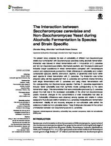
Like most surfaces, bridge decks and roads experience sensible, latent, radiative and ground heat fluxes (Figure 1a). For bridge decks, the bottom surface heat transfer from net radiation and sensible heat must also be considered. The energy balance for a concrete bridge deck in its active state also includes the internal hydration heat source from the concrete’s binding components (cement, microsilica, and flyash for Class HP concrete used by the New York State Department of Transportation (NYSDOT 1999), a variation of Class H concrete binder which contains cement and flyash). Excess water from irrigation hoses is sprayed on the curing deck’s top surface (covered with burlap) for several days to facilitate the top surface hydration reactions and to remove heat.

QGA Form

X Q*B

Form

Styrofoam

Burlap and Hoses f. f. f. f. f . 24 cm f. f. f. f. f.

QGB:

QGB

X

QHB Key: QRA: Q*A: QHA: QEA: QGA: Q*B: QHB:

Concrete

b. b. b. b. b. b. b . 30 cm b. b. b. b. b.

Support Beam

Top surface runoff water heat flux Top surface net radiative heat flux Top surface convective heat flux Top surface evaporative heat flux Top surface concrete heat flux Bottom surface net radiative heat flux Bottom surface conductive and convective heat flux Bottom surface concrete heat flux

b.

I

The hydration reactions consist of four stages, each distinct in their heat generation rates (Figure 1b). Upon mixing with water, surface reactions produce a ‘gel’ on cementitious particles and release heat (Stage I). The presence of the gel impedes the diffusion of water into the cement particle slowing the hydration for several hours (Stage II). When the water reaches the unhydrated cement, vigorous hydration and heat development occurs lasting up to 24 h (Stage III; setting occurs at the beginning of Stage III). After Stage III, the hydration reactions diminish considerably but will continue for many years (Stage IV). The deck is essentially a passive volume during Stage IV. Stage II can be extended by the addition of small amounts of retarders, generally in liquid form, into the concrete mix. The use of retarders is often necessary for large pours of concrete where the setting of one area before another could lead to cracking. By increasing the length of Stage II with retarders, this problem can be avoided. For more details of cement and concrete chemistry, see Neville (1996), Taylor (1997), Wojcik et al. (2001) and Wojcik (2001). The first estimates of the magnitudes of heat transfer mechanisms for curing bridges were determined by Wojcik and Fitzjarrald (2001) for four bridges in eastern and central New York in 1995, 1996, 1998 and 1999. They found that the magnitude of each transfer term varied according to the atmospheric conditions, suggesting that concrete conditions will vary depending on season, location and time of placement. Between 70 and 85% of the heat transfer occurred at the top surface and most was transferred by evaporation or the runoff water, with the evaporation dominating when wind speeds were >1 m s−1. The total amount of heat that was lost through the top surface at night during Stage III was up to three times greater (360 W m–2 compared with 120 W m−2) than that when the bridge was no longer generating significant heat (Stage IV), indicating the vigour of the hydration reactions. Steel beams supporting the concrete from below (Figure 1a)

166

J kg-1 s-1

III

IV

II

Time (h)

Figure 1. (a) Schematic cross-section of a bridge deck indicating the energy balance terms used as boundary conditions in the SLABS model. Not to scale. The concrete thickness averaged about 29 cm and the minimum width of the bridges studied was 9.8 m. The arrows indicate the typical direction of energy flow when the peak concrete temperatures occur during the night; ‘b’ and ‘f’ indicate grid points above a beam and the form, respectively. (b) A typical example of heat generation rates (J kg−1 s−1) for hydrating cement. Roman numerals indicate the stages in the hydration process.

also transferred significant heat, but this heat transfer was limited to the regions directly above the beams, or ~20% of the bottom surface area of the bridge decks.

1.2. Boundary condition validation in road model systems Some road models employ surface energy balance techniques to predict the road surface temperatures and road moisture type and amount (e.g. Rayer 1987; Sass 1997; Crevier & Delage 2001). Other road models also use statistical techniques with current and historical data (e.g. Shao & Lister 1996; Jacobs 1997). While predictions of road surface temperatures by the energy balance models are within 2 °C of the observed values at many times, their validation procedures and the model flux parameterisations have limitations. For example, these models use surface layer similarity hypotheses and assumed roughness lengths to compute exchange coefficients for convective fluxes in road environments. These road environments do not represent homogeneous conditions, as this type of similarity

Modelling the atmosphere/concrete interaction requires (e.g. Chen et al. 1999). Another limitation is that only the surface temperature predictions and not the surface flux predictions are verified. Radiation is the dominant term in the surface energy balance (e.g. Wojcik & Fitzjarrald 2001). Some radiation parameterisations in these models are highly detailed, including information about aerosols, ozone and shading effects (Rayer 1987; Sass 1997; Crevier & Delage 2001). However, no radiation measurements are made at typical roadside weather stations and we have found no comparisons of observed and predicted values of any of the road surface flux terms. Furthermore, systematic biases in temperature predictions are sometimes arbitrarily fixed by applying a correction factor to the radiation terms until the observed and predicted temperatures match (e.g. Crevier & Delage 2001).

1.3. Current concrete placement and curing specifications To attain its maximum service life and durability, concrete should develop low permeability and porosity to reduce the ingress of water, road chemicals and other pollution. Placement and curing specifications are implemented so that such properties develop by ensuring that: • •

•

the concrete temperatures and temperature gradients do not become too large, the concrete doesn’t freeze, which would limit hydration and produce cracking due to the expansion of freezing water, and the concrete top surface remains moist.

These factors, as well as temperature and stress development during the first several hours of hydration, the rigidity of the mass during the cooling phase of the hydration, and the degree of structural restraint, will determine the concrete quality (Emborg 1990; Roelfstra et al. 1994; Mangold & Springenschmid 1994). The stresses, restraints and rigidity of the concrete mass are beyond the scope of the present study and we focus on the concrete temperatures. While moist curing for a period of several days or more is widely used for bridge decks, there is no consensus

about other curing and placement conditions (Table 1). For example, NYSDOT states that the air temperature at the time of placement and during curing should not be below 7 °C (NYSDOT 1998), while the Minnesota Department of Transportation (MNDOT) declares that it should not be below 2 °C (MNDOT 2002). The MNDOT specifications also state that as long as moist curing is applied, normal air temperatures in spring, summer and fall are not detrimental to the concrete. The American Concrete Institute (ACI), however, reports that the concrete quality may suffer under high ambient air temperatures (ACI 1991). Because conditions and materials vary widely, the ACI asserts that it is impractical to recommend a limiting air or concrete temperature above which the quality of the concrete will be greatly diminished. Finally, the ACI suggests that the evaporation rate during the placement should not exceed 680 W m−2 (ACI 1991), while the NYSDOT states that it should not be above 830 W m−2 (NYSDOT 1998). We note that, in practice, ensuring good curing can be very difficult on site due to construction schedules, environment issues and construction features. A field engineer who must follow such specifications, among other duties, is responsible for determining the best time for the concrete to be placed, the best curing procedures, and the best mix design so that the concrete can attain its best possible strength and durability while keeping construction costs within budgetary limits. The NYSDOT and MNDOT specifications are based on studies that had unrealistic boundary conditions and so may be of little use to engineers. Furthermore, because the interaction between the heat and water transfer and the hydration reactions determines the thermal and moisture states of the curing concrete, the concrete conditions will vary depending on the season and location. Therefore, the application of such specifications to all freshly placed concrete is dubious, emphasising the need for an operational field forecast model to determine the best time to pour, the best mix design, or the best curing practices based on predicted concrete conditions. We have developed the SLABS model to study the sensitivity of concrete temperatures and moisture to atmospheric and construction conditions and to comment on the practicality of current placement and

Table 1. Current concrete placement and curing specifications for several agencies. Specification

NYSDOT

MNDOT

ACI

Initial Concrete Temperature Evaporation Rate at Placement Air Temperature at Placement and during Curing

— ≤830 W m–2 ≥7 °C

10–32 °C — ≥2 °C

— ≤680 W m–2 ≤24–38 °C

Moist Curing with burlap for 14 days (burlap placed within 30 minutes of concrete placement) —

Moist Curing with burlap

Moist Curing with burlap

—

3 oC h–1 or 28 oC day–1

Curing Method

Concrete Cooling Rate

167

G S Wojcik, D R Fitzjarrald & J L Plawsky curing specifications. In the process, we have validated our model boundary conditions with both estimated and measured bridge temperatures and fluxes, addressing a limitation of previous road modelling studies. The model is simple enough to allow a field engineer to make appropriate on-site decisions based on weather forecasts, and is flexible enough to accurately account for the heat and mass transfer that occurs in any atmospheric conditions. In the following, we provide a description of the SLABS model in section 2, which also includes a discussion of the boundary conditions and the heat generation formulation. In section 3, we evaluate the model boundary condition parameterisations and the model’s sensitivities to various physical and chemistry parameters. We also present in section 3 an analysis of the sensitivity of the model predictions of concrete temperatures, binder concentrations and water concentrations to: (i) many atmospheric conditions including those in various climates and seasons; and (ii) construction practices such as the time of placement and the initial concrete temperature. In section 3, we also comment on current curing and placement specifications and apply the model as an operational forecast model to one of the bridges studied in our field work. This work is summarised in section 4.

2. Methodology In a typical bridge that we studied (Wojcik & Fitzjarrald 2001), the concrete had different thicknesses depending on the given horizontal location (Figure 1a). The concrete is ~6 cm thicker over the steel support ‘I’ beams (30 cm) than it is over the ‘form’ (a thin, shiny, corrugated, galvanised steel sheet supporting the concrete from below) (24 cm). The steel beams and half of the steel form are in direct contact with the concrete. The other half of the steel form is covered by styrofoam to reduce the amount of concrete that is used. At the top surface, the concrete was covered with burlap and sprayed with water from irrigation hoses for up to 14 days after placement.

2.1. SLABS model The SLABS model is a 1D finite difference model which solves the governing equations by using a fully implicit Crank-Nicolson scheme for the diffusion of heat and moisture (Press et al. 1992: 637−640) and a fourth-order Runge-Kutta scheme for the chemistry (Press et al. 1992: 550−554). For simulations of locations at or above the form, the SLABS model consists of ten vertical grid points (nine layers) with a grid size of 2.7 cm and predicts the vertical temperatures and water and binder concentrations in the concrete slab (Figure 1a). When applied over the beams, the model

168

consists of 12 vertical grid points (11 layers). Each grid point corresponds to a point at which the NYSDOT took vertical concrete temperature measurements. The governing equations are: Binder concentration, B (molB mcon−3 (con=concrete)): dB = − k ⋅ B n ⋅ Rm dt

(1)

where R (molR mcon−3) is the concentration of water available for the hydration reactions; n and m are exponents whose sum gives the order of the hydration reaction (n=m=1); k (mcon3 molR−1 s−1) is the reaction rate constant given by: Ea (2) ) R* ⋅ Tc where Ea is the activation energy, A is the preexponential factor; R* is the universal gas constant (8.314 J mol−1 K−1), and Tc (K) is the concrete temperature. Wojcik et al. (2001) provided justification for n=m=1, determined that Ea=35 kJ mol−1 and found A=0.0015−0.0033 for simple calorimetry experiments. k = A ⋅ exp(−

Concrete temperature, Tc: ∂ 2Tc dTc dB = KT −V ⋅ 2 dt dt ∂z

(3)

where the second term on the right hand side of Eq. (3) is the hydration heat source term where V (K mcon3 molB−1 s) converts the reacted binder concentration to heat and is equal to −∆H*MwB/ρccpc; −∆H: the hydration heat of Class HP concrete (~ 420 kJ kgbinder−1); cpc: the specific heat of Class HP concrete (~ 1380 J kg−1 K−1); and ρc: the density of Class HP concrete (~2230 kg mcon−3). KT is the thermal diffusivity of concrete (~8.8x10−7 mcon2 s−1), determined from ρc, cpc, and the Class HP thermal conductivity, kc (~2.7 W m−1 K−1). − ∆H was determined with calorimetry experiments and ρc and cpc were calculated from a concrete sample taken from the batch used at the 1999 bridge (Wojcik & Fitzjarrald 2001; Wojcik et al. 2001). Wojcik & Fitzjarrald (2001) determined kc from a heat flux plate and thermocouples placed within the concrete and with the SLABS model. MwB is the molecular weight of the binder (0.191 kg mol−1) determined from a mass average weighting of the molecular weights of cement (0.232 kg mol−1), flyash (0.077 kg mol−1), and microsilica (0.062 kg mol−1) (Watt & Thorne 1965; Hjorth 1982; Bureau of Reclamation 1988). Available water concentration, R (molR m−3): ∂2 R dR dB = KR 2 + η ⋅ dt dt ∂z

(4)

where KR (~10−9 m2 s−1) is the diffusivity of water in concrete (Pommershiem & Clifton 1991). R is the water concentration in the concrete that is available for the hydration reactions. We reduce KR by a factor of 20 (Powers 1958) when the binder hydration fraction

Modelling the atmosphere/concrete interaction reaches 0.6. At this hydration fraction, the larger pores in the concrete become segmented (Bentz & Garboczi 1991), significantly limiting the movement of water. The term η in Eq. (4) represents the number of moles of water removed from the available pool per mole of binder that hydrates. Some water is chemically converted into the hydration products and some is adsorbed onto the surface of the hydration products where it cannot be used for further hydration (Powers & Brownyard 1946−7). Both sinks are taken into account in η. To determine η and A in Eq. (3), we minimised the temperature root mean square error, RMSE, for the 1999 bridge by varying η and A over wide ranges. We determined A=0.0039 and η=8.3. See also section 3.3 for more details on this procedure. At both the top and bottom surfaces of the bridge deck, the boundary conditions are implemented in fluxconservative form (e.g. Press et al. 1992: 825−838). Such a format is chosen to maintain the stability of the solutions by keeping the second-order accuracy of the implicit Crank-Nicolson scheme. By convention, upward fluxes are positive. For the top surface, the energy balance (W m-2) is given by: -Q*A + QGA = QHA + QEA+ QRA

(5)

where Q*A is the net radiation; QGA is the heat flux through the concrete top surface; QHA is the sensible heat flux; QEA is the heat flux due to the evaporation of water; and QRA is the runoff water heat flux (Figure 1a). The top surface energy flux (QGA) is given by: QGA = − kc

dTc = dz

−QA* − ρLvCeU (qa − qs ) − ρc pChU (Ta − Ts ) − ρwc w (Twi − Twf )

(6) M Atop

The second term on the right hand side of Eq. (6) is the latent heat flux, the third is the sensible heat flux, and the fourth is the runoff water heat flux. M represents the volume flow rate of water running off the bridge (m3 s−1); Atop is the area of the bridge’s top surface (m2); qa and qs are the air and surface specific humidities (g g−1); Ta and Ts are the air and surface temperatures (°C); ρw and ρ are the water and air densities (kg m−3); cw and cp are the water and air specific heat capacities (J kg−1 K−1); Lv is the latent heat of evaporation (J kg−1); U is wind speed (m s−1); Ce and Ch are dimensionless exchange coefficients; z is the vertical dimension (m); and Twi and Twf are the initial (when hitting the top surface) and final (when running off the bridge) spray water temperatures (°C)

The exchange coefficients, Ce=Ch, for conditions other than free convection (free convection assumed when the bulk Richardson number, Rb, < −1 and U < 1 m s−1) were determined by Wojcik & Fitzjarrald (2001) from field measurements and subsequent development of the energy balances of the four curing concrete bridges. Free convection exchange speeds (equal to CU in Eq. 6) are given by the parameterisation of Kondo & Ishida (1997) for a smooth surface. The net radiation, the dominant term in the top surface energy balance (Wojcik & Fitzjarrald 2001), is computed in the model by determining the incoming and outgoing longwave and shortwave radiation components. The clear sky, incoming shortwave radiation at the surface (KI) was calculated with a scheme given by Stull (1988: 257−258). The effect of cloud cover fraction, clf, on KI is given by Freedman et al. (2001) as: K I = 0.91 − (0.7 ⋅ clf )

(7)

The outgoing shortwave radiation, KO, is equal to 0.14*KI, where 0.14 is the albedo of concrete covered with burlap and sprayed with water (Wojcik & Fitzjarrald 2001). The clear sky incoming longwave radiation (LI) is given by Stefan-Boltzman’s law. The atmospheric emissivity for clear skies, εclear, as a function of atmospheric water vapour pressure (ea) and air temperature (Ta), is determined with a scheme proposed by Prata (1996):

ε clear

1   ea  ea  2    = 1 −  1 + 46.5 ⋅  ⋅ exp− 1.2 + 3 ⋅ 46.5 ⋅  (8) Ta  Ta       

For cloudy skies, the atmospheric emissivity, as a function of vapour pressure, temperature, and clf is given by Brutsaert (1975): 1

ε cloudy

e 7 = clf + 1.24 ⋅ (1 − clf ) ⋅  a   Ta 

(9)

The outgoing longwave radiation (LO) is given by Stefan-Boltzman’s law with a surface emissivity of 0.98 for the wet surfaces of the bridges. Wojcik & Fitzjarrald (2001) determined that these parameterisations generally predict Q*A within ±60 W m−2, although the predictions may be as much as 100 W m−2 (15%) too high during the mid-afternoon on sunny days. The temperature of spray water as it hits the top surface (Twi) is determined by assuming the drop temperatures adjust to the environmental conditions as they rise and fall after being ejected from irrigation hoses (Wojcik & Fitzjarrald 2001), as given by a model by Pruppacher & Klett (1997). The drops generally do not remain airborne long enough to approach the air wet-bulb temperature. By assuming they do can result in errors in

169

G S Wojcik, D R Fitzjarrald & J L Plawsky QRA of more than 25% (Wojcik & Fitzjarrald 2001). The runoff water temperature (Twf) was assumed to be the top surface concrete temperature, as suggested by Wojcik & Fitzjarrald (2001). When the effects of spray water are simulated, we assume that there is a puddle of water on the top surface (R=55555 molR mR−3) for the top surface water boundary condition. At the form, the heat flux at the bridge bottom, QGB (W m−2), is given by: QGB = − kc

dTc = QB* + ρc pUCb (Ta − Tcf ) dz

(10)

where the second term on the right-hand side accounts for convective heat loss; Tcf is the temperature of the form; Q*B is the net radiation at the bottom surface; and Cb is the exchange coefficient for the form. The layer of air between the beams had a stable stratification (warmest air near the form) and so convective heat loss from the form was small (Wojcik & Fitzjarrald 2001). As such, Cb is set to 10−5 in the model. Q*B at the form was computed by applying Stefan-Boltzman’s law to the surface below the bridge and the form for the upward and downward longwave fluxes with the form emissivity of 0.1 and the ground emissivity of 0.98 (water/soil). The net radiation at the form is generally 25 W m−2 < Q*B< 25 W m−2 much of the time (Wojcik & Fitzjarrald 2001). Heat transfer through the top of the steel support beams (Figure 1a) is modelled as heat flow through an infinite steel fin (Incropera & DeWitt, 1996, pp. 118). The beam heat loss ( = QGB when considering just the beam), Fbeam (W m-2), is given by:

1

Fbeam = −

(Tcs − Ta ) ⋅ (hPks Acf ) 2

(11)

Atb

where h is the heat transfer coefficient for free convection from a vertical flat plate (Incropera and DeWitt 1996: 457); P is the perimeter of the fin; Acf is the crosssectional area of the fin; Atb is the surface area of the beam in contact with the concrete; Tcs is the temperature at the concrete-steel interface and ks is the thermal conductivity of the steel beam (~ 65 W m−1 K−1). This localised heat transfer can be up to 150 W m−2 during the active stage of the hydration reactions, or ~50% of that at the top surface during this time (Wojcik & Fitzjarrald 2001), resulting in horizontal temperature gradients near the bottom of the deck as large as the vertical gradients at the top surface (see section 3.6).

2.2. Boundary condition sensitivity simulations We examined the model’s temperature, moisture, binder and heat predictions for two different categories of atmospheric boundary conditions: (i) diurnal boundary conditions (DBC) and (ii) seasonal/climate boundary conditions (SBC). The variables considered were air temperature and humidity (Ta and RH), wind speed (U) and cloud cover fraction (clf). The range of values chosen represents typical conditions observed in the atmosphere (Table 2). In preliminary simulations with variations of one variable at a time, the concrete temperatures were most sensitive to Ta, RH, and U,

Table 2. Results of the diurnal boundary condition (DBC) model simulations for atmospheric variables when just one variable was varied at a time. The “Baseline” row gives the baseline value for each variable. The “Baseline Range” row shows the range used for each boundary value. The ranges given in the “Baseline Range” row are afternoon values except for clf. In the “Peak”, “Stage III”, and “Stage IV” rows are given the equations which predict these temperatures as a function of the boundary variable. The R2 value is given in parentheses underneath each equation except for U which displays the residual standard error of a polynomial fit. The temperatures in parentheses beside the titles “Peak”, “Stage III”, and “Stage IV” are the values for the Baseline simulation. Note that the Stage III and Stage IV temperatures are averages over the first 24 h of each stage. The “Range” rows indicate the range of predicted temperatures over the range of the given boundary variable for the temperature category given in the row above each.

Baseline Baseline Range Peak (43.7 °C) Range Stage III (30.6 °C) Range Stage IV (22.6 °C) Range a

Ta ( °C)

RH (%)

U (m s-1)

clf

25 0-45a

70 0-100b

3 0.5-10c

0 0-1

33.5+0.48*Ta (0.99) 35.9-52.7

36.9+0.09*RH (0.95) 36.9-45.9

51.5-5.7*U +0.57*U2 (0.43) 50.5-38

42.8-4.77*clf (0.99) 42.8-38.0

21.20+0.47*Ta (0.99) 23.5-40.0

25.0+ 0.08*RH (0.99) 25.0-33.0

36.0-3.2*U +0.37*U2 (0.25) 35.5-27.5

30.2-2.5*clf (0.99) 30.2-27.7

10.9+0.62*Ta (0.99) 14.0-35.7

16.1+0.10*RH (0.99) 16.1-26.1

28.3-3.7*U +0.39*U2 (0.39) 27.9-20.3

22.7-2.6*clf (0.99) 22.7-20.1

Afternoon–morning temperature pairs (oC): 45–35, 40–30, 35–25, 30–20, 25–15, 20–10, 15–5, 10–0. relative humidity pairs (%): 0-0, 0–60, 10–70, 20–80, 30–90, 40–100, 100–100. c Afternoon–morning wind speed pairs (m s-1):10–0.5, 8–0.5, 6–0.5, 4–0.5, 2–0.5, 0.5–0.5. b Afternoon–morning

170

Modelling the atmosphere/concrete interaction with peak temperatures changing by 9 °C or more over the ranges tested. Note that temperatures were nonlinearly related only to U and most sensitive to U when U < 2 m s−1 (Table 2).

a. Ta (oC)

Local Time

For the DBC simulations, typical diurnal variations of Ta, RH and U are emulated with the following equations: St = S + N S ⋅ cos(t ⋅

2π ) 24

SPM − SAM 2

RH (%)

(12)

where S¯t is the value of either Ta, RH or U at time t (h); S is the daily average value of variable S; NS is the amplitude of the diurnal wave of the given variable: NS =

b.

Local Time c. U (m s-1)

Local Time

(13)

where the subscripts PM and AM indicate the extreme values of S at 1600 and 0400 local time (LT), respectively (Figure 2). While producing smoother temporal variations of these variables than are actually encountered in the atmosphere, this formulation captures the main features of typical diurnal variations. Ta and U generally peak during the late afternoon while RH reaches a minimum during this time. Note that with this formulation, qa in Eq. (6), is determined both as a function of RH and Ta. The DBC simulations were run for Albany, New York in early June with the concrete being placed at 0700 local time. The length of Stage II was set at eight hours. The variations of incoming solar radiation with time of day and time of year were computed with schemes discussed in section 2.1. With the DBC, we also studied how construction practices might influence the concrete heat generation and temperatures. For these cases, we varied the volume of water sprayed onto the deck (W), the initial tempera-

Figure 2. (a) Example of diurnal air temperature variations used for the diurnal boundary condition (DBC) simulations. (b) as in (a), but for relative humidity. (c) as in (a), but for wind speed.

ture of that water as it left the hoses (Td0), the concrete temperature at the time of placement (Tc0) (Table 3), and the time of placement. These factors potentially can be controlled at the discretion of construction personnel or the field engineer. For the bridges we studied in the field, W ranged from 2.4 mm hr−1 to 15 mm hr−1. Tc0 for the bridges ranged from 23 °C to 29 °C and Td0 from 15 ºC to 29 ºC (initial spray water temperature data are available only for the 1998 and 1999 bridges). We expanded the ranges of these variables for the construction practice simulations to broaden the scope of our investigation. In preliminary simulations with variations of one construction variable at a time, the concrete temperatures were most sensitive to Tc0 with peak temperatures increasing by more than 15 ºC over the range tested (Table 3).

Table 3. Results of the diurnal boundary condition (DBC) model simulations for construction practice variables. The “Baseline” row gives the baseline value for each variable. The “Baseline Range” row shows the range used for each boundary value. In the “Peak”, “Stage III”, and “Stage IV” rows are given the equations which predict these temperatures as a function of the boundary variable, with the R2 value in parentheses underneath each equation. The temperatures in parentheses beside the titles, “Peak”, “Stage III”, and “Stage IV” are the values for the Baseline simulation. Note that the Stage III and Stage IV temperatures are averages over the first 24 h of each stage. The “Range” rows indicate the range of predicted temperatures over the range of the given boundary variable for the temperature category given in the row above each.

Baseline Baseline Range Peak (43.7 °C) Range Stage III (30.6 °C) Range Stage IV (22.6 °C) Range

W (mm h-1)

Tc0 ( °C)

Td0 ( °C)

14 0–52

25 5–40

25 5-40

43.7–0.062*W (0.98) 43.7–40.5

32.7+0.45*Tc0 (0.99) 35.0–50.7

40.2+0.1*Td0 (0.99) 40.7–44.2

31.2–0.054*W (0.97) 31.2–28.4

25.4+0.21*Tc0 (0.99) 26.5–33.8

27.1+0.12*Td0 (0.99) 27.7–31.9

22.8–0.011*W (0.97) 22.8–22.2

22.7–0.001*Tc0 (0.86) 22.7

18.7+0.16*Td0 (0.99) 19.5–25.1

171

G S Wojcik, D R Fitzjarrald & J L Plawsky To examine how the predicted concrete heat generation and temperatures would vary depending on the season and geographical location (SBC simulations), we used average climate data from the Northeast Regional Climate Center at Cornell University, Ithaca, NY, for Albany, New York (temperate climate), Tampa Bay, Florida (tropical), Phoenix, Arizona (desert), and Fairbanks, Alaska (cold) for the atmospheric boundary conditions. These data consist of the daily average maximum and minimum temperatures and relative humidities, and daily average wind speeds for January, April, July and October (Table 4). The time of placement was 0700 local time and the length of Stage II was set to 8 h. For all simulations, we compared the mean concrete temperatures over the first 24 h of Stage III and Stage IV and the peak Stage III concrete temperature. In addition, we compared the peak temperature gradients in Stages III and IV and the 24 h and 72 h cumulative heat generation and hydration fractions.

3. Results 3.1. Validation of SLABS model boundary conditions To validate the model boundary conditions, we determined the predicted concrete temperature RMSE with predicted temperatures and those measured by NYSDOT for all grids when the concrete was no longer

generating significant heat (after about 40 h after the pour) and local fluxes of heat and moisture determined the concrete’s thermal structure (Stage IV). We performed simulations with the observed 1998 and 1999 conditions which, respectively, featured cloudy, cool, moist atmospheric conditions and sunny, warm, dry atmospheric conditions. We compared model predictions of the surface fluxes to the energy balance estimates for these bridges from the field work. Because up to 85% of the heat transfer above the form occurred through the top surface (Wojcik & Fitzjarrald 2001), we focused mainly on the top surface fluxes. We also evaluated the predicted heat transfer through the steel support beams where heat transfer of up to 150 W m−2 was observed. For simulations of concrete temperatures over the form, the model produced RMSE of ~1 ºC during the day and night for both bridges. Figure 3 shows predicted and observed concrete temperatures for the 1999 bridge. During the daytime, QGA was underpredicted by about 10−30%, and during the night QGA was overpredicted by < 30%. The underprediction during the daytime was the result of overpredictions of −Q*A (~15% at peak) that enhanced QEA, QHA and QRA. During Stage IV above the beams, the predicted RMSE was about 1.7 ºC for both bridges (e.g. Figure 3). Note that the predicted temperatures over the beam during Stage III were up to 5 ºC lower than those over the form, as seen in the observations. For the 1999

Table 4. Climate information for the four cities used in the SBC model simulations. The data were obtained from the Northeast Regional Climate Center at Cornell University in Ithaca, NY USA. Temperature data are for years 1961-1990 and humidity and wind data are for at least 45 years up to 1998.

July RH Afternoon (%) RH Morning (%) Ta Afternoon (°C) Ta Morning (°C) U Mean Daily (m s-1) October RH Afternoon (%) RH Morning (%) Ta Afternoon (°C) Ta Morning (°C) U Mean Daily (m s-1) January RH Afternoon (%) RH Morning (%) Ta Afternoon (°C) Ta Morning (°C) U Mean Daily (m s-1) April RH Afternoon (%) RH Morning (%) Ta Afternoon (°C) Ta Morning (°C) U Mean Daily (m s-1)

172

Phoenix, AZ

Tampa, FL

Albany, NY

Fairbanks, AK

20 43 41 27 3.2

63 87 32 23.6 3.2

55 81 29 15 3.4

50 69 22 11.4 2.9

22 49 31 16 2.6

58 89 29 18.4 3.8

58 86 16.6 4.6 3.6

67 79 0 -6.9 2.4

32 65 18.8 5 2.4

60 87 21 10 3.2

63 78 -1 -11.7 4.4

70 69 -18.7 -28 1.3

16 42 29.2 12.9 3.1

52 87 27.6 16 4.1

49 72 14.2 1.7 4.7

45 60 5 -6.4 2.9

Modelling the atmosphere/concrete interaction b.

a.

Z (cm)

Z (cm)

T (oC)

T (oC)

temperatures for this analysis, as we did with the boundary condition validation. For these comparisons, Ea=35000 J mol−1, A=0.0039 and η=8.3 (see section 3.3). By varying kc from 2 to 4 W m−1 K−1, the largest change in RMSE from the baseline value was 0.8 ºC. Variations of KR from 10−8 to 10−12 m2 s−1, ρc from 2100 to 2400 kg m−3, and cpc from 1300 to 1460 J kg−1 K−1 changed the RMSE by at most 0.3 ºC. The largest change in RMSE from the baseline value when −∆H was varied from 360 to 540 kJ kg−1 was 1.8 ºC.

d.

c.

3.3. Determining and validating η and A Z (cm)

Z (cm)

T (oC)

T (oC)

Figure 3. Observed and predicted vertical profiles of concrete temperatures above the beam, ‘1’ and ‘2’, respectively, and observed and predicted vertical profiles of concrete temperatures above the form, ‘3’ and ‘4’, respectively. Distances, Z, are distances above the top of the beams. ‘Sfc’ indicates the top surface. (a) At 2300 LT on 10 June 1999, the approximate time of peak concrete temperatures (Stage III); (b) as in (a), but for 1300 LT on 11 June (Stage III); (c) as in (a), but for 1300 LT on 13 June (Stage IV); (d) as in (a), but for 0200 LT on 14 June (Stage IV).

bridge, predicted heat transfer through the beams was 25 W m−2 during the daytime and −100 W m−2 during the night, while the values estimated from the field measurements were about 20 W m−2 during the daytime and −80 W m−2 during the night. Because the model top surface and beam fluxes were within 30% of those determined from the field observations during most times for both bridges, and because the predicted temperatures were within 2°C of the observed values during the day and night, we feel our boundary condition parameterizations (in conjuction with the values for ρc, cpc, and kc; see section 3.2) are reasonable.

3.2. Sensitivity of predicted temperatures to model parameters SLABS uses a set of parameters whose values are uncertain to varying degrees. The uncertainties for kc, ρc and cpc are, respectively, ±30%, ±1% and ±10% (Wojcik & Fitzjarrald 2001) and for −∆H is ±15% (Wojcik et al. 2001). We tested the model sensitivity to these parameters and KR by comparing the RMSE from a simulation with a baseline set of parameter values given in section 2.1 with the RMSE from simulations with perturbation parameter values determined from the uncertainty estimates. We focused only on Stage IV

To determine A and η, we optimised the model’s RMSE over the first 36 h of Stage III for the 1999 bridge by varying A and η, respectively, over the ranges of 0.002 2 m s−1. Peak concrete temperature gradients were found near the top surface and the steel support beam tops around the time of peak concrete temperatures and ranged from −2 ºC cm−1 to 1 ºC cm−1. The rule-of-thumb critical top to bottom concrete tem-

6.

7.

8.

perature difference of 20 ºC, above which the concrete may crack, may be exceeded when the initial concrete temperature is greater than 20 ºC and the afternoon air temperature is less than 35 ºC. To achieve the lowest concrete temperatures and temperature gradients, the time of the pour should be during the late afternoon or evening (based on an eight-hour set delay due to retarders) and the initial concrete temperature should be kept at or below 25 ºC, especially when wind speeds are < 2 m s−1. Morning pours result in the highest concrete temperatures and temperature gradient magnitudes. Concrete temperatures in July at Tampa and Phoenix (which on average has higher air temperatures and lower humidities than Tampa in July) were found to be similar. The effect of the higher air temperatures on concrete temperatures at Phoenix was offset by greater evaporation rates. Such compensation reiterates the need to include all important boundary forcings in models of curing concrete. Generally, evaporation rates increased for decreasing air temperatures and humidities and increasing wind speeds and surface concrete temperatures. For wind speeds < 2 m s−1, the evaporation rate will likely remain < 830 W m−2 (the NYSDOT critical

183

G S Wojcik, D R Fitzjarrald & J L Plawsky

9.

rate) for all surface concrete temperatures and air temperatures and humidities. When heat is removed from the concrete by evaporation, the evaporation rate increased by a factor of 2−2.5 for an increase in surface concrete temperatures of 10 ºC. Evaporation rates determined from a nomogram were about 15−35% lower than those from our evaporation parameterisation. The SLABS forecast model, which uses numerical weather prediction model forecasts as input, outputs peak temperature and temperature gradient predictions, placement- time evaporation rates, and warning messages about conditions hazardous to the concrete. Temperature predictions from the forecast model were shown to be within 2 ºC of observed temperatures at the 1999 bridge showing the model’s utility as an operational field model. This application of the model showed that local effects on atmospheric conditions will influence the concrete temperatures. Specifically, obstacles acting as wind breaks can be accounted for with schemes such as that suggested by Acevedo (2001).

4.2. Discussion The analysis presented here shows clearly that atmospheric and construction conditions can have a significant effect on curing concrete temperatures. Note that the results are specific for NYSDOT’s Class HP concrete; other concretes may have different sensitivities. The wide range of atmospheric and construction conditions that may be encountered and the lack of data relating temperature effects to stresses in Class HP concrete make it difficult to devise a detailed set of placement and curing specifications based on the results presented here. Until more information on stress development is available, the SLABS forecast model can be used by field engineers as a guide to determine the best time for placement or the best mix design or curing practices to implement. The SLABS forecast model has been shown to be an efficient and accurate tool with which to predict concrete temperatures based on the data we collected at four bridge decks. While our observational datasets are the most extensive ever taken for bridge decks to our knowledge, the model can only be improved and its performance further evaluated with the collection of more observational data. To make the model more useful, information about the effect of various doses of retarders on hydration rates and set delay must be determined. Experience of the field engineer or concrete plant personnel aids the determination of the dosage rate to give a certain set delay. However, the lack of information on retarder/hydration effects casts some uncertainty on

184

the ability of the forecast model to provide accurate temperature predictions. Our analysis suggests that late afternoon or early evening is generally the best time to pour concrete, based on the criteria of keeping the concrete temperatures and temperature gradients as low as possible. However, the concrete plants, construction companies and their employees may not be willing to adjust their normal operating schedules to facilitate late afternoon pours. Pouring late in the day may require the use of artificial lighting, another expense for the companies. There is also the risk that if some part of the placement and finishing operation goes wrong, the necessary part or personnel may not be available to resolve the problem, perhaps ruining the placement. Higher binder hydration fractions near the bridge top surface, due to its proximity to the spray water source, imply that there is a vertical gradient in strength. Such a gradient may be important to the concrete’s longterm durability as certain concrete sections may be affected differently by, for example, freeze-thaw cycles, the result being increased stresses within the concrete. Lower hydration fractions near the bottom of the deck could be mitigated by the addition of water-saturated lightweight aggregate to the concrete mix, perhaps reducing early thermal cracking (D. Bentz 2001, personal communication). More research on this topic is needed. The SLABS forecast model can be adapted to predict road temperatures and conditions. We have validated the SLABS model boundary conditions with field measurements and flux estimates. Surface flux predictions of existing road models have not been evaluated. One reason for the lack of validation of the radiation flux, the dominant term of the energy balance, is that radiation measurements are rarely, if ever, taken at road weather stations. Such measurements should be made not only for the validation procedure, but also to identify microclimates. With weather model forecasts and information from the planned 400 roadside weather stations in New York State, the SLABS model adapted to the road environment can be used by NYSDOT road maintenance personnel to determine when and where to use de-icing chemicals and how much to apply, perhaps saving millions of dollars each year by reducing the amount of chemicals used and by reducing the number of personnel hours. The reduction in chemicals will decrease the damage to ecosystems along roads and better road conditions will save lives.

Acknowledgements We gratefully acknowledge the partial funding support from the New York State Department of Transportation’s Research and Development Bureau and the Atmospheric Sciences Research Center at the

Modelling the atmosphere/concrete interaction University at Albany, State University of New York. We thank Dale Bentz of the Building and Fire Research Laboratory at the National Institute of Standards and Technology in Gaithersburg, Maryland for many valuable discussions and suggestions about the cement and concrete science portion of this work. We also thank two anonymous reviewers for their comments and suggestions which have improved this paper.

References Acevedo, O. (2001) Effects of temporal and spatial transitions on surface atmosphere exchanges. Ph.D. dissertation, University at Albany, State University of New York, 204 pp. ACI (1991) Hot weather concreting. ACI Materials Journal 4: 417−436. Bentz, D. P. (2002) Influence of curing conditions on water loss and hydration in cement pastes with and without flyash substitution. NISTIR 6886, 15 pp. [Available from the National Institute of Standards and Technology, 100 Bureau Drive Stop 8615, Gaithersburg, MD, 20899.] Bentz, D. P. & Garboczi, E. J. (1991) Percolation of phases in a three-dimensional cement paste microstructure model. Cem. Concr. Res. 21: 325−344. Bentz, D. P. & Hansen, K. K. (2000) Preliminary observations of water movement in cement pastes during curing using X-ray absorption. Cem. Concr. Res. 30: 1157−1168. Bogue, R. H. (1955) Chemistry of Portland Cement. Reinhold, 793 pp. Brutsaert, W. (1975) On a derivable formula for longwave radiation from clear skies. Water Resour. Res. 11: 742−744. Bureau of Reclamation (1988) Concrete Manual. US Department of the Interior, 627 pp. Chen, D., Gustavsson, T. & Bogren, J. (1999) The applicability of similarity theory to a road surface. Meteorol. Appl. 6: 81−88. Crevier, L.-P. & Delage, Y. (2001) METRo: a new model for road-condition forecasting in Canada. J. Appl. Meteorol. 40: 2026−2037. Emborg, M. (1990) Thermal stresses in concrete structures at early ages. Ph.D. dissertation, Luleå University of Technology, 286 pp. FitzGibbon, M. E. (1976a) Large pours for reinforced concrete structures. Concrete 10 (3): 41. FitzGibbon, M. E. (1976b) Large pours: 2. Heat generation and control. Concrete, 10 (12): 33−35. Freedman, J. M., Fitzjarrald, D. R., Moore, K. E. & Sakai, R. K. (2001) Boundary layer clouds and vegetation-atmosphere feedbacks. J. Climate 14: 180−197. Fujita, T. T. & Wakimoto, R. M. (1982) Effects of miso- and mesoscale obstructions on PAM winds obtained during project NIMROD. J. Appl. Meteorol. 21: 840−858. Gopalan, M. K. & Haque, M. N. (1987) Effect of curing regime on the properties of fly-ash concrete. ACI Materials Journal 84 (1): 14−19. Hjorth, L. (1982) Microsilica in concrete. Nordic Concrete Res. No. 1 Paper 9, Aalborg Portland, Denmark, 18 pp. Incropera, F. P. & DeWitt, D. P. (1996) Introduction to Heat Transfer, John Wiley & Sons, 801 pp. Jacks, E., Bower, J. B., Dagostaro, V. J., Dallavalle, J. P., Erickson, M. C. & Su, J. C. (1990) New NGM-based MOS guidance for maximum/minimum temperature, probability

of precipitation, cloud amount, and surface wind. Wea. Forecasting 5: 128−138. Jacobs, A. (1997) KALCORR: a Kalman-correction model for real-time road surface temperature forecasting. KNMI Report TR-198, 23 pp. [available from Applications and Modeling Division, KNMI, Netherlands.] Kondo, J. & Ishida, S. (1997) Sensible heat flux from the Earth’s surface under natural convection conditions. J. Atmos. Sci. 54: 498−509. Mangold, M. & Springenschmid, R. (1994) Why are temperature-related criteria so unreliable for predicting thermal cracking at early ages? In: R. Springenschmid, ed., Thermal Cracking in Concrete at Early Ages, Rilem Proceedings Series, Spon Press, 361−368. MNDOT (cited 2002) [available online at: www.mrr.dot.state.mn.us/pavement/concrete/ concrete.asp.] Neville, A. M. (1996) Properties of Concrete. Wiley & Sons, 844 pp. NYSDOT (1998) Bridge deck construction specification improvements-implementation of recommendations by the Bridge Deck Task Force. NYSDOT Rep. EI 98-037, 13 pp. [available from New York State Department of Transportation Structures Division, 1220 Washington Ave., Building 5, 6th floor, W. Averell Harriman State Office Building Campus, Albany, NY, 12232-0600.] NYSDOT (1999) Specification revisions − Class HP concrete for substructures and structural slabs. NYSDOT Rep. EI 99-002, 22 pp. [available from New York State Department of Transportation Structures Division, 1220 Washington Ave., Building 5, 6th floor, W. Averell Harriman State Office Building Campus, Albany, NY, 12232-0600.] Papadakis, V. G., Fardis, M. N. & Vayenas, C. G. (1992) Hydration and carbonation of pozzolanic cements. ACI Materials Journal 89 (2): 119−130. Pommersheim, J. M. & Clifton, J. R. (1991) Models of transport processes in concrete. NISTIR 4405, 92 pp. [available from the National Institute of Standards and Technology, 100 Bureau Drive Stop 8615, Gaithersburg, MD 20899.] Powers, T. C. (1958) Structure and physical properties of hardened Portland cement paste. J. Amer. Ceramic Soc. 41: 1−6. Powers, T.C. & Brownyard, T. L. (1946−7) Studies of physical properties of hardened Portland cement paste (nine parts), J. Amer. Concr. Inst. 43. Prata, A. J. (1996) A new long-wave formula for estimating downward clear-sky radiation at the surface. Q. J. R. Meteorol. Soc. 122: 1127−1151. Press, W. H., Teukolsky, S. A., Vetterling, W. T. & Flannery, B. P. (1992) Numerical Recipes in FORTRAN: The Art of Scientific Computing. Cambridge University Press, 966 pp. Pruppacher, H. R. & Klett, J. D. (1997) Microphysics of Clouds and Precipitation. Kluwer Academic Publishers, 954 pp. Rayer, P. J. (1987) The Meteorological Office forecast road surface temperature model. Meteorol. Mag. 116: 180−191. Roelfstra, P. E., Salet, T. A. M. & Kuiks, J. E. (1994) Defining and application of stress-analysis- based temperature difference limits to prevent early-age cracking in concrete structures. In: R. Springenschmid, ed., Thermal Cracking in Concrete at Early Ages, Rilem Proceedings Series, Spon Press, 273−280. Sass, B. H. (1997) A numerical forecasting system for prediction of slippery roads. J. Appl. Meteorol. 36: 801−817. Shao, J. & Lister, P. J. (1996) An automated nowcasting

185

G S Wojcik, D R Fitzjarrald & J L Plawsky model of road surface temperature and state for winter road maintenance. J. Appl. Meteorol. 35 1352−1361. Stull, R. B. (1988) An Introduction to Boundary Layer Meteorology. Kluwer Academic Press, 666 pp. Taylor, H. F. W. (1997) Cement Chemistry. Thomas Telford Publishing, 459 pp. Verbeck, G. J. & Foster, C. W. (1950) The heats of hydration of the cements. Longtime Study of Cement Performance in Concrete. Proc. ASTM 50, 1235−1257. Watt, J. D. & Thorne, D. J. (1965) Composition and pozzolanic properties of pulverised fuel ashes. I. Composition of fly ashes from some British power stations and properties of their component particles. J. Appl. Chem. 15: 585−594.

186

Wojcik, G. S. (2001) The interaction between the atmosphere and curing concrete bridge decks. PhD. Dissertation, University at Albany, State University of New York, 328 pp. Wojcik, G. S. & Fitzjarrald, D. R. (2001) Energy balances of curing concrete bridge decks. J. Appl. Meteorol. 40 (11): 2003−2025. Wojcik, G. S., Plawsky, J. L. & Fitzjarrald, D. R. (2001) Development of a bimolecular expression to describe the heat generation of Class HP concrete. Cem. Concr. Res. 31 (12): 1847−1858.