Intelâ1103, first DRAM commercial chip with 1024 bits. Nowadays ...... xdr. CF. CF. â. )0(. )1( x rd xtr. CF. CF. â. )1(. ) ,0( y wd op xds. CF. CF y. â. )1(. )0( x rd.
Chapter #6 MODELS IN MEMORY TESTING From functional testing to defect-based testing Stefano Di Carlo, Paolo Prinetto Politecnico di Torino, Control and Computer Engineering Department, Corso duca degli Abruzzi 24, 10129, Torino, Italy. E-mail: {stefano.dicarlo, paolo.prinetto}@polito.it
Abstract:
Semiconductor memories have been always used to push silicon technology at its limit. This makes these devices extremely sensible to physical defects and environmental influences that may severely compromise their correct behavior. Efficient and detailed testing procedures for memory devices are therefore mandatory. As physical examination of memory designs is too complex, working with models capable of precisely representing memory behaviors, architectures, and fault mechanisms while keeping the overall complexity under control is mandatory to guarantee high quality memory products and to reduce the overall test cost. This is even more important as we are fully entering the Very Deep Sub Micron era. This chapter provides an overview of models and notations currently used in memory testing practice highlighting challenging problems waiting for solutions.
Key words: memory testing, memory modeling, fault models, march test
1.
INTRODUCTION
Since 1945 when the ENIAC, the first computer system with its memory of mercury and nickel wire delay lines went into service, through the relatively expensive core memory used in about 95% of computers by 1976, memory has played a vital role in the history of computing. With the advent of semiconductor memories for commercial applications (the Intelä 1103 shown in Figure #6-1 was the first 1Kbit dynamic RAM commercial chip), for the first time a significant amount of information could be stored on a single chip. This represented the basis for modern computer systems.
2
Chapter #6
Figure #6-1. Intelê1103, first DRAM commercial chip with 1024 bits
Nowadays, the role of memory devices in the semiconductor industry is even clearer. Applications such as computer graphics, digital signal processing, and rapid retrieval of huge volumes of data, demand an exponentially increasing amount of memory. A constantly growing percentage of Integrated Circuits (ICs) area is thus dedicated to implement memory structures. According to the International Technology Roadmap for Semiconductors (ITRS) [ITRS, 2007], a leading authority in the field of semiconductors, memories occupied 20% of the area of an IC in 1999, 52% in 2002, and are forecasted to occupy up to 90% of the area by the year 2011. Due to this considerable usage of memories in ICs, any improvement in the design and fabrication process of these devices has a considerable impact on the overall ICs characteristics. Reducing the energy consumption, increasing the reliability and, above all, reducing the cost of memories directly reflect on the systems they are integrated in. This continuous research for improvement has historically pushed the memory technology at its limit, making these devices extremely sensible to physical defects and environmental influences that may severely compromise their correct behavior. Efficient and detailed testing of memory components is therefore mandatory. A large portion of the price of a memory derives today from the high cost of memory testing, which has to satisfy very high quality constraints, ranging from 50 failing parts per million (ppm) for computer systems to less than 10 ppm for mission-critical applications (such as those in the automotive industry). As physical examination of memory designs is too complex, working with models capable of precisely representing memory behaviors, architectures, and fault mechanisms while keeping the overall testing problem complexity under control is mandatory to guarantee high quality
#6. Models in Memory Testing
3
memory products and to reduce the test cost. This is even more important as we fully enter the very deep sub-micron (VDSM) era. This chapter provides an overview of models and notations currently used in the memory testing practice, and concludes by highlighting challenging and still open problems.
2.
MODELS FOR MEMORY TESTING: A MULTIDIMENSIONAL SPACE
Tens of models have been proposed in the literature to support the different aspects and phases of the memory life-cycle. From design to validation & verification, from manufacturing to testing, and from diagnosis to repair, most of the proposed models fulfill specific needs and target well defined goals. Such a proliferation of different “custom” models is not surprising at all. Memory representation and modeling is a typical multidimensional space, where, depending on the specific goal, peculiar information items need to be modeled and characterized. Figure #6-2 shows some of the most significant dimensions of this space, not necessarily orthogonal to each other.
Figure #6-2. The memory modeling space
Among the others, it is worth mentioning: • Abstraction level: identifies the desired degree of details included in a memory model. Typical values for this dimension are: system level,
4
Chapter #6
register transfer (RT) level, logic level, device level, and layout level. They will be deeply analyzed in the next section; • Representation domain: for each abstraction level, this orthogonal dimension allows us to focus on different sets of aspects of interest. Typical values for this dimension include: behavioral domain, structural domain, physical domain, and geometrical domain. The behavioral domain focuses on the behavior of the system, only, without any reference to its internal organization. The structural domain focuses on the structure (i.e., the topology) of the system, in terms of connection of blocks. Such a description is usually technology independent. The physical domain introduces the physical properties of the basic components used in the structural domain, and finally the geometrical domain adds information about geometrical entities to the design; • Type: several types of semiconductor memories have been historically defined, the most representative ones being: random-access memories (RAMs), read-only memories (ROMs), and content-addressable memories (CAMs). RAMs are memories whose cells can be randomly accessed to perform write and/or read operations, while ROMs are memories whose cells can be read indefinitely but written just a limited number of times. Read-only memories can be further characterized according to the number of possible write operations and to the way in which these can be performed. ROMs usually identify memory devices that can be written by the manufacturer, only once. Programmable ROMs (PROMs) can be programmed by the user just once, while Erasable PROMs (EPROMs) can be programmed by the user several times ( 1 , i.e., n memory operations are required to sensitize the target faulty behavior. Figure#6-11 shows a graphical representation of the taxonomy of the FP space. The two classifications criteria introduce two different hierarchies in the FP space. Since FFMs have been defined as a non-empty set of FPs, we can inherit the same type of classification and hierarchy when considering FFMs. For example, a FFM composed of a collection of static FPs will be referred to as a static FFM, etc.
#6. Models in Memory Testing
15
Figure #6-11. Fault primitive classification based on (A) number of f-cells, and (B) number of sensitizing operations
4.3
Static Fault Models
Static faults consist of groups of static FPs ( m £ 1 ) sensitized by at most a single memory operation. They were historically the first set of faults observed into memory devices. In the following the most important classes of static faults will be presented. 4.3.1
Single-cell static faults
In a single-cell static fault, a single generic memory cell i is responsible either for sensitizing, and manifesting the effect of the fault. As we work with a single cell, the notation presented in section 4.1 can be simplified by omitting the information about the cell address. The single-cell static fault condition, i.e., f = 1 , and m £ 1 , leads to the restricted set of static SOSs in Eq. (6): SOS Î {'0' ; '1' ; '0, w0 ' ; '0, w1 ' ; '1, w0 ' ; '1, w1 ' ; '0, r0 ' , '1, r1 '}
(6)
that allows the definition of the space of static FPs reported in Table #6-1 where the right most column reports the common name of the fault model associated with the given FP.
16 Table #6-1. Static FPs space # FP 1 < 0 /1/ - > 2 < 1/ 0 / - > 3 < 0, w0 / 1 / - > 4 < 0, w1 / 0 / - > 5 < 1, w0 / 1 / - > 6 < 1, w1 / 0 / - > 7 < 0, r0 / 0 / 1 > 8 < 0, r0 / 1 / 0 > 9 < 0, r0 / 1 / 1 > 10 < 1, r1 / 0 / 0 > 11 < 1, r1 / 0 / 1 > 12 < 1, r1 / 1 / 0 >
Chapter #6 Fault model State-0 fault (SF0) State-1 fault (SF1) Write-0 destructive fault (WDF0) Up transition fault (TF1) Down transition fault (TF0) Write-1 destructive fault (WDF1) Incorrect read-0 fault (IRF0) Deceptive read-0 destructive fault (DRDF0) Read-0 destructive fault (RDF0) Read-1 destructive fault (RDF1) Deceptive read-1 destructive fault (DRDF1) Incorrect read-1 fault (IRF1)
This set of FPs can be grouped to define a set of six well established and characterized FFMs: 1. State fault (SFx): the logic value of the target cell flips in correspondence of a given initialization value, even if no operation is performed. The state fault should be understood in the static sense, i.e., the cell should flip in the short time period after initialization and before accessing the cell. This fault is special in the sense that no operation is needed to sensitize it and, therefore, it only depends on the initial value stored in the cell. Two types of state faults exist: SF0 = {FP1}, and SF1 = {FP2 } ; 2. Transition fault (TFx): the target cell fails to undergo an up ( 0 ® 1 ) or a down ( 1 ® 0 ) transition. Two types of transition faults exist: TF0 = {FP5 }, and TF1 = {FP4 }; 3. Read destructive fault (RDFx): a read operation performed on the target cell changes the content of the cell and returns an incorrect value on the memory output. Two types of read destructive faults exist: RDF0 = {FP9 }, and RDF1 = {FP10 }; 4. Write destructive fault (WDFx): a non-transition write operation performed on the target cell, i.e., 0, w0 , or 1, w1 , causes the cell to flip. It is similar to the TF. In both cases a write operation fails to work properly. Two types of write destructive faults exist: WDF0 = {FP3 } , and WDF1 = {FP6 } ; 5. Incorrect read fault (IRFd): a read operation performed on the target cell returns the incorrect logic value while keeping the correct cell content. Two types of incorrect read faults exists: IRF0 = {FP7 }, and IRF1 = {FP12 } ; 6. Deceptive read destructive fault (DRDFd): a read operation performed on the target cell returns the correct value while changing the content of the
#6. Models in Memory Testing
17
cell [Adams et al., 1996]. Two types of deceptive read destructive faults exists: DRDF0 = {FP8 } , and DRDF1 = {FP11}. The proposed set of FFMs is able to completely cover the set of FPs proposed in Table #6-1, and therefore any test able to cover these fault models is able to detect any single-cell static faulty behaviors. Additional fault models have been defined in the literature; nevertheless, using the proposed classification, they result in a combination of the 6 proposed FFMs. For example the well known stuck-at fault model [Van de Goor, 1991], i.e., a cell is stuck at a given value for all performed operations, can be modeled as follows: • SAF0 = SF1 È TF1 È WDF1 , denoting the stuck-at-0; • SAF1 = SF0 È TF0 È WDF0 , denoting the stuck-at-1. In this case, SFA0 is defined as a set of three FPs. Each fault primitive in this set is able to sensitize this fault, i.e., any test that covers at least one of the fault primitives in this set is able to cover the fault model. 4.3.2
2-coupling static faults
2-coupling static FFMs are faults described by FPs involving two f-cells ( f = 2 ) and sensitized by the application of at most a single memory operation ( m £ 1 ). In this condition, one of the two f-cells (usually denoted by the generic address v) is the victim cell where the effect of the faulty behavior manifests, while the second cell (usually denoted by the generic address a) is the aggressor cell, responsible with the victim for producing the faulty behavior. With this distinction three classes of SOSs can be generated: 1. No cell accessed: the state of the cells sensitizes the fault; 2. Only the aggressor cell is accessed; 3. Only the victim cell is accessed: the aggressor contributes to the fault simply with its initial state. Starting with this classification it is possible to enumerate the space of 2coupling FPs of Table #6-2 composed of 36 different FPs. Only those combinations of operations that actually represent a faulty behavior have been considered.
18
Chapter #6
Table #6-2. 2-coupling FP space # FP 1 < 0 a 0v / 1v / - > 2 < 0 a1v / 0v / - > 3 < 1a 0v / 1v / - > 4 < 1a1v / 0 v / - > 5 < 0 a 0v , w0a / 1v / - > 6 < 0 a1v , w0a / 0v / - > 7 < 0 a 0v , w1a / 1v / - > 8 < 0 a1v , w1a / 0v / - > 9 < 1a 0v , w0a / 1v / - > 10 < 1a1v , w0a / 0v / - > 11 < 1a 0v , w1a / 1v / - > 12 < 1a1v , w1a / 0v / - > 13 < 0 a 0v , r0a / 1v / - > 14 < 0 a1v , r0a / 0v / - > 15 < 1a 0v , r1a / 1v / - > 16 < 1a1v , r1a / 0v / - > 17 < 0 a 0v , w0v / 1v / - > 18 < 1a 0v , w0v / 1v / - >
# 19 20 21 22 23 24 25 26 27 28 29 30 31 32 33 34 35 36
FP
< 0 a 0v , w1v / 0v / - > < 1a 0v , w1v / 0v / - > < 0 a1v , w0v / 1v / - > < 1a1v , w0v / 1v / - > < 0 a1v , w1v / 0v / - > < 1a1v , w1v / 0v / - > < 0 a 0v , r0v / 0v / 1v > < 1a 0v , r0v / 0v / 1v > < 0 a 0v , r0v / 1v / 0v > < 1a 0v , r0v / 1v / 0v > < 0 a 0v , r0v / 1v / 1v > < 1a 0v , r0v / 1v / 1v > < 0 a1v , r1v / 0v / 0v > < 1a1v , r1v / 0v / 0v > < 0 a1v , r1v / 0v / 1v > < 1a1v , r1v / 0v / 1v > < 0 a1v , r1v / 1v / 0v > < 1a1v , r1v / 1v / 0v >
As for the single-cell static FFMs, this set of FPs can be grouped to define a set of seven well established and characterized FFMs: 1. State Coupling Fault (CFst): the victim cell is forced into a given logic state when the aggressor cell is in a given state, without performing any operation. As for the state fault, this FFM is special, as no operation is required to sensitize the fault. Four types of state coupling faults exist, defined as CFst ( xy ) = {< x a y v / y v / - >}, where x, y Î {0,1} . This covers FP1, FP2, FP3, and FP4; 2. Disturb coupling fault (CFds): an operation (write or read) performed on the aggressor cell forces the victim cell into a given logic state. Any operation performed on the aggressor is accepted as sensitizing operation (a read, a transition write, or a non-transition write). Twelve types of disturb coupling faults exist, defined as CFds ( xz , w ) = {< x a z v , way / z v / - >}, and CFds ( xz , r ) = {< x a y v , rxa / y v / - >} where x, y, z Î {0,1} . This covers FP5, FP6, FP7, FP8, FP9, FP10, FP11, FP12, FP13, FP14, FP15, and FP16; 3. Transition coupling fault (CFtr): the state of the aggressor cell causes the failure of a transition write operation performed on the victim cell. This fault is sensitized by a write operation on the victim cell, while the aggressor is in a given state. Four types of transition coupling faults exist, defined as CFtr ( x 0) = {< x a 0, w1v / 0v / - >}, and CFtr ( x1) = {< x a1, w0v / 1v / - >} where x Î {0,1} . This covers FP19, FP20, FP21, FP22; 4. Write destructive coupling fault (CFwd): a non-transition write operation performed on the victim cell while the aggressor cell is in a given state results in a transition of the cell itself. Four types of write destructive y
y
#6. Models in Memory Testing
19
coupling faults exist, defined as CFwd ( xy ) = {< x a y v , wvy / y v / - >}, where x, y Î {0,1} . This covers FP17, FP18, FP23, FP24; 5. Read destructive coupling fault (CFrd): a read operation performed on the victim cell, while the aggressor cell is in a given state, destroys the data stored in the victim. Four types of read destructive coupling faults exist, defined as CFrd ( xy ) = {< x a y v , ryv / y v / y v >} , where x, y Î {0,1} . This covers FP29, FP30, FP31, FP32; 6. Incorrect read coupling fault (CFir): a read operation performed on the victim cell returns the incorrect logic value, while the aggressor is in a given state. Four types of incorrect read coupling faults exist, defined as CFir ( xy ) = {< x a y v , ryv / y v / y v >}, where x, y Î {0,1}. This covers FP25, FP35, FP26, FP36; 7. Deceptive read destructive coupling fault (CFdr): a read operation performed on the victim cell returns the correct logic value and changes the contents of the victim while the aggressor is in a given logic state. Four types of deceptive read destructive coupling faults exist, defined as CFdr ( xy ) = {< x a y v , ryv / y v / y v >}, where x, y Î {0,1} . This covers FP27, FP33, FP28, FP34. The presented set of FFMs allows covering all FPs proposed in Table #62, and any test covering these FFMs is therefore able to cover all possible 2coupling static faults. Other sets of fault models have been presented in the literature, such as: • Idempotent coupling fault (CFid): a transition write operation on the aggressor cell forces the victim in a given state: a v a v CFid ( xy , w ) = {< x y , wx / y / - >}, where x, y Î {0,1}; • Inversion coupling fault (CFin): a transition write operation on the aggressor cell flips the content of the victim cell: CFin ( x , w ) = {< x a 0v , wxa / 1v / - >, < x a1v , wxa / 0v / - >}, where x Î {0,1}; • Non-transition coupling fault (CFnt): a non-transition write operation performed on the aggressor cell forces the victim cell in a given state: CFnt ( xy , w ) = {< x a y v , wxa / y v / - >}, where x, y Î {0,1}. x
x
x
Nevertheless, all these FFMs are either subsets of the 7 FFMs presented before or can be expressed as a combination of these basic FFMs.
4.4
Dynamic Fault Models
As operations are added to the SOS we enter into the dynamic fault space that results in a theoretically infinite number of potential FFMs. Eq. (7) describes a relation between the number of possible FPs and the number m of operations in SOS for single-cell dynamic faults [Al-Ars, 2005]:
20
Chapter #6 ì2 m = 0 # FPsingle - cell = í m -1 m ³1 î10 × 3
(7)
The equation clearly shows an exponential relation between the number of FPs and the number of operations in SOS. This actually reduces the ability of exploring this huge space of faults for defining FFMs, due to limited availability of simulation time and computation power. In order to cope with this problem, experiments on an extensive set of memory devices showed that the probability of dynamic fault decreases when m increases [Al-Ars et al., 2002]. Based on this assumption, twooperations dynamic faults have been the most studied in the literature and will be considered in this chapter. As for static fault models, two-operations dynamic faults can be additionally clustered according to the number of fcells ( f ) involved in the fault. We shall focus on: (i) single-cell twooperations dynamic faults ( f = 1 , m = 2), and (ii) 2-coupling two-operations dynamic faults ( f = 2 , m = 2). This leads to a space of 30 single-cell FPs, plus 192 2-coupling FPs. This space is in some way already too huge to be explored. For this reason in [Van de Goor et al., 2000], a limited set of these FPs has been simulated on realistic defective memory devices and the following established FFMs have been defined: 1. Dynamic Read Disturb Fault (dRDF): a write operation immediately followed by a read operation on the same cell changes the logical value stored in the faulty memory cell and returns an incorrect output. Four types of dRDFs exist, defined as dRDF( xy ) = {< x, wy ry / y / y >}, where x, y Î {0,1}; 2. Dynamic Deceptive Read Disturb Fault (dDRDF): a write operation immediately followed by a read operation on the same cell changes the logical value stored in the faulty memory cell, but returns the expected output. Four types of dDRDFs exist, defined as dDRDF( xy ) = {< x, wy ry / y / y >}, where x, y Î {0,1}; 3. Dynamic Incorrect Read Disturb Fault (dIRF): a write operation immediately followed by a read operation on the same cell does not change the logical value stored in the faulty memory cell, but returns an incorrect output. Four types of dIRFs exist, defined as IRF( xy ) = {< x, wy ry / y / y >} , where x, y Î {0,1}; 4. Dynamic Disturb Coupling Fault (dCFds): a write operation followed immediately by a read operation performed on the aggressor cell causes the victim cell to flip. Eight types of dCFdss exist, defined as dCFds( xyz ) = {< x a y v , wza rza / y v / - >}, where x, y,z Î {0,1}; 5. Dynamic Read Disturb Coupling Fault (dCFrd): a write operation immediately followed by a read operation on the victim cell when the
#6. Models in Memory Testing
21
aggressor cell is in a given state changes the logical value stored in the victim, and returns an incorrect output. Eight types of dynamic dCFrds exist, defined as dCFrd ( xyz ) = {< x a y v , wzv rzv / z / z >}, where x, y,z Î {0,1}; 6. Dynamic Deceptive Read Disturb Coupling Fault (dCFdr): a write operation immediately followed by a read operation on the victim cell when the aggressor cell is in a given state changes the logical value stored in the victim cell, but returns the expected output. Eight types of dCFdrs exist, defined as dCFdr( xyz ) = {< x a y v , wzv rzv / z / z >} , where x, y,z Î {0,1}. 7. Dynamic Incorrect Read Disturb Coupling Fault (dCFir): a write operation immediately followed by a read operation on the victim cell when the aggressor cell is in a given state does not affect the logical value stored in the victim but returns an incorrect output. Eight types of dCFirs, defined as dCFir( xyz ) = {< x a y v , wzv rzv / z / z >} , where x, y,z Î {0,1}. It is clear that the set of FFMs defined here addresses a very restricted number of FPs with respect to the complete fault space. This makes dealing with dynamic faults a very complex task that can be solved only moving from higher abstraction levels to lower ones where the knowledge of the physical memory layout and structure, and of the set of realistic defects can be used to restrict the fault space (see section 6)
4.5
n-coupling fault models
n-coupling faults represent fault models where n different memory cells are involved in the fault mechanism (f-cells=n). They are usually referred to as pattern sensitive faults. In general the content of a cell i (or the ability of i to change its state) is influenced by the contents of all other memory cells, or by the operations performed on them. A pattern sensitive fault is the most general definition of n-coupling fault in which n is equal to the size of the memory. In a more realistic situation, the so called neighborhood pattern sensitive faults (NPSFs) are usually considered, in which a reduced set of cells spatially located in adjacent positions are responsible for the fault mechanism. The neighborhood is the total number of cells in this set. Traditionally the victim cell is called in this context base cell, while the aggressor cells are called the deleted neighborhood. In the PSF the neighborhood can be anywhere in the memory while in the NPSF the neighborhood must be in a single position surrounding the base cell. These type of fault models are particularly indicated when dealing with high density DRAMs, due to the reduced memory cell capacitance.
22
Chapter #6
In general two types of neighborhood patterns are considered: Type-1 including four deleted neighborhood cells, and Type-2 including 8 deleted neighborhood cells [Suk et al., 1979]. The type-2 model is more complex and allows to model diagonal coupling effects in the memory matrix. Figure #6-12 shows the two types of neighborhood.
Figure #6-12. Type-1 and Type-2 NPSF
Three types of NPSF have been considered in the literature: 1. Active NPSF (ANPSF) [Suk et al., 1980], also called dynamic NPSF [Saluja et al., 1985] where the base cell changes its value based on a change in the pattern of the deleted neighborhood. In particular, a cell of the deleted neighborhood has a transition while the rest of the neighborhood including the base cell has a given pattern. For example d 0 d1 d 2 d 3 B B < x1 x2 x3 x4 x5 , wxd 0 / x5 / - > , where x i Î {0,1}, denotes a generic FP belonging to the ANPSF FFM; 2. Passive NPSF [Suk et al., 1980]: a certain neighborhood pattern prevents the base cell to change; 3. Static NPSF [Saluja et al., 1985]: the base cell is forced into a particular state when the deleted neighborhood contains a particular pattern. This differs from the ANPSF as no transition is required to excite the fault. 1
4.6
Multiple faults
It may happen that the effects of two FFMs link together. If the faults share the same aggressor cell and/or the same victim cell, the FFMs are said to be linked. As an example let’s consider the CFds denoted by the following two FPs: FP1 =< 0a 0v , w1a / 1v / - > , and FP2 =< 0a1v , w1a / 0v / - > .
#6. Models in Memory Testing
23
Figure #6-13. Example of linked fault
Figure #6-13 shows a memory with n cells affected by FP1 and FP2 having different aggressor cells with addresses a1 and a2, the same victim cell with address v, and a1< a2 , and FP2 =< SOS 2 / FB2 > are linked, and denoted by FP1 ® FP2 , if both of the following conditions are satisfied: • FP1 masks FP2, i.e., FB2 ® FB1 ; • SOS2 is applied after SOS1, on either the aggressor cell or the victim cell of FP1. 1
1
2
1
To detect linked faults (LFs), it is necessary to detect in isolation at least one of the FPs that compose the fault (i.e., preventing the other FP to mask the fault) [Hamdioui et al., 2004]. Among the extended space of possible linked FFMs, based on several simulations on defective memory devices, the following established realistic linked FFMs have been defined [Hamdioui et al., 2004]: • Single cell linked faults: involve a single memory location where all FPs are sequentially applied. Table #6-3 reports the list of realistic single-cell linked faults.
24
Chapter #6
Table #6-3. Single-cell linked faults FFM
FPs
TFx ® WDFx WDFx ® WDFx DRDFx ® WDFx TFx ® RDFx WDFx ® RDFx DRDFx ® RDFx
< < < < <
®< x, wx / x / - > , x Î {0,1} x, wx / x / - >®< x , wx / x / - > , x Î {0,1} x, rx / x / x >®< x , wx / x / - > , x Î {0,1} x, wx / x / - >®< x, rx / x / x > , x Î {0,1} x, wx / x / - >®< x , rx / x / x > , x Î {0,1} x, rx / x / x >®< x , rx / x / x > , x Î {0,1}
• 2-coupling linked faults: 2-coupling linked faults involve two distinct memory cells: one aggressor cell a, and one victim cell v. Two different situations may happen: (i) a < v, and (ii) v < a. Based on this distinction realistic 2-coupling linked faults can be clustered in three different classes: (i) linked faults based on a combination of 2-coupling FPs that share both the aggressor and the victim cell (LF2aa), (ii) linked faults where FP1 is a 2-coupling FP and FP2 is a single-cell FP (LF2av), and (iii) linked faults where FP1 is a single-cell FP and FP2 is a 2-coupling FP (LF2va). Table #6-4 reports the list of realistic 2-coupling linked faults where the following notation is used: op Î {r,w} , x 2 = y1 , x i = y i if opi = r ; • 3-coupling linked faults: 3-coupling linked faults are composed of FPs sharing the same victim cell but having different aggressor cells (a1 and a2). Considering the possible mutual positions of a1, a2, and v, realistic fault models proposed in [Hamdioui et al., 2004] belong to the following two situations: (i) a1