Moment Invariants for 2D Flow Fields Using Normalization Roxana Bujack⇤
Ingrid Hotz†
Gerik Scheuermann‡
Eckhard Hitzer§
Leipzig University, Germany
German Aerospace Center, Germany
Leipzig University, Germany
International Christian University, Japan
Figure 1: The similarity of the underlying field to the counter oriented double vortex is encoded in the brightness of the circles.
A BSTRACT The analysis of 2D flow data is often guided by the search for characteristic structures with semantic meaning. One way to approach this question is to identify structures of interest by a human observer. The challenge then, is to find similar structures in the same or other datasets on different scales and orientations. In this paper, we propose to use moment invariants as pattern descriptors for flow fields. Moment invariants are one of the most popular techniques for the description of objects in the field of image recognition. They have recently also been applied to identify 2D vector patterns limited to the directional properties of flow fields. In contrast to previous work, we follow the intuitive approach of moment normalization, which results in a complete and independent set of translation, rotation, and scaling invariant flow field descriptors. They also allow to distinguish flow features with different velocity profiles. We apply the moment invariants in a pattern recognition algorithm to a real world dataset and show that the theoretic results can be extended to discrete functions in a robust way. Index Terms: I.4.7 [Image Processing and Computer Vision]: Feature Measurement —Moments; I.5.2 [Pattern Recognition]: Design Methodology —Classifier design and evaluation. 1
I NTRODUCTION
Visualization and data analysis play an essential role in the process of understanding flow simulations. The definition and extraction of characteristic flow structures from the data is of special importance and is the topic of many discussions in the field of fluid mechanics. Respective questions concern, e.g., the formation and development of “coherent structures” [14], sometimes identified with vortices. Even though many scientists have an intuitive feeling about such structures, there is no commonly accepted definition. It is often challenging to translate these intuitive notions into a mathematically tractable property. The goal of this work is to support this ⇤ e-mail:
[email protected]
† e-mail:
[email protected]
‡ e-mail:
[email protected] § e-mail:
[email protected]
task allowing flexible pattern definition, e.g. through visual selection. Thereby, the major challenge is the definition of expressive descriptors. They should be detailed enough to encode the relevant information about a pattern but also general enough to allow variations in terms of size and orientation. Once structures of interest are identified, similar patterns can be automatically detected. Similar questions can be found in the field of image analysis. There, very successful and commonly used shape descriptors for automatic object recognition are moment invariants. Moments are characteristic numbers of a function. For example, the mean and the variance are moments. They are the projection of a function to an L2 function space basis. They are robust, flexible, easy to use, and an excellent tool to construct invariants. Invariants mean in this context that they do not change under certain transformations. Their invariance property allows to compare objects in one single step instead of considering every possible transformed version of it. Since moments have been introduced about 50 years ago, many different categories of invariants have been developed and analyzed [10]. Some of these ideas have been generalized to vector fields by Schlemmer et al. [23] proposing a set of complex invariant moments for vector fields. The results are promising but show only first steps towards the full utilization of the potential that moments offer to flow pattern recognition. At first, the method is restricted to vector fields that are normalized with respect to velocity. This approach does not allow to distinguish flow patterns with different velocity profiles, which is essential for the characterization of vortex structures. Another effect is that two of the proposed moments are not only dependent but identical for this setting carrying redundant information. Schlemmer further used complex conjugation in his definition of independence, as he had seen in Flusser et al. [9], even though this operation leads to elements outside the set of invariants with respect to flow field rotation. This paper introduces a new approach to vector moments with the focus on these limitations. To achieve invariance of the descriptors, two major approaches have been proposed in the past. One way is the explicit definition of a set of algebraic invariants. This is also the way chosen by Schlemmer et al.. This is an elegant approach but not very intuitive and it has the disadvantage that the question of independence and completeness of these sets is not easy to answer [9]. Another way is the method of normalization [5], i.e. the pattern is brought into a standard or reference position by setting certain moments to pre-defined values. The remaining moments are used as the discriminating invariants. Flusser et al. state that both methods are equivalent [10]
for scalar fields. The second option has not yet been generalized to the vector field case. This paper introduces a new approach to vector moments with the focus on these limitations. We generalize the theory of twodimensional invariants with respect to translation, rotation, and scaling (TRS) from scalar functions to 2D vector fields making use of the isomorphism between the Euclidean and the complex plane. The major contribution of this paper can be summarized as: • Theoretic framework for the generalization of the moment normalization method to 2D vector fields, also distinguishing patterns with different velocity profiles. • Derivation of a complete and independent set of flow field descriptors that are invariant with respect to rotation, background flow and velocity. • Analysis of their numerical properties on discrete data and their robustness with respect to noise. • Application of the descriptors to translation, rotation, and scaling invariant pattern recognition of flow fields. 2 R ELATED W ORK The analysis of vector fields has a long tradition in the area of visualization. Accordingly, there has been much interesting work, which goes beyond the scope of this section. But we would like to point at some good overview articles dealing with vector field visualization with different foci: Texture and Feature-Based Flow Visualization [8], Integration-Based Geometric Flow Visualization [17], and Illustrative Flow Visualization [2]. Of special interest in context with the represented method, are feature extraction and pattern recognition methods. Typical vector features may either be directly based on the given vector field, e.g. vector field topology, or on derived scalar, vector, or tensor fields. Vector field topology focuses on finding features like sources, sinks, and saddle points as well as separatrices connecting them [16, 21]. Scalar features are mostly defined as iso-contours or as the extremal structure of a derived scalar field [25]. Examples are vortex like features using identifiers as vorticity [19, 20], l2 [13], or the acceleration magnitude [15], all based on the Jacobian matix of the flow field. Such predefined features are very successful when looking for specific well-known structures. But they might be too specific when looking for more general patterns. A more flexible way to define features interactively as patterns is provided by methods originating from image processing. In contrast to the features described above, such patterns are not locally defined by having a spatial extension. A first attempt in this direction has been made by Heiberg et al. [11] who introduced a convolution operator for vector field data. This idea has been further elaborated by Ebling et al. [7, 6]. To find patterns of different size and orientation, the respective filter masks have to be adjusted and the filtering process has to be performed multiple times. To avoid these high computational costs, pattern descriptors that are invariant under rotation and scaling have been proposed. In the area of image processing, Hu [12] introduced his famous seven moment invariants to the pattern recognition society. These are expressions that do not change under shift, rotation, and scale and therefore help to identify the same object aligned differently. They are one of the most important sets of shape descriptors. There has been much related work since. The use of complex moments [26, 1] simplified the construction of rotation invariants because of the easy way to describe rotations by means of complex exponentials. Two major ways for the construction of invariants have been introduced. Flusser [9] uses an independent basis by explicitly defining a set of invariants. A different approach to achieve invariance is the method of normalization [5], there the pattern is brought into a standard position by setting certain moments to given values. Flusser et al. state that both methods are equivalent. For a more comprehensive
introduction to moment invariants we recommend [10]. Building on this work, Schlemmer et al. [23, 22] have defined a moment basis for vector fields. Thereby, the scale invariance is implemented by a moment pyramid, which serves as basis for an efficient comparison. These moments have then been applied to follow characteristic patterns in time-dependent datasets [24]. While generating first promising results, a concise mathematical formulation of vector moments is still missing. Another interactive feature or pattern selection method for vector fields that also considers neighborhood characteristics has been presented by Daniels et al. [4]. They define features by attributes that describe the neighborhood of a sample within the input vector field. 3
BASICS - M OMENTS
S CALAR F IELDS
FOR
In the following section, we summarize the most important basics for classical complex moment invariants, on which our work builds. In particular, we discuss the two different approaches to construct invariant descriptors; the construction of an invariant basis in comparison to normalization to motivate our design decision. Throughout the paper, we will perform all theoretical calculations in the notation of the complex numbers. Please keep in mind that every result for a complex function f : C ! C 0 ✓ ◆1 x1 Bv1 ( x2 )C ✓ ◆ C = v(x) (1) f (z) = f1 (x1 + ix2 ) + i f2 (x1 + ix2 ) ' B @ A x v2 ( 1 ) x2 can be automatically understood as a result for a two-dimensional vector field v : R2 ! R2 using the isomorphism with v1/2 = f1/2 . 3.1
Complex moments
The moments of a scalar field or function are its coefficients with respect to a function space basis. We are dealing with functions defined over R2 ' C and use complex moments [26, 1], which are the coefficients with respect to the standard complex monomials z p zq . The first complex monomials interpreted as 2D vector fields are shown in Figure 2. Complex moments are easy to use, interpret, and implement and sufficiently powerful for our issues. They were originally introduced to deal with real valued functions, but the generalization to complex-valued functions is straight forward. Definition 1. For the pair p, q 2 Z, with grade n = p + q and the complex function f : C ! C, the complex moments c p,q are defined as Z c p,q =
C
z p zq f (z) dz.
(2)
Using the polar form for complex numbers z = reif 2 C, we can alternatively write c p,q =
Z 1Z • 0
0
r p+q eif (p
q)
f (r, f )r df dr.
(3)
The complex moments of low orders have a very intuitive geometric meaning. The zeroth order moment c0,0 =
Z
C
f (z) dz
(4)
can be interpreted as the mass of the function. The moments of order one represent the center of mass of a real valued function via R
c1,0 z f (z) dz = RC . c0,0 C f (z) dz
(5)
According to Flusser et al. [10], these approaches may have different origins but are equivalent with respect to their results. The first approach defines an explicit calculation rule for an independent and complete basis. Applying this rule, an infinite set of moment invariants can be generated. The calculation rules are usually inspired by results of the much older field of algebraic invariants and are not very intuitive. The second approach, which is called normalization, is much easier to imagine. In order to achieve an invariant description of the patterns, a standard position is defined. The easiest way is to set certain moments to predefined values. These chosen moments will take the same values for any pattern; all the remaining moments can be used as independent discriminators. Whenever two patterns shall be compared, there is no need to test all orientations, but only the moments of the patterns in standard position.
1
z
z2
z
z2
zz
z3
z2 z
zz2
The original triangle from (6)
Normalization with respect to translation
Normalization with respect to translation and scaling
Normalization with respect to translation, scaling, and rotation
z3
Figure 2: The first complex monomials interpreted as 2D vector fields visualized with line integral convolution (LIC) [3] and a color map representing the velocity. Blue means low and red high velocity.
Example 1. To illustrate the geometric meaning of the moments, we use the characteristic function f : C ! {0, 1} representing the triangle in Figure 3 (a) as an example, f (z) =
( 1, 0,
if 0 < Re(z) < 1 and 0 < Im(z) < Re(z), else.
(6)
Example 2. To illustrate the geometric interpretation of normalization we use again the function of Example 1 and define a standard position with respect to translation, scaling, and rotation.
Its moments up to the second order are 1 c0,0 = , 2 1 c1,1 = , 3
1 1 c1,0 = + i, 3 6 1 1 c2,0 = + i, 6 4
1 3 1 c0,2 = 6 c0,1 =
1 i, 6 1 i. 4
(7)
The surface area or mass of the triangle is given by by the zeroth order moment c0,0 = 1/2, and its center of mass by the first order moment c1,0 /c0,0 = 2/3 + 1/3i. 3.2
Moment invariants
Useful descriptors on the basis of moments should respect some invariances. In general invariants are characteristics that do not change under certain transforms. Depending on the specific application, interesting transforms can be changes in position, size, orientation, convolution, affine transforms, blur, perspective, contrast, or color. To fulfill the demand for invariances, two basically different approaches have been proposed. These are: • Construction of a basis of moment invariants. • Normalization of the moments.
Figure 3: Normalization of the triangle from equation (6)
• Translation: a self-evident standard with respect to translation would be the claim for the center of mass to coincide with the origin of coordinates. In the language of moments, that means we set the moment c1,0 = 0. • Scaling: a reasonable suggestion is to demand the area of the pattern to have unit magnitude, i.e. c0,0 = 1. • Rotation: in order to standardize the orientation of a pattern, we can choose a moment and align it with the positive real axis. Usually the moment c2,0 2 R+ is chosen. The shape of the triangle after every step can be followed in Figure 3. The normalized moments of the triangle are c0,0 =1, 2 c1,1 = , 9
c1,0 =0, 1 c2,0 = , 9
c0,1 =0, 1 c0,2 = . 9
(8)
Please note that other choices for a standard position would lead to equally valid normalizations. This one coincides with aligning the principal ases of the principal component analysis to the Carthesian basis axes.
In practice, the normalization process is not done by explicitly moving the pattern. To describe and compare different patterns, it is sufficient to normalize the moments. Thus, no resampling and interpolation of the function is necessary. Normalization has many advantages compared to the independent basis approach. • It has a clear motivation and reasonable geometric interpretation. • No work needs to be put into the analysis and proof of the independence and the completeness because these properties are directly inherited from the function space basis. • Its generalization to higher dimensions and other kinds of functions and spaces is straightforward. It should be noted that normalization cannot be used to create invariants with respect to a transform that has no reasonable standard representation, like blur. Since our objective is invariance with respect to translation, rotation, and scaling, this is no issue for our application. Due to the prevalence of the advantages of the normalization approach for flow pattern recognition, we decided to follow this approach. 4 M OMENT I NVARIANTS FOR F LOW F IELDS In this section, we discuss moment invariants applied to pattern analysis for flow fields. Many of the ideas introduced for shape recogniton can be generalized but there are also substantial differences. Relevant transformations – An essential decision is the class of transformations that are considered for invariance. There are many more options to define geometric transformations for vector fields than for scalar functions and other transformations are of significance. To compare patterns with arbitrary orientation, position, and size, it is not sufficient to apply the transformation to the domain. It is necessary to transform the vectors correspondingly. In the following, we refer to the transformation of the domain as inner transformation and the change of the values of the vector field as outer transformation. Driving questions – But also the driving questions are very different. In shape analysis, the questions are often related to a discrete classification of pre-segmented patterns, whereas in flow analysis, we are interested in a similarity measure that expresses the strength of a given feature at a certain position. Relevant patterns are often relatively small compared to the size of the field and can even exist at the same position at different scales. For a general complex function, translation, rotation, and scaling can be applied to its argument and its value. That means we generally deal with six degrees of freedom f 0 (z) =so eiao f (si eiai z + ti ) + to ,
(9)
with the inner and outer scaling factors si , so 2 R+ , translational differences ti ,to 2 C, and rotation angles ai , ao 2 [ p, p]. In the following we will discuss these six central transformations. Rotations Since the rotation invariance is of special importance in the context of flow analysis, we will describe this transformation in more detail. An example for a rotation of a vector field is shown in Figure 4. Analogous considerations are also valid for other geometric transformations as translation and scaling. Let Ra be an operator that describes a mathematically positive rotation by the angle a and let f , f 0 : C ! C be two vector fields. We say the two fields differ by an inner rotation if f 0 (z) = f (R
a (z)).
(10)
Original vector field: f (z)
Inner rotation: f (R a (z))
Outer rotation: Ra ( f (z))
Total rotation: Ra ( f (R a (z)))
Figure 4: Effect of the rotation operator Ra applied to an example vector field in three different ways.
This means that the starting position of every vector is rotated by a and then the original vector is reattached at the new position. The inner rotation is suitable to describe the rotation of a 2D color image or a complex valued function over a plane. The color or the complex value respectively is represented as a vector and does not change when the underlying domain is rotated. The two vector fields differ by an outer rotation if f 0 (z) = Ra ( f (z)).
(11)
Here, every vector on the vector field f 0 is a rotated copy of every vector in the vector field f , while its location remains fixed. For complex valued functions, it describes a phase shift in the image space. This kind of rotation appears, for example, in color images when the color space is turned but the picture is not moved [18]. A third type is the total rotation, which combines the inner and outer rotation (12) f 0 (z) = Ra ( f (R a (z))). It represents a coordinate transform for a vector field with geometric, physical meaning, like a flow field. Here the positions and the vectors are stiffly connected during the rotation. This is the kind of rotation, we will use in this paper. Scaling and Translation Because flow patterns have a limited spatial extend, we do not want to compare fields but only parts of it. This means, we have to restrict the analysis to windows of the size of the pattern. Thus, the inner translation and scaling cannot be covered using moment invariants. This problem is solved by searching at ’all’ possible places and for ’all’ possible scales in the big vector field. As a result, it is not useful to include these parameters in the calculation (9) we set ti = 0, si = 1. To be in accordance with rotation invariance, we have chosen a circular window A = Br (0). The outer translation can be interpreted as a distortion of the pattern by some background flow or a moving frame of reference. Since we would like to be able to detect moving flow patterns, we will consider normalization with respect to outer translation to . The outer scale represents the velocity of the flow. We want to detect the pattern independent from its speed, so also normalize with respect to outer scale so . Please note that during this operation we will not set every vector to unit length. The ratio between the lengths of the vectors and the velocity pattern are preserved. In Summary: Considered Transformations All in all, the transforms of a function f (z) with respect to which we want to normalize, take the shape ✓ ◆ f 0 (z) =seia f e ia z + t , (13) with the scaling factor s 2 R+ , translational difference t 2 C, rotation angle a 2 [ p, p]. In the next section, we will show how this special kind of normalization can be produced.
Discrete Formulation For the practical computation a discrete formulation of the integral definitions in Sec. 3.1 have to be used. For a given position z0 = x0 + iy0 and scale s, discrete functions are sampled on a uniform grid with spacing h = 1/s and the moments of order n = p + q are computed as c pq (z0 ) =
p s2 +k2
s
Â
Â
p s2 +k2
k,l= s l=
(kh + ilh) p (kh
ilh)q f (z0 + kh + ilh).
(14) It should be noted that integration using discrete filters, still reduces the accurateness of the rotation invariance, see Section 6. The computation of the moments is defined as a convolution and can be efficiently performed using the fast Fourier transform (FFT). 5 C ONSTRUCTION OF THE INVARIANTS BY NORMALIZATION The transformation (13) has four real, respectively two complex, degrees of freedom. This means, in order to define a standard position with respect to total rotation, outer scaling, and outer translation for the normalization, we have to choose two complex moments and move the function such that these are set to specified values. These moments should be of low order to be robust [1]. Mathematically speaking, we look for parameters s0 2 R+ ,t0 2 C, and a0 2 [ p, p), such that the function ✓ ◆ f 0 (z) =s0 eia0 f e ia0 z + t0 (15)
and leads to the following condition for t0 c0,0 c00,0 = 0 , t0 = R . A dz
This operation is generally defined for any non vanishing area 0/ 6= A ⇢ C. So, we can always preset the moment of order zero to zero to normalize with respect to outer translation. A classical choice for the preset value for a standard position with respect to scaling is to require unit magnitude for a selected moment. For the standard position with respect to rotation, we follow a common choice and align a moment to the positive real axis. The magnitude and the direction can both be encoded in a single complex moment. Thus, it is sufficient to choose one moment combining the normalization of rotation and scaling, and set it to one. It should be noted that a moment only qualifies as candidate for this normalization if it is non-zero. This means that the choice of an appropriate moment depends on the respective pattern function. We suggest to test the magnitude of the rotationally variant moments of the pattern in ascending order and take the first one with a significant value. We denote it by c p0 ,q0 . This leads to the following theorem, a main result of this paper. Theorem 1. Let f : C ! C be a complex function with the complex moment c p0 ,q0 6= 0 for a pair p0 , q0 2 N, q0 p0 6= 1. Then, there are p q + 1 total rotations by angles a0 2 [ p, p) and a unique outer scaling by the factor s0 2 R+ such that the moment c0p0 ,q0 of the normalized function f 0 (z) = seia0 f (e ia0 z) takes the value 1. These are the rotations about the angles a0 =
has two complex moments with fixed values. Lemma 1. Let s 2 R+ ,t 2 C, a 2 [ p, p) be parameters for outer scaling, outer translation, and total rotation and let ✓ ◆ f 0 (z) =seia f e ia z + t , (16) be the transformed copy of a complex function f : C ! C. Then, the complex moments c0p,q of f 0 over the circular area A = Br (0) satisfy Z c0p,q = seia(p
q+1)
c p,q + t
A
z p zq dz .
(17)
Z
A
z p z¯q f 0 (x, y) dz =
ia
=se
Z
A
=seia(p =seia(p
ia
(e z) q+1)
p
Z
A
(eia z)q
A
q+1)
Z
z p z¯q seia f (e
z) + t dz
s0 =
(18)
Z
A
z p zq dz ,
The choice of the moments that can be used for the normalization is not arbitrary. As can be seen from Lemma 1, the parameter t only R has influence on moments c0p,q with p = q, because A z p zq dz = 0 for any pair p 6= q. That means we have to take one of these. A reasonable choice is setting c0,0 = 0 because in our application, the moment of order zero represents the average flow or the background flow of the field and a suitable standard position is a vanishing background flow. Applying Lemma 1 gives c00,0 = seia0 c0,0 + t0
Z
A
dz
(19)
1 . |c p0 ,q0 |
c0p0 ,q0 =s0 eia0 (p
(22)
q+1)
c p0 ,q0 ,
(23)
which leads to |c0p0 ,q0 | = 1 ,|s0 eia0 (p0
q0 +1)
,|s0 ||c p0 ,q0 | = 1 1 ,s0 = |c p0 ,q0 |
c0p0 ,q0 2 R+ ,s0 eia0 (p0
q0 +1)
c p0 ,q0 | = 1 (24)
c p0 ,q0 2 R+
, arg(s0 eia0 (p0 q0 +1) c p0 ,q0 ) = 0 ,a0 (p0 q0 + 1) + arg(c p0 ,q0 ) = 2kp ,a0 =
which proves the assertion.
(21)
Proof. Application of Lemma 1 gives the relation
and
f (z) + t dz
z p zq f (z) + t dz
c p,q + t
ia
2kp arg(c p0 ,q0 ) p0 q0 + 1
with k 2 Z such that a0 2 [ p, p) and the scaling by the factor
Proof. With a suitable substitution of the integration variable, the complex moments c0p,q of f 0 suffice c0p,q =
(20)
(25)
2kp arg(c p0 ,q0 ) . p0 q0 + 1
with k 2 Z. Please note that the restriction of s0 2 R+ guarantees the uniqueness of s0 and a0 2 [ p, p) the total number of p0 q0 + 1 solutions for a0 . The existence of s0 is ensured by the claim c p0 ,q0 6= 0 and the existence of a0 by the claims q0 p0 6= 1 and c p0 ,q0 6= 0. The application of these parameters to the general formula (15) gives the normalized function. The calculation of the function is not necessary. The pattern recognition is done by comparing the moments of the pattern to the ones in the field. That means we only have to transform the moments as in Lemma 1 and not resample and interpolate the function.
Corollary 1. Let f : A = Br (0) ! C be a complex function with the complex moment c p0 ,q0 6= 0 for a pair p0 , q0 2 N, q0 p0 6= 1. Further let c0,0 R , A dz
2kp arg(c p0 ,q0 ) = p0 q0 + 1
(26)
with k = 1, ..., |p0 q0 + 1|. Then, for p, q 2 N, the set of |p0 1| normalized complex moments
q0 +
t0 =
k
c0p,q = {s0 eia0 (p
s0 =
q+1)
1 |c p0 ,q0 |
c p,q + t0
a0k
,
Z
A
z p zq dz , k = 1, ..., |p0
q0 + 1|}
(27) is well defined and invariant with respect to outer scaling, outer translation, and total rotation.
10
2
10
5
10
8
10
11
10
14
10
Euclidean distance of the moments
Euclidean distance of the moments
6 E XPERIMENTS Our algorithm is based on the standard complex moments. We only changed the computation of the invariants. That means the numerical behavior is equal to the results given by Abu-Mostafa and Psaltis [1] and Teh and Chin [27] for complex moments. Our practical experiments support their fundamental findings. While the theory states full invariance for our moments, in practical applications this is not the case due to discretization errors 4. To investigate the practical reliability, we performed some experiments with discretized data for the saddle v(x) = (x2 , x1 )T = z = f (z) on a uniform Cartesian grid x = j/n, y = j/n, j = 1, 2, ...n. The complex moments up to a given grade span a feature space. The error is measured as the Euclidean distance in this vector space. We show results of these experiments in dependence on the integration step sizes 1/n and on the maximum grade of the moments in Figure 5.
discr. rot. sc. tr. noise
3
10 2 Integration step size
10
1
5 · 10
2
4 · 10
2
3 · 10
2
2 · 10
2
1 · 10
discr. rot. sc. tr. noise
2
0
2
4
6 Maximal grade
8
10
Figure 5: Errors due to discretization with a resolution of 0.1 (discr.), total rotation (rot.), outer translation (tr.), outer scaling (sc.), and evenly distributed noise with SNR = 3.5 (noise). The lines connecting the points are for visualization purposes only.
First, we compared the calculated moments to the analytic values. The corresponding graphs in Figure 5 is marked by “discr.”. The error depends linearly on the resolution but grows faster with increasing grade. The ’jumps’ after every increment by two is due to the structure of the moments. The saddle is only represented by moments of odd grade. To analyze the invariance of the moments, we rotated and scaled the saddle and added uniform background flow with different directions and velocity. Figure 5 shows the largest differences of the moment invariants for these transformations. The corresponding graphs are marked by “rot.”, “sc.”, and “tr.”. As can be seen, the errors with respect to rotation and translation are in the order of the resolution of the discretization. Only the invariance with respect to scaling is close to perfect. Since the background flow is only represented by moments of even grade, the ’jumps’ after every second increment of the translation is shifted compared to the ’jumps’ that are linked with the saddle. Finally, we tested robustness with respect to evenly distributed noise. The resulting error for a signal to noise ratio of SNR = 3.5 is shown in the graphs marked by “noise” in Figure 5. The influence of the noise scales linearly with respect to its power. The behavior
of the moments with respect to the chosen noise intensity is representative for other noise magnitudes. 7
A PPLICATION
The original flow field, in which we look for the patterns.
The field with removed mean flow serves as basis for the pattern selection. Figure 6: Line integral convolution of the dataset. The colors represent the velocity of the field: blue is slow, red ist fast.
We applied our algorithm to one time slice of a 2D CFD simulation of the K´arm´an vortex street, which is the result of a flow passing a cylinder. The Line integral convolution (LIC) [3] of this slice can be found in Figure 6. We calculated the complex moments for a discrete number of positions and scales in the field to cover the inner translation and scaling invariance. Then, we normalized the moments according to Corollary 1. As similarity measure, we used the reciprocal of the minimum of the Euclidean distances of the set of moment invariants up to a given grade. The visualization of the resulting three-dimensional (position and scale) scalar similarity field R2 ⇥ R+ ! R was done by extracting the local maxima with values above the average similarity as a threshold. For any of these local maxima, we draw a circle in the two-dimensional image plane in the following way: • The size (scale) is represented by the diameter of the circle. • The position (translation) is represented by its center.
• The similarity is represented by the color of the circle: red is average, yellow is high, and white is extremely high.
Vortex saddle pattern in Figures 7, 10
Double vortex pattern in Figure 1
Double vortex saddle in Figure 11
Figure 8: Query patterns selected from Figure 6 bottom.
In the following examples, we select query patterns from the dataset field without mean flow (Figure 6 bottom) and search for it in the original dataset (Figure 6 top). The chosen features are shown in Figure 8. Results of our algorithm for a maximal grade of three and five applied to the vortex saddle combination on the left of Figure 8 can be found in Figure 9. It confirms the invariance with respect to outer translation, the similarity field takes its maximum at exactly the position and the size, where the pattern itself was selected. To show that our algorithm works adequately, we overlay its output for the saddle vortex combination from Figure 9 over the LIC of
Figure 7: For comparison, the similarity to the saddle vortex combination was laid over the LIC of the flow field with removed mean flow.
The moments up to a maximal grade of three were used.
SNR = 8.6
The moments up to a maximal grade of five were used.
SNR = 4.3
Figure 9: Similarity of the dataset to the vortex saddle pattern.
Figure 10: Similarity of the dataset to the saddle vortex combination with distortions by different signal to noise ratios.
the field without the mean flow (Figure 6 bottom). Figure 7 shows the result, which allows some interesting observations: • As expected, the maximum similarity appears where the pattern meets itself and the following local maxima appear where the pattern repeats itself along the K´arm´an street. • At first sight, it might be surprising that there is no match at the saddle vortex combinations in the upper half of the image. Even though the LIC image shows the same pattern, the flow orientation is reversed. If desired, invariance with respect to reflection could be easily added to the set of transforms considered for normalization, e.g. by demanding another moment to have positive imaginary part. But we liked to keep the moments sensitive with respect to this feature to stress the difference in the vortices. • There are matches with intermediate similarity on the upper left and right of each strong match. They highlight the rotated 4p pattern by 2p 3 and 3 that consist of the same vortex and one of the two upper saddles to the left and the right. The similarity is lower due to the slight, oval deformation of the vortices. • A higher accumulation of approximately concentric circles and some appearantly false positves can be observed at the more distant repetitions. This phenomenon can be reduced by increasing the maximal grade of the moments, as shown in Figure 9 bottom. Here we used the 21 moments up to the fifth grade, which results in a higher discriminating power than using just the 10 moments up to third order. We analyzed the robustness of our algorithm with respect to noise. For this experiment we added a random field of evenly distributed noise to the data set. Some visual results can be found in Figure 10. Since the moments are computed by integration, they
are very robust. The similarity values hardly change under the influence of small noise. The main change in the images is the many new circles with mostly rather low similarity. The reason for this, is not the calculation of the moment invariants but the decision to draw the circles at local maxima. The noise leads to a less smooth similarity field and therefore an increasing number of maxima. That is no disadvantage of the moment invariants because they are not intrinsically tied to the final visualization of the similarity field. The calculation of the similarity values starts to fail when the power of the noise gets close to twice that of the one of the image, which can be considered pretty robust. The results of the algorithm in Figure 7 are quite representative. The mentioned observations can be made with other patterns, too. As another example, we show the output of our algorithm for the pattern consisting of the two counter oriented vortices and two saddles from the right og Figure 8. Again, as expected, the original cutout can be found in the very bright circle and its repetitions with lower similarity along the K´arm´an street in Figure 11. The runtime of the algorithm is comparable to the one of Schlemmer’s algorithm. 8
C ONCLUSION
In this paper, we have introduced moment normalization for vector fields to define a new class of moment invariants as descriptors for vector fields. We have presented the theoretical framework for the calculation of moment invariants of 2D flow fields using this technique. By applying it to a real world data set, we could show that the mathematical results can be used more generally to describe, analyze, and compare discrete flows in a numerically robust way. Compared to the invariants suggested by Schlemmer et al., our approach exhibits a couple of advantages. It is intuitively motivated and produces a complete and independent set of moment invariants,
Figure 11: For comparison, the similarity to the double vortex saddle pattern was laid over the LIC of the field with removed mean flow.
can easily be generalized to other transformations, as for example reflections, to other function space bases. It considers the velocity of the field and thus overcomes the problem of self similarity of vortex like structures revealing the size of the patterns as maxima in the scale space. The order of the moments is not limited, resulting in a substantially higher discriminative power. The complexity for the computation of the moments is the same as in the work of Schlemmer et al. The computation of the moments corresponds to a convolution and can be efficiently implemented using the FFT. Our current implementation does not focus on an optimal performance. For our examples the runtime is approximately 1 minute using the FFT, which we still consider feasible. But when moving to 3D the runtime becomes a challenge. In our future work, we plan extend the moment normalization to time dependent and 3D flow fields. The generalization to 3D involves a couple of challenges, but should generally be possible. While the generalization of the approach using algebraic moment invariants is hard to generalize, the idea of normalization is extendible to 3D. ACKNOWLEDGEMENTS We thank Gerd Mutschke from the TU Dresden for providing the dataset. We would further like to thank the FAnToM development group from the Leipzig University for providing the environment for the visualization of the presented work, especially Jens Kasten and Stefan Koch. This work was partially supported by the European Social Fund (Application No. 100098251). R EFERENCES [1] Y. S. Abu-Mostafa and D. Psaltis. Recognitive aspects of moment invariants. IEEE Trans. Pattern Anal. Mach. Intell., pages 698–706, 1984. [2] A. Brambilla, R. Carnecky, R. Peikert, I. Viola, and H. Hauser. Illustrative flow visualization: State of the art, trends and challenges. EG 2012, State of the Art Reports:75–94, 2012. [3] B. Cabral and L. C. Leedom. Imaging vector fields using line integral convolution. In Proceedings of the 20th annual conference on Computer graphics and interactive techniques, SIGGRAPH ’93, pages 263–270. ACM, 1993. [4] J. Daniels, E. W. Anderson, L. G. Nonato, and C. T. Silva. Interactive Vector Field Feature Identification. IEEE Trans. on Vis. and Computer Graphics, 16(6):1560–1569, 2010. [5] H. Dirilten and T. Newman. Pattern matching under affine transformations. IEEE Trans. on Computers, 26(3):314–317, 1977. [6] J. Ebling. Visualization and Analysis of Flow Fields using Clifford Convolution. PhD thesis, University of Leipzig, Germany, 2006. [7] J. Ebling and G. Scheuermann. Pattern matching on vector fields using gabor filter. In Proceeding from Visualization, Imaging, and Image Processing (VIIP), 2004. [8] G. Erlebacher, C. Garth, R. S. Laramee, H. Theisel, X. Tricoche, T. Weinkauf, and D. Weiskopf. Texture and feature-based flow visualization - methodology and application. In IEEE Visualization Tutorial, 2006.
[9] J. Flusser. On the independence of rotation moment invariants. Pattern Recognition, 33(9):1405–1410, 2000. [10] J. Flusser, B. Zitova, and T. Suk. Moments and Moment Invariants in Pattern Recognition. Wiley, 2009. [11] E. Heiberg, T. Ebbers, L. Wigstr¨om, and M. Karlsson. Threedimensional flow characterization using vector pattern matching. IEEE Trans. on Vis. and Computer Graphics, 9(3):313–319, 2003. [12] M.-K. Hu. Visual pattern recognition by moment invariants. IRE Transactions on Information Theory, 8(2):179–187, 1962. [13] J. Jeong and F. Hussain. On the identification of a vortex. Journal of Fluid Mechanics, 285:69–94, 1995. [14] J. Kasten, I. Hotz, and H.-C. Hege. On the elusive concept of lagrangian coherent structures. In Topological Methods in Data Analysis and Visualization II. Theory, Algorithms, and Applications. (TopoInVis’11), pages 207–220, 2012. [15] J. Kasten, J. Reininghaus, I. Hotz, and H.-C. Hege. 2d time-dependent vortex regions based on the acceleration magnitude. IEEE Trans. on Vis. and Computer Graphics, 17(12):2080–2087, 2011. [16] R. S. Laramee, H. Hauser, L. Zhao, and F. H. Post. Topology-based flow visualization, the state of the art. In Topology-based Methods in Visualization, pages 1–19, 2007. [17] T. McLoughlin, R. S. Laramee, R. Peikert, F. H. Post, and M. Chen. Over two decades of integration-based, geometric flow visualization. In EG 2009 - State of the Art Reports, pages 73–92, 2009. [18] C. E. Moxey, S. J. Sangwine, and T. A. Ell. Hypercomplex Correlation Techniques for Vector Images. Signal Processing, IEEE Transactions, 51(7):1941–1953, 2003. [19] F. Sadlo, R. Peikert, and E. Parkinson. Vorticity based flow analysis and visualization for pelton turbine design optimization. In Proceedings of the conference on Visualization ’04, pages 179–186, 2004. [20] J. Sahner, T. Weinkauf, N. Teuber, and H.-C. Hege. Vortex and strain skeletons in eulerian and lagrangian frames. IEEE Trans. on Vis. and Computer Graphics, 13(5):980–990, 2007. [21] T. Salzbrunn, H. J¨anicke, T. Wischgoll, and G. Scheuermann. The state of the art in flow visualization: Partition-based techniques. In Simulation and Visualization 2008 Proceedings, 2008. [22] M. Schlemmer. Pattern Recognition for Feature Based and Comparative Visualization. PhD thesis, Germany, 2011. [23] M. Schlemmer, M. Heringer, F. Morr, I. Hotz, M.-H. Bertram, C. Garth, W. Kollmann, B. Hamann, and H. Hagen. Moment invariants for the analysis of 2d flow fields. IEEE Trans. on Vis. and Computer Graphics, 13(6):1743–1750, 2007. [24] M. Schlemmer, I. Hotz, B. Hamann, and H. Hagen. Comparative visualization of two-dimensional flow data using moment invariants. In Proceedings of Vision, Modeling, and Visualization (VMV’09), volume 1, pages 255–264, 2009. [25] D. Schneider, A. Wiebel, H. Carr, M. Hlawitschka, and G. Scheuermann. Interactive comparison of scalar fields based on largest contours with applications to flow visualization. IEEE Trans. on Vis. and Computer Graphics, 14(6):1475–1482, 2008. [26] M. R. Teague. Image analysis via the general theory of moments⇤. J. Opt. Soc. Am., 70(8):920–930, 1980. [27] C.-H. Teh and R. Chin. On image analysis by the methods of moments. IEEE Trans. Pattern Anal. Mach. Intell., 10(4):496–513, 1988.