morphological and dynamical properties of low-redshift ... - IOPscience

A

The Astrophysical Journal, 650:770Y776, 2006 October 20 # 2006. The American Astronomical Society. All rights reserved. Printed in U.S.A.

MORPHOLOGICAL AND DYNAMICAL PROPERTIES OF LOW-REDSHIFT TWO DEGREE FIELD GALAXY REDSHIFT SURVEY GROUPS M. Plionis,1,2 S. Basilakos,1,3 and C. Ragone-Figueroa4,5 Received 2006 May 12; accepted 2006 June 22

ABSTRACT We estimate the average group morphological and dynamical characteristics of the Percolation-Inferred Galaxy Group (2PIGG) catalog within z
0:08, for which the group space density is roughly constant. We quantify the different biases that enter in the determination of these characteristics, and we devise statistical correction procedures to recover their bias-free values. We find that the only acceptable morphological model is that of prolate, or triaxial with pronounced prolateness, group shapes having a roughly Gaussian intrinsic axial ratio distribution with mean 0.46 and dispersion 0.16. After correcting for various biases, the most important of which is a redshift-dependent bias, the median values of the virial mass and virial radius of groups with 4 Y30 galaxy members are M v  1 6 ; 1012 h1 72 M , Rv  0:4 h72 Mpc, which are significantly smaller than recent literature values that do not take into account the previously mentioned biases. The group mean crossing time is 1.5 Gyr, independent of the group galaxy membership. We also find that there is a correlation of the group size, velocity dispersion, and virial mass with the number of group member galaxies, a manifestation of the hierarchy of cosmic structures. Subject headingg s: galaxies: clusters: general Online material: color figures

1. INTRODUCTION

have dealt with the intrinsic shape of cosmic structures and their dependence on different cosmological backgrounds, environments, evolutionary stage, etc. (e.g., Carter & Metcalfe 1980; Plionis et al. 1991, 1992; Cooray 2000; Basilakos et al. 2000, 2001; Zeldovich et al. 1982; de Lapparent et al. 1991; Oleak et al. 1995; de Theije et al. 1995, Jaaniste et al. 1998; Sathyaprakash et al. 1998; Valdarnini et al. 1999; Jing & Suto 2002; Kasun & Evrard 2005; Allgood et al. 2006; Paz et al. 2006; Sereno et al. 2006). In the case of groups of galaxies, a study of the UZC-SSRS2 group catalog (Plionis et al. 2004) have shown that they are quite elongated prolate-like systems. In this paper we use the recently constructed 2PIGG group catalog (Eke et al. 2004), based on the 2dFGRS, to estimate the group projected and intrinsic shape, size, velocity dispersion, virial mass, and crossing-time distributions after correcting for a number of systematic biases.

Groups of galaxies are the lowest level cosmic structures, after galaxies themselves, in the hierarchy that leads to the largest virialized structures, the clusters of galaxies. There have been a number of recent attempts to construct objectively selected group and cluster catalogs from magnitude-limited redshift or photometric galaxy surveys, like the combination of the Updated Zwicky Catalogue and the Southern Sky Redshift Survey (UZC-SSRS2), the Sloan Digital Sky Survey (SDSS), the Two Degree Field Redshift Survey (2dFRGS), the Digital Palomar Observatory Sky Survey; see, e.g., Ramella et al. (2002), Mercha´n & Zandivarez (2002, 2005), Gal et al. (2003), Bahcall et al. (2003), Goto et al. (2002), Lee et al. (2004), Lopes et al. (2004), Eke et al. (2004), Tago et al. (2006), and Berlind et al. (2006). Most of the studies that use galaxy redshift information apply the so-called friendsof-friends algorithm ( FOF) to the galaxy redshift data by using a variable-linking length that takes into account the drop of the redshift selection function with increasing redshift. It appears that most galaxies are found in groups, and they are therefore extremely important in our attempts to understand the cosmic structure formation processes. Since virialization will tend to sphericalize initial anisotropic distributions of matter, the shape of different cosmic structures is an indication of their evolutionary stage. Furthermore, the group shape, size, and velocity dispersion are important factors in determining galaxy member orbits and interaction rates, which are instrumental in understanding galaxy evolution processes. A lot of theoretical and observational studies

2. GROUP SAMPLE SELECTION The 2PIGG group catalog (Eke et al. 2004) is constructed by applying a FOF algorithm to the 2dFGRS, which contains 191,440 galaxies with well-defined magnitude- and redshift-selection functions. The FOF linking parameters were selected after thorough tests, which have been applied on mock CDM galaxy catalogs. The resulting 2PIGG group catalog contains 7020 groups, with at least four members having a median redshift of 0.11. The specific group-finding algorithm used (Eke et al. 2004) treats in detail many issues that are related to completeness, the underlying galaxyselection function, and the resulting biases that enter in attempts to construct unbiased group or cluster catalogs. In order to take into account the drop of the underlying galaxy number density with redshift, due to its magnitude-limited nature, Eke et al. (2004) have used a FOF-linking parameter that scales with redshift. The redshift scaling of this parameter is variable in the perpendicular and also parallel to the line-of-sight direction, with their ratio being 11. The necessity to increase the linking volume with redshift, however, introduces biases in the morphological and dynamical characteristics of the resulting

1

Institute of Astronomy and Astrophysics, National Observatory of Athens, Palaia Penteli 152 36, Athens, Greece. 2 ´ ptica y Electro´nica, AP 51 y 216, 72000 Instituto Nacional de Astrofı´sica O Puebla, Mexico. 3 Research Center for Astronomy and Applied Mathematics, Academy of Athens, Soranou Efessiou 4, GR-11527 Athens, Greece. 4 Grupo de Investigaciones en Astronomı´a Teo´rica y Experimental ( IATE), Observatorio Astrono´mico, Laprida 854, Cordoba, Argentina. 5 Consejo de Investigaciones Cientı´ficas y Te´cnicas de la Repu´blica Argentina, Cordoba, Argentina.

770

MORPHOLOGY AND DYNAMICS OF 2dFGRS GROUPS

771

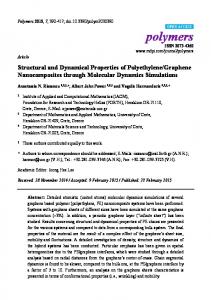
Fig. 1.— Dependence of the 2PIGG group velocity dispersion (left) and the group size (right) on redshift. The solid lines are third-order polynomial fits. [See the electronic edition of the Journal for a color version of this figure.]

groups which should be taken into account before attempting to derive their physical and morphological properties. For example, an outcome of the above group-finding algorithm is the increase with redshift of both the velocity dispersion and the projected size of the candidate groups. Such a systematic effect was also found in the Ramella et al. (2002) group catalog by Plionis et al. (2004). In Figure 1 we present the group velocity dispersion and a measure of their projected size as a function of group redshift (for groups with membership nm  4). The group projected size, related to the virial radius, is found by "

r¼

nm m 1 X nm (nm  1) nX 1 2 D tan (cij
ij ) i¼1 j¼iþ1 L

#1 ;

ð1Þ

where DL is the luminosity distance of the group within the concordance cosmological model (  ¼ 0:7, m ¼ 0:3, h72 ¼ 0:72),
ij is the angular (i; j)-pair separation, and cij is an average galaxy pair weight that takes into account the variable 2dFGRS incompleteness (in angular, redshift, and magnitude limit space). The individual galaxy weights are taken from Eke et al. (2004). Note that the above measure of the size is significantly smaller than the maximum group galaxy-pair separation, rmax . A strong redshift dependence is evident in Figure 1. The larger velocity dispersion of high-z groups could be possibly attributed to the fact that we tend to observe at large redshifts only the richest groups (due to the flux-limited nature of the 2dFGRS). However, the fact that the projected group size and velocity dispersion increase monotonically with redshift, while the large- and high-v groups are not found at lower redshifts, can be attributed only to the group identification method (for a thorough discussion of z-dependent effects of the FOF algorithm, see Frederic [1995] and Diaferio et al. [1999]). Therefore, the probability that the groups found are true dynamical entities decreases with increasing redshift, but even if the high-z groups are real (but contaminated) entities, they would constitute a different family of cosmic structures than the lower-z ones. One can attempt to take into account such systematic biases by applying the same group-finding algorithm on N-body simulations, the results of which can then be used to calibrate the statistical results based on the real data (e.g., Eke et al. 2004).

However, since in this study we are interested in deriving the physical characteristics of the observed groups, we attempt to quantify and minimize the various systematic biases. To this end, we also limit the 2PIGG sample to within a redshift of z ’ 0:08, a limit within which the density of groups (estimated in equalvolume shells) is roughly constant, as can be seen in Figure 2. We are finally left with 1948 nm  4 2PIGG groups, out of which 1788 have velocity dispersion estimates from Eke et al. (2004). 3. GROUP PROJECTED AND INTRINSIC SHAPES We derive the group projected axial ratio, q, by diagonalizing the two-dimensional inertia tensor (e.g., Carter & Metcalfe 1980), which fits the best ellipse on the projected discrete distribution of galaxy group members. In Figure 3 (left) we present the group median axial ratio as a function of group membership (circles).

Fig. 2.— Group space density as a function of distance, estimated in equal volume shells. The straight line delineates the range where the density is roughly constant. The error bars are 2  Poisson uncertainties. [See the electronic edition of the Journal for a color version of this figure.]

772

PLIONIS, BASILAKOS, & RAGONE-FIGUEROA

Vol. 650

Fig. 3.— Left: Correlation between the 2PIGG group richness (nm ) and their median projected axial ratio (circles). The solid line represents the expected distribution due to sampling effects (see text). Broken lines are the 33% and 67% quartiles of the corresponding distribution. Right: Distribution of axial ratios of 2PIGG groups with 19
nm
25 (histogram) and the corresponding Monte Carlo prolate (solid line) and oblate (dashed line) groups. The insert shows the correction factor with which we need to divide the raw group axial ratios in order to take into account the discreteness bias. [See the electronic edition of the Journal for a color version of this figure.]

An interesting trend is apparent with q increasing with increasing nm , while it appears that for nm k 25 the value of q converges to a final value of 0.56. We have verified that this correlation is not due to the increase with redshift of the group-linking volume, which induces the systematic trend seen in Figure 1. 3.1. Sampling Effects Discreteness effects have been found to affect the group shapes by artificially increasing ellipticities with decreasing sampling (Paz et al. 2006). We therefore ask the question what would the mean axial ratio of groups be, having intrinsic flattening that of the richest 2PIGG groups (i.e., q ’ 0:56, nm  25), when sampled with a smaller number of points? To answer this question we use Monte Carlo simulations to construct a large number (Nsim ¼ 30; 000 for each nm ) of spheroidal three-dimensional groups having a Gaussian distribution of intrinsic axial ratios, , which we then sample with nm random points. The mean and variance of the Gaussian is chosen, using a trial and error method, such that the corresponding median projected axial ratio, at the limit of dense sampling, is compatible with that of the richest 2PIGG groups. This is accomplished for a prolate or oblate spheroidal model, with hi ’ 0:47 and hi ’ 0:20, respectively, while  ’ 0:20 for both. Note that since the Gaussian is bounded between 0

1, different values of  can indeed affect the resulting median projected group axial ratio. Then each group is randomly oriented with respect to the line of sight, the group members are projected on a surface and the projected axial ratio is measured. The outcome of the simulations give for nm k 20 a median value of q ’ 0:54þ0:05 0:04 (showing that a sampling of 20 points per spheroid is adequate to recover the input axial ratio). The complete run as a function of nm can be seen as the continuous line in Figure 3 (left), from which it is evident that the 2PIGG nm -q correlation (circles) is reproduced exactly (using either the prolate or oblate model for the Monte Carlo groups). However, the distribution of the projected 2PIGG axial ratios was found to be in relatively good agreement only with that corresponding to the Monte Carlo prolate groups. For example, in the right panel of Figure 3 we plot the axial ratio distribution of 2PIGG groups with 19
nm
25 (histogram) and of the cor-

responding Monte Carlo groups for the two spheroidal models, prolate and oblate (continuous and dashed lines, respectively). This proves beyond any doubt that discreetness effects are the cause of the observed nm -q correlation and that the 2PIGG axial ratio distribution is more consistent with that of a prolate rather that an oblate three-dimensional model. Therefore, this analysis, which serves to clarify the effects of sampling on the projected group shape, also hints on the intrinsic morphology of the 2PIGG groups, which is formally derived in x 3.2. In the insert of the right panel of Figure 3, we plot the correction factor, fc , derived from this analysis with which we need to divide the raw group axial ratios in order to neutralize the discreteness bias discussed before. Although we correct accordingly all the group raw axial ratios, we use the richest (nm  10) 2PIGG groups, for which the discreteness correction is relatively small, to determine their intrinsic group shape distribution. We also put an upper limit to nm (=30), in order to exclude from our morphological analysis clusters of galaxies, which may have a different dynamical history and thus a different shape distribution (for cluster shapes, see Basilakos et al. [2000] and references therein). 3.2. Recovering the Intrinsic Axial Ratio Distribution An interesting question is whether the group three-dimensional shape distribution can be inferred from the projected one. This is an inversion problem for which, under the assumption of random group orientation with respect to the line of sight and of purely oblate or prolate spheroidal shapes, there is a unique inversion. The problem is described by a set of integral equations, first investigated by Hubble (1926) and given by Sandage et al. (1970) f (q) ¼

1 q2

Z 0

Z f (q) ¼ q 0

2 Nˆ p ( ) d

q

(1  q2 )1=2 (q2   2 )1=2 Nˆ o () d

q

(1 

q2 )1=2 (q2

 2 )1=2

;

prolate;

ð2Þ

;

oblate;

ð3Þ

where Nˆ o ( ) and Nˆ p ( ) are the intrinsic oblate and prolate axial ratio distributions, respectively, and f (q) is the corresponding

No. 2, 2006

MORPHOLOGY AND DYNAMICS OF 2dFGRS GROUPS

773

Fig. 4.— Left: Projected halo axial ratio distribution (circles) and the smooth fit from the nonparametric kernel estimator (solid line). Center and right: Comparison of the inverted intrinsic halo axial ratio distribution (solid line) with the distribution of ‘‘average’’ spheroidal fits to the three-dimensional halos (histograms) for either the prolate (center) or the oblate (right) models. [See the electronic edition of the Journal for a color version of this figure.]

projected distribution. The continuous function f (q) is derived from the discrete axial ratio frequency distribution using the socalled kernel estimators (for details, see Ryden [1996] and references therein). Although we do not review this method, we note that the basic kernel estimate of the frequency distribution is defined as N
q  q  1 X i K ; fˆ (q) ¼ Nh i h

ð4Þ

function where qi are the group axial ratios and K(t) is the kernel R (assumed here to be a Gaussian), defined so that K(t) dt ¼ 1, and h is the ‘‘kernel width’’ that determines the balance between smoothing and noise in the estimated distribution. The value of h is chosen so that the expected value of the integrated mean square error between the true, f (q), and estimated, fˆ (q), distributions is minimized (e.g., Vio et al. 1994; Tremblay & Merritt 1995). Inverting then the above equations gives us the distribution of true axial ratios as a function of fˆ (q) (e.g., Fall & Frenk 1983) ! 2 1=2 Z  ˆ 2(1   ) d dq f ; ð5Þ Nˆ o ( ) ¼ q ( 2  q 2 )1=2  0 dq and 2(1   2 )1=2 Nˆ p ( ) ¼ 

Z

 0

d  2 ˆ dq q f ; 2 dq (  q 2 )1=2

ð6Þ

where fˆ (0) ¼ 0. Integrating numerically equations (5) and (6), allowing Nˆ p (  ) and Nˆ o ( ) to take any value, we can derive the inverted (three-dimensional) axial ratio distributions. If groups are a mixture of the two spheroidal populations or they are triaxial ellipsoids, there is no unique inversion (Plionis et al. 1991). However, all may not be lost, and although the exact shape distribution may not be recovered accurately, one could possibly infer whether the three-dimensional halo shapes are predominantly more prolateor oblate-like. 3.3. Testing the Method with N-Body Simulations Here, we attempt to investigate the accuracy of the shape inversion method when the intrinsic three-dimensional shape distribution is not that of pure spheroids. To this end we use GADGET2 (Springel et al. 2005) to run a large (L ¼ 500 h1 Mpc, NP ¼

5123 particles) N-body (DM only) simulation of a flat low-density cold dark matter model with a matter density m ¼ 1   ¼ 0:3, Hubble constant H0 ¼ 72 km s1 Mpc1, and a normalization parameter of 8 ¼ 0:9 The particle mass is mP  7:7 ; 1010 h1 M , comparable to the mass of one single galaxy. The halos are defined using a FOF algorithm with a linking length given by l ¼ 0:17hni1/3, where hni is the mean density. This linking length corresponds to an overdensity ’330 at the present epoch (z ¼ 0). We use intermediate-richness halos with 6 ; 1013 h1 M
Mh
8 ; 1013 h1 M , for which there are more than 700 particles per halo and which, therefore, are free of discreteness effects. The total number of such halos is 2610. Dark matter halo shapes are quantified using the so-called triaxiality index ( Franx et al. 1991), defined as T ¼ (a 2  b2 )/ (a2  c 2 ), where a, b, and c are the major, intermediate, and minor halo axes of the best-fit ellipsoid, respectively, which has limiting values of T ¼ 1 (prolate spheroid) and T ¼ 0 (oblate spheroid). Our results, which are in agreement with other studies, show that the fraction of halos with pronounced prolateness (i.e., large T ) is significantly higher than that of oblate-like halos. Overall, we obtain from our simulated halos that hT i ’ 0:73. We now project into two-dimensions the distribution of halo particles and determine their projected axial ratios following the same procedure as in the real group data. In Figure 4 (left) we present the discrete and continuous f (q) distributions of the projected in two-dimensional halo axial ratios. In the central and right panels we present the inverted three-dimensional axial ratio distributions (solid lines) for the prolate and oblate models, respectively. It is evident that the inverted oblate-model distribution is unacceptable due to the many negative values (at large  ), while the opposite is true for the prolate-model distribution. As a further test we plot as histograms the intrinsic axial ratio distribution of the ‘‘average’’ prolate or oblate spheroidal fits to the three-dimensional halos. These fits are realized by estimating the corresponding axial ratios by p ¼ (b þ c)/2a and o ¼ 2c/(a þ b). It is evident that the purely oblate model fails miserably to even come close to the inverted distribution, while the prolate model fits relatively well the corresponding inverted three-dimensional prolate-model distribution. These results are in accordance with the intrinsic halo shapes determined in threedimensions, which were found to have a higher prolateness, as discussed previously. We therefore conclude that applying the previously discussed inversion method to observational data we can infer, even in the

774

PLIONIS, BASILAKOS, & RAGONE-FIGUEROA

Fig. 5.— Left : 2PIGG projected group axial ratio distribution (circles) and the smooth fit from the nonparametric kernel estimator (lines), for the discreteness corrected case ( filled circles and solid line) and the uncorrected case (open circles and dashed line). Center and right: Inverted intrinsic halo axial ratio distribution for the prolate (center) and the oblate (right) cases. [See the electronic edition of the Journal for a color version of this figure.]

still present (between z ’ 0 and 0.08 the average values of v and r increase by 50%). In order to statistically correct for this bias, we fitted third-order polynomial functions, V (v ; z) and S(r; z), to the data (Fig. 1, solid curves) and then corrected the raw v and r values by weighting them with V (v ; 0)/V (v ; z) and S(r; 0)/S(r; z), respectively. However, we also present results for the very local volume (z
0:03), which apparently is unaffected by the redshift dependent bias (see Table 1). Because of the discreteness effects quantified in x 3.1, there is also an enhancement of the projected group size, r, especially at small nm (e.g., we find a 18% increase of the projected size for groups with nm ¼ 4). For the velocity dispersion case we sample a Gaussian velocity distribution with nm , and we find a generally small effect (e.g., there is a 10% reduction of v for groups with nm ¼ 4). In Figure 6 we present the corrected (for all the above biases) group velocity dispersion and size as a function of redshift for our z
0:08 sample. It is evident that the strong dependence on redshift has been eradicated, and although the individual values of velocity dispersion and size may diverge from the intrinsic values, the overall population statistics should be correct. After applying the above corrections to the group velocity dispersion and size, we can estimate their virial mass and crossing time by

event of triaxial ellipsoidal halo shapes, the dominance of prolate or oblate-like three-dimensional shapes, if such does exist. 3.4. 2PIGG Intrinsic Shape In Figure 5 (left) we present the raw and discretenesscorrected projected axial ratio distributions for the 2PIGG groups with 10
nm
30 (circles) with their Poisson 1  error bars, while the lines show the continuous fits, f (q). The median discreteness-corrected axial ratio is q ¼ 0:55  0:08, while the uncorrected one is 0.51. In the central and left panels of Figure 5, we present the inverted intrinsic axial ratio distribution. The oblate model is completely unacceptable, since it produces many negative values (at large  ), while the prolate model fairs quite well, providing a roughly Gaussian intrinsic axial ratio distribution, with hi ’ 0:46 and  ’ 0:16 (which are also in very good agreement with the results of the Monte Carlo procedure of x 3.1). Also taking into account the N-body simulation analysis of x 3.3, our results imply that the 2PIGG group shapes is well represented only by that of triaxial ellipsoids with a pronounced prolateness, which is also in agreement with the previous analysis of poor groups ( Plionis et al. 2004) and compact groups (e.g., Oleak et al. 1995). 4. GROUP DYNAMICAL CHARACTERISTICS We are now interested in determining the typical size, velocity dispersion, crossing time, and virial mass of the 2PIGG groups. We remind the reader of the strong z-dependence of these parameters (Fig. 1), which is due to the group-finding algorithm. Although we have limited our analysis to 2PIGG groups within z ¼ 0:08, we observe that even within this z-limit, the previously discussed redshift dependant bias, although relatively weak, is

Mv ¼

3v2 Rv Rv ;  ¼ pffiffiffi ; G 3 v

where the group virial radius is Rv ¼ (/2)r (r given by eq. [1]). In Table 1 we present the median values of these parameters, as well as the maximum projected group intergalaxy separation (rmax ), for the bias-corrected sample (with z
0:08), for the very

TABLE 1 Median Dynamical Characteristics of 2PIGG Groups with 4
nm
30

z

No.

Correct Bias


0.08 ...................................
0.03 ...................................
0.08 ...................................
0.2 .....................................

1728 199 1728 6128

Yes No No No

v ( km s1) 150 157 188 257

ð7Þ

   

34 35 45 70

Mv (h1 72 M )

Rv (h1 72 Mpc)

rmax (h1 72 Mpc)

; ; ; ;

0.38 0.40 0.62 0.98

0.73 0.75 1.05 1.71

5.7 6.2 1.4 4.2

1012 1012 1013 1013

 ( yr) 1.5 1.3 1.9 2.2

; ; ; ;

109 109 109 109

Notes.— Characteristics are given for various cuts in redshift and for the redshift-bias-corrected and bias-uncorrected cases. We also present the uncorrected case for the very local volume (z
0:03), where the redshift bias is nonexistent.

Fig. 6.— Dependence of the corrected 2PIGG group velocity dispersion (left) and group size (right) on redshift.

Fig. 7.— The 2PIGG group virial radius (top left), the velocity dispersion (top right), the corresponding group crossing time (bottom left), and the group virial mass (bottom right) as a function of group richness (nm ). The open circles correspond to the raw values, and the filled circles correspond to the discreteness-corrected values. Note that here we also allow nm > 30 groups. [See the electronic edition of the Journal for a color version of this figure.]

776

PLIONIS, BASILAKOS, & RAGONE-FIGUEROA

local sample unaffected by the bias (z
0:03), as well as for two different redshift-limited samples, but with no corrections applied in order to appreciate the extend of the biases (note that the dominant correction is by far that of the redshift dependence). The comparison of these results yields that (1) the effect of correcting the z
0:08 groups is appreciable, while the corrected median values of Mv and Rv are about equal to those of the local sample (z
0:03), unaffected by biases, and (2) the effect is extremely large when using groups of any redshift (the uncorrected median values of Mv and Rv are respectively a factor of 8 and 3 larger than the corresponding corrected ones). When we now compare with determinations from other group catalogs, identified using similar FOF-based algorithms, we can appreciate the extent of the effect (see Table 1 of Mercha´n & Zandivarez 2005). The typical median values, resulting from different group catalogs that do not take into account this effect, are 1 M v ’ 5:5 ; 1013 h1 72 M and Rv ’ 1:4 h72 Mpc. In order to avoid such effects Tago et al. (2006) choose to use a constant in their redshift FOF-linking parameter. However, the decrease of the redshift selection function of the 2dF parent galaxy catalog implies that they select intrinsically different types of groups as a function of redshift (i.e., at higher redshifts they will tend to select more centrally condensed groups or the centers of clusters that have a high enough central density to survive the drop of the selection function at their distance). It is important to note that although the presented median values of the various dynamical group parameters are useful in order to compare with other studies, they are rather ill-defined, since we are mixing groups of different richness that could have distinct morphological and dynamical characteristics. Indeed, this is the case, and in Figure 7 we present the correlation between various dynamical and morphological group parameters with group ‘‘richness’’ (nm ). It is evident that there are very significant correlations of the group size, velocity dispersion, and virial mass with nm . A least-squares fit to the data corrected for the redshift bias and discreteness effects (nm  4) gives v ’ 4:83(0:26)nm þ 122(3) 1 km s1 Rv ’ 0:0212(0:0008)nm þ 0:254(0:007) 1 1 h72 Mpc log (Mv =1 h1 72 M ) ¼ 0:0416(0:0018)nm þ 12:36(0:02):

The above trends of the group projected size, velocity dispersion, and virial mass could be a natural consequence of the hierarchy of cosmic structures. It is also evident from Figure 7 that the 2PIGG groups have consistent crossing times, independent of the number of galaxy members, of 1.5 Gyr, which implies that the majority of them could be virialized systems (except probably for those formed within the last few billion years). Had we used instead of the virial radius the deprojected rmax value, we would have found a median crossing time of 3.8 Gyr, still significantly smaller than the age of the universe. 5. CONCLUSIONS Using Monte Carlo and N-body simulations, we have investigated the different biases that enter in the determination of the 2PIGG morphological and dynamical characteristics, and we have devised statistical correction procedures to recover their bias-free values. Within a redshift for which the 2PIGG groups have a roughly constant space number density (z
0:08), we derived the average morphological and dynamical characteristics (size, velocity dispersion, virial mass, and crossing times), which we find to be significantly smaller than those of other recent studies, precisely because we have taken into account the redshift-dependant bias. Within z
0:08, the median value of the group virial mass, virial 1 radius, and crossing time is 6 ; 1012 h1 72 M , 0:4 h72 Mpc, and 1.5 Gyr, respectively. Assuming that groups constitute a homogeneous spheroidal population, we numerically invert the projected, discretenessfree axial ratio distribution to obtain the corresponding intrinsic one. The only acceptable model is that of a prolate, or a triaxial with pronounced prolateness, distribution with a mean axial ratio of  ’ 0:46 and a dispersion of 0.16. We have also found that there is a correlation of the size and the velocity dispersion with the number of group members, which is probably a natural outcome of the hierarchy of cosmic structures.

C. Ragone-Figueroa acknowledges financial support by the Latin AmericanYEuropean Network for Astrophysics and Cosmology (LENAC) network and thanks the Instituto Nacional de ´ ptica y Electro´nica ( INAOE) for its hospitality. We Astrofı´sica, O also thank the referee, T. Goto, for useful suggestions.

REFERENCES Allgood, B., Flores, R. A., Primack, J. R., Kravtsov, A. V., Wechsler, R. H., Kasun, S. F., & Evrard, A. E. 2005, ApJ, 629, 781 Faltenbacher, A., & Bullock, J. S. 2006, MNRAS, 367, 1781 Lee, B. C., et al. 2004, AJ, 127, 1811 Bahcall, N., et al. 2003, ApJS, 148, 243 Lopes, P. A. A., de Carvalho, R. R., Gal, R. R., Djorgovski, S. G., Odewahn, Basilakos, S., Plionis, M., & Maddox, S. J. 2000, MNRAS, 316, 779 S. C., Mahabal, A. A., & Brunner, R. J. 2004, AJ, 128, 1017 Basilakos, S., Plionis, M., & Rowan-Robinson, M. 2001, MNRAS, 323, 47 Mercha´n, M. E., & Zandivarez, A. 2002, MNRAS, 335, 216 Berlind, A. A., et al. 2006, ApJ, submmitted, (astro-ph /0601346) ———. 2005, ApJ, 630, 759 Carter, D., & Metcalfe, N. 1980, MNRAS, 191, 325 Oleak, H., Stoll, D., Tiersch, H., & MacGillivray, H. T. 1995, AJ, 109, 1485 Cooray, R. A. 2000, MNRAS, 313, 783 Paz, D. J., Lambas, D. G., Padilla, N., & Mercha´n, M. 2006, MNRAS, 366, 1503 de Lapparent, V., Geller, M. J., & Huchra, J. P. 1991, ApJ, 369, 273 Plionis, M., Barrow, J. D., & Frenk, C. S. 1991, MNRAS, 249, 662 de Theije, P. A. M., Katgert, P., & van Kampen, E. 1995, MNRAS, 273, 30 Plionis, M., Basilakos, S., & Tovmassian, H. 2004, MNRAS, 352, 1323 Diaferio, A., Kauffmann, G., Colberg, J. M., & White, S. D. M. 1999, MNRAS, Plionis, M., Valdarnini, R., & Jing, Y. P. 1992, ApJ, 398, 12 307, 537 Ramella, M., Geller, M. J., Pisani, A., & da Costa, L. N. 2002, AJ, 123, 2976, Eke, V. R., et al. 2004, MNRAS, 348, 866 Ryden, S. B. 1996, ApJ, 461, 146 Fall, M., & Frenk, C. S. 1983, AJ, 88, 1626 Sandage, A., Freeman, K. C., & Stokes, N. R. 1970, ApJ, 160, 831 Franx, M., Illingworth, G., & de Zeeuw, T., 1991, ApJ, 383, 112 Sathyaprakash, B. S., Sahni, V., Shandarin, S. & Fisher, K. B. 1998, ApJ, 507, L109 Frederic, J. J. 1995, ApJS, 97, 259 Sereno, M., De Filippis, E., Longo, G., & Bautz, M. W. 2006, ApJ, 645, 170 Gal, R. R., de Carvalho, R. R., Lopes, P. A. A., Djorgovski, S. G., Brunner, Springel, V. 2005, MNRAS, 364, 1105 R. J., Mahabal, A., & Odewahn, S. C. 2003, AJ, 125, 2064 Tago, E., et al. 2006, Astron. Nachr., 327, 365 Goto, T., et al. 2002, AJ, 123, 1807 Tremblay, B., & Merrit, D. 1995, AJ, 110, 1039 Hubble, E. P. 1926, ApJ, 64, 321 Valdarnini, R., Ghizzardi, S., & Bonometto, S. 1999, NewA, 4, 71 Jaaniste, J., Tago, E., Einsato, M., Einsato, J., Andernach, H., & Mueller, V. Vio, R., Fasano, G., Lazzarin, M., & Lessi, O. 1994, A&A, 289, 640 1998, A&A, 336, 35 Zeldovich, Ya. B., Einasto, J., & Shandarin, S. 1982, Nature, 300, 407 Jing, Y. P., & Suto, Y. 2002, ApJ, 574, 538