Research Corporation (SRC) under contract No. 91-DJ-147. This paper presents ...... (ICCD-91), Oct. 1991. 21] NCR ASIC Data Book, NCR Corporation, 1989.
Move Frame Scheduling and Mixed Scheduling-Allocation for the Automated Synthesis of Digital Systems y Mehrdad Nourani and Christos Papachristou Department of Computer Engineering Case Western Reserve University Cleveland, OH 44106
Abstract
This paper presents new algorithms for the scheduling and allocation phases in high-level synthesis under time and resource constraints. This is achieved by formulating these problems in terms of Liapunov's stability theorem using a transformation technique between the design space and the dynamic system space. These algorithms are based on moves in the design space, which correspond to the moves towards the equilibrium point in the dynamic system space. The scheduling algorithm (MFS) takes care of mutually exclusive operations, loop folding, multicycle operations, chained operations and pipelining (structural and functional). The mixed scheduling-allocation algorithm (MFSA) can handle all of the above scheduling applications as well as simultaneously performing allocation of functional units, registers and interconnects while minimizing the overall cost.
1 Introduction
High-level synthesis deals with the automatic design of register transfer level (RTL) implementations of digital systems from behavioral descriptions. A behavior may represent a general purpose computer, an application speci c system (ASIC), or a combination of them. Behavioral synthesis is normally achieved in two basic steps: 1) Data path synthesis (operation scheduling and hardware allocation), and 2) Control path design. In the scheduling phase, operations are assigned to the appropriate control steps. The allocation phase speci es the design at a register transfer level by assigning operations into the hardware components. Operation scheduling determines the hardware cost-speed tradeo�s of a design. The simplest way to perform scheduling is to relegate the task to the user to explicitly de ne the parallelism of the design such as in the SLICE system [1]. The FACET system, presented in [2], used ASAP schedule for nding near optimal solution. Conditional deferment methods, such as in [3], were based on the fact that if the operation concurrency is higher than the number of available units, those operations should be postponed. List scheduling techniques, such as in [4], sort and then schedule operations in topological order based on priorities (or mobilities), are more complex class of algorithms. The fact that decisions at higher levels of synthesis (i.e. allocation) may dominate the results produced by an independent scheduling phase was a motivation to develop another class of methods in which these two phases are interdependent. MAHA [5] attempts to perform scheduling and allocation in parallel by allocating hypothetical average functional units during the list scheduling phase. HAL [6] uses a stepwise re nement technique which uses force-directed scheduling assuming single-function units. A simulated annealing based algorithm was used to perform scheduling and allocation together in one process [8]. Some researchers [3][11][9][10] use linear programming formulation to develop scheduling and allocation algorithms. Neural network-based models such as [12]have been recently attempted. y This work was partially supported by the Semiconductor Research Corporation (SRC) under contract No. 91-DJ-147
This paper presents new algorithms for scheduling and mixed scheduling-allocation process in high level synthesis. The main contribution of our method is in the following: 1. A new fast scheduling method, Move Frame Scheduling (MFS) which performs guided search in the huge state space of schedules, driven by Liapunov's stability theorem. 2. A new fast scheduling-allocation method, Move Frame Scheduling-Allocation (MFSA), which extends the guiding mechanism of MFS to search the scheduling and allocation spaces simultaneously. 3. The methods can be applied to di�erent synthesis aspects under time and resource constraints. The main advantage of our methods over existing scheduling and allocation algorithms is in running time. Two speci c characteristics provide this important advantage. First, the main decisions to schedule or allocate an operation in data ow graph (DFG) are made within a relatively small 2-dimensional frame. Second, our methods do not su�er from the size explosion problem for variables and/or constraints as some methods (e.g. linear programming-based) do. Furthermore, based on the Liapunov's theorem, we use the Liapunov (energy) function as the guiding mechanism to approach optimal solution while avoiding the probablistic exploration and tunning problems in some energy-based approaches such as annealing and neural networks. This paper is organized as follows: Section 2 reviews the transformation technique and stability problem. Sections 3 and 4 describe the MFS and MFSA methods, respectively. Section 5 extends MFS and MFSA to include a number of important synthesis aspects. The experimental results are shown in section 6. Finally, concluding remarks are in section 7.
2 The Synthesis Problem Transformed to a Stability Problem 2.1 Transformation Technique
The basic idea is to use the similarities between the synthesis problem in computer engineering and the stability problem in control theory. In this analogy, system, stability and equilibrium point have the same notion as algorithm, convergence and optimal solution, respectively. The mathematical proof for correctness of this transformation is beyond the scope of this article. The details can be found in [13] and [14].
2.2 Stability Concept and Liapunov Theorem
Based on [15] a system is asymptotically stable at the equilibrium point if and only if a trajectory beginning in a suitable neighborhood of the equilibrium point tends to the equilibrium point as the time passes. The problem of determining whether or not a system is stable is fundamental in all control system design. For non-linear systems the Liapunov's theorem has the greatest potential for investigating stability in such systems. This theorem is more a principle than a technique. Intuitively speaking, if the time rate of change of the energy E of an isolated system is negative for every possible state X of the system, except for a single equilibrium state Xe , then the
energy will continually decrease until it nally assumes its minimum. The generalization of this concept was considered by M. A. Liapunov. He expressed his idea by the following theorem: A dynamic system described by the discrete time vector equation X (k + 1) = A(k) � X (k) (k = 0; 1; 2; ���) is stable if and only if there exists a scalar Liapunov function V (X ) : Rn ! R+ with the following properties: 1. V (X (k)) > 0 when X (k) 6= Xe. 2. V (X (k + 1)) ? V (X (k)) < 0 when X (k) 6= Xe . 3. V (X (k)) = 0 when X (k) = Xe. 4. limkX k!1 V (X ) = 1. The main practical point of this theorem is that if such a function V (X ) exists, then it guarantees that the system is stable and if we let time grow, by selecting an appropriate movement mechanism (i. e. make V (X ) decreasing monotonically) the system tends towards, and nally reaches, the equilibrium point. Complete proof of this theorem for different cases (discrete or continuous time) can be found in many of control theory books such as [15].
2.3 New Formulation of Synthesis Problem
To use Liapunov's theorem, we must rst formulate the synthesis problem as a system whose behavior can be expressed by the vector equation X (k + 1) = A(k) � X (k). Given a DFG for each operation Oi (1 � i � l), consider a 2-dimensional placement (grid) table shown in Figure 1. One dimension represents the number of control steps and the other shows the instances of functional units (hardware modules). In a scheduling algorithm, the functional units are assumed to be single function operators, while in a simultaneous scheduling-allocation algorithm they are also allowed to be multifunctional units (ALU's). This assumption is due to the fact that in the scheduling phase the concurrency of similar operations is an important factor, while in the allocation phase merging di�erent operations can signi cantly decrease the overall ALU cost. In Figure 1, the horizontal coordinate represents the number of functional units (FU) of a speci c type, and the vertical coordinate shows the number of control steps. For example, the present position of operation Oi , denoted by Oip , shows that Oi is performed by the fourth functional unit of that type in the sixth control step. Note that because we normally have more than one type of functional units, the complete space will be a 3-dimensional space where the third dimension represents the type of FU's. Note that Figure 1 does not show this but Figure 2 shows a 2-dimensional representation of this 3-dimensional space for a typical example. We de ne Xe = ~0 as the equilibrium point (which is a dummy one in the synthesis problem because obviously ~0 = (0; 0) is not accessible). Let us assume that the system is stable, and let time grow. Then in a trajectory towards the equilibrium point, the present position of Oi , denoted by Oip , at time k (k-th step of the movement) is: Xi(k) = (xi;k ; yi;k )T . Similarly, the next position of Oi , denoted by Oin�, at time �k +1 �is: Xi (k +1) =�� (xi;k+1 ; y�i;k+1 )T . x a 0 xi;k where i;k+1 = i;k Assuming: yi;k 0 bi;k yi;k +1 ai;k and bi;k are two positive real numbers, we have: Xi(k + 1) = Ai (k) � Xi (k). If we join all of similar elements corresponding to all operations Oi (1 � i � l) in DFG, we will totally get: 0 XX1((kk ++ 1)1) =1A(k) � X (k0) where: X1 (k) 1 .. A, X (k) = @ ... A, X (k + 1) = @ . Xl (k) 0 A1(kX) l(k���+ 1) 0 1 � � .. A and 0 = 0 0 . A(k) = @ ... . ��� 0 0 0 ��� Al (k)
2.4 Liapunov Function in Synthesis Problems
So far we have formulated the general synthesis problem so as to apply Liapunov's theorem. Application of this theorem involves nding a function satisfying those basic properties mentioned in section 2.2. Unfortunately, there is no standard method for nding such a function. Moreover, a Liapunov function may not be unique. Di�erent Liapunov functions will produce di�erent performances, and consequently di�erent results. The general role of the Liapunov function in MFS and MFSA is the same as the energy function in annealing and neural network based approaches. In fact, some researchers in the latter area call their energy function Liapunov function. Scheduling (and allocation) in MFS (and MFSA) is accomplished by moves in the 2-dimensional grid space. The direction of moves and the moves themselves should satisfy the Liapunov theorem criteria. The Liapunov function is used not only to guarantee approaching to the equilibrium point, but also to specify the direction towards it. The rst role is guaranteed if the energy function satis es those four properties. However, the problem constraints and speci cations determine which direction is more desirable.
3 Move Frame Scheduling Algorithm (MFS)
Our goal, in introducing MFS as an independent scheduling algorithm, is twofold. First, the scheduling process is less complicated and easier to describe. Moreover, in many practical applications we need to do the scheduling rst. Second, we want to show that MFS itself has enough credibility as an independent scheduling algorithm for producing a balanced schedule for any desirable allocation process that follows.
3.1 Liapunov Function Used in MFS
When we schedule an operation under time constraints, we should not waste any control steps. In other words, the Liapunov (energy) function should make sure that control step t is selected before t +1, if possible. Assume that maxj number of functional units of type j (denoted by FUj;1 ; FUj;2 ; ��� ; FUj;maxj ) are available. Then, to select control step t before t + 1, it is su�cient to assign a lower energy value for position (FUj;maxj ; t) than position (FUj;1 ; t +1). This relation should be valid for any FU and any control step. Based on requirements, consider this function: V (X (k)) = Pl these ( x + n � yi;k ) where n = Maxfmaxj g; 1 � j � numi;k i=1 ber of types of FU's. maxj may be speci ed by the user as a resource constraint or can be set to a presummed big number as the upper bound. By a similar argument, P we can easily show that the function: V (X (k)) = li=1 (cs � xi;k + yi;k ) where cs is an upper bound for total number of control steps, is a Liapunov function which can be applied to scheduling under resource constraints. This function selects a position in control step t + 1 performed by an existing FU instead of adding a new FU in control step t. For each operation Oi (1 � i � l), the next position must be closer to the equilibrium point. The closeness will be interpreted by the Liapunov function. It is trivial to show that properties (1), (3) and (4) are held. To satisfy property (2) we must have : xi;k+1 < xi;k and yi;k+1 < yi;k . This means that the next position of each operation should be to the left and/or above of its present position. Moreover, the next position should satisfy the data dependency constraints.
3.2 Scheme and Example
To generate a balanced schedule (minimum concurrency) under xed time constraint, MFS proceeds in the following four steps: � Step 1: Find ASAP (As Soon As Possible) and ALAP (As Late As Possible) schedules, within the given num-
ber of control steps, to specify the time frame for each operation. Figure 2(a) shows these schedules. � Step 2: Select an arbitrary ordering of di�erent types of FU's and do all the subsequent phases in this order. { Set the maximum number of di�erent types of FU's, maxj (1 � j � number of types) to the numbers given by the user as the hardware constraints. For example, if the user requires up to 4 adders then max+ = 4. If they are not given by the user, nd the maximum number of FU's in ASAP and ALAP schedules and select them as the upper bound. { Calculate the mobility � for each operation: mob[Oi] = ALAPc?step[Oi ] ? ASAPc?step[Oi ] { Determine the priorities of operations in ALAP schedule based on their mobilities. The rule is very simple: If mob[p] < mob[q] then p has more priority than q. Priority determination starts from the rst control step and will cover all control steps in ALAP. Ties will be broken arbitrarily. � Step 3: Construct ASNAP (As Soon and Near As Possible) and ALFAP (As Late and Far As Possible) tables. Brie y, the ASNAP and ALFAP tables, specify a 2-dimensional frame (rectangle) for moving each operation individually and independently. For an operation of type j , this frame is speci ed by [1; cs] and [1;maxj ]. � Step 4: Schedule each operation in the order of its priority by the following process: { Determine the Primary Frame (PF): This is a 2dimensional frame for each operation restricted by its place in ASNAP and ALFAP tables. { Determine the Redundant Frame (RF): Since we do not know how many of them we really need, we consider a variable to show the current number of FU's (currentj ). We set this variable to dNj =cse where Nj is the total number of operations of type j in DFG and cs is the total number of control steps. At each step the frame de ned by [ASAPc?step; ALAPc?step] and [currentj +1; maxj ] represents the redundant frame. { Determine the Forbidden Frame (FF): We must exclude those positions whose control steps are less than or equal to the predecessors (of Oi ) control step, in order to satisfy the data dependency constraints. These excluded positions form the forbidden frame. { Determine the Move Frame (MF): This is the valid frame in which an operation can be scheduled. For each operation we have: MFOi = PFOi ? (RFOi + FFOi). Note that this equation represents a set relation between the frames because each frame is really a set of positions. Figure 2, (a) and (b), illustrates the above frames for a typical operation r of type j . In this gure, we assume that operation r has two predecessors, namely K1 and K2, and the current number of functional units of type j at that step is two (currentj = 2). These oper-� ations have already been assigned to positions K1 and K2� in previous steps (X shows other occupied positions). { Select one of the available positions in MF (move frame) which has the smallest Liapunov value and assign operation Oi in it. If there is no valid position for Oi (i.e. MFOi is empty or fully occupied), increase currentj by one and then do a local rescheduling by going back to step 3. For the � The mobility is the di�erence in control steps between the scheduled places of an operation in ALAP and ASAP schedules, respectively. Many researchers such as [4] and [6] have already used this notion.
example shown in Figure 2, the best position in MF to assign operation r will be r� . Analysis of MFS shows that the algorithm runs in O(l3 ) in the worst case, where l is total number of operations.
4 Move Frame Scheduling-Allocation Algorithm (MFSA)
Many researchers [7-9] believe that because of the tight interaction between scheduling and allocation, a simultaneous algorithm has a better chance to capture the global optimal solution. However, such algorithms may be slower and more complex. They usually su�er from size explosion (e.g.linear programming based), probablistic nature (e.g. simulated annealing) or unreliable approximations for nonlinear objective functions. MFSA is an algorithm in which the scheduling, allocation and data path optimization processes interact with each other by means of a complex Liapunov function. The Liapunov function in MFSA is capable of selecting and optimizing di�erent types of functional units (ALU's), optimizing multiplexers (or buses), registers and data path connections. As we will show shortly, although MFSA is a bit slower than MFS, the complexity of MFSA is the same as MFS because the 2-dimensional tables (search space) and general movement mechanism within the move frame for operations remain unchanged. The Liapunov function in MFSA is nonlinear and complex but we are not going to optimize it. In fact, similar to MFS, this function is used as an evaluation tool to guide the movement in the search space.
4.1 Liapunov Function Used in MFSA
MFSA uses the same 3-dimensional space (combination of 2-dimensional tables) as MFS explained in section 3. So, the behavior of the system can still be represented by the vector equation: X (k + 1) = A(k) � X (k). To have the necessary information for multiplexer (MUX) and register (REG) optimization, we should annotate the input signals (input variables) of each operation, together with its name in the DFG and other tables. As we will show shortly, these signals play a major role in the Liapunov function and MFSA algorithm. The following important rules will be considered in the new Liapunov function: � In time constrained problems, control step t should be selected before t + 1, as explained in MFS. � When a new functional unit (called \ALU" in MFSA) is used for performing an operation, its cost should be added to the incremental ALU cost up to that iteration. The cost of an existing ALU, previously used to perform other operations, is zero. � When the Liapunov function evaluates an ALU for assigning an operation, the input signals associated with all operations in that ALU should maximally share MUX inputs to minimize MUX cost. If we assume that each operation has at most two input signals, after assigning a new operation to an ALU it may share zero, one or two signals with other operations. � When the Liapunov function evaluates a speci c control step to assign an operation, the life span of its input signals (coming from its predecessors scheduled and allocated at previous iterations) can be determined. Thus, we can evaluate the e�ect of this selection to the cost of registers up to that point. Assume that the Liapunov function nds the best position for Oi in the 2-dimensional valid frame (MFOi frame) in kth iteration (i.e. kth time evaluation of appropriate time slots and ALU's). Let yi;j;k and xi;j;k denote the time slot (expressed in control steps) and ALU index of type j (index of ALU of type j when many ALU's of this type are available) chosen in kth iteration by the Liapunov function, respectively. Based on the above points and notations, consider this Liapunov function:
P
TIME + f ALU + f MUX + f REG ). V (X (k)) = li=1 (fi;j;k i;j;k i;j;k i;j;k fi;j;k represents the contribution of Oi in the Liapunov function when it is evaluated in the kth iteration. Recall that
in MFS, each operation can be only assigned to a functional unit of its type, e.g. an addition is always assigned to an adder (+), but in MFSA each operation can be assigned to di�erent functional units, e.g. an addition may be assigned to single or multifunction ALU's such as (+), (+?), (+ >) or (+? >) based on the cell library given by the user. Note also that all other operations scheduled and allocated in the previous iterations keep their contributions in the Liapunov function unchanged. Now, let's explain each term in V (X (k)) for a speci c operation Oi . For brevity, we will show the four terms involved in the function without their subscripts, i.e. f TIME , f ALU , f MUX and f REG : � f TIME = f TIME (yi;j;k ) = C � yi;j;k C is a constant that guarantees control step t is selected before t + 1 if it is possible. To guarantee this in iteration k (in which control step yi;j;k has been selected) we must satisfy: ALU + fmax MUX + fmax REG < C � (yi;j;k + 1) + C � yi;j;k + fmax ALU MUX REG fmin + fmin +f ALU + fmin MUX REG ALU MUX or: C > [fmax max + fmax ] ? [fmin + fmin + REG fmin ] The maximum and minimum values for f ALU ; f MUX ALU , f ALU , etc., will be determined and f REG , i.e. fmax min shortly when we describe each term. � f ALU = f ALU (xi;j;k ) When we use a new ALU, its cost should be added to the overall ALU cost. So, f ALU (xi;j;k ) = Cost(ALUj ) if ALU speci ed by xi;j;k has not already been used. Otherwise the cost of using an existing ALU is zero. ALU = Cost(ALUj ) and f ALU = 0. Clearly, fmax min MUX MUX �f =f (xi;j;k ; Si;j;k ) Si;j;k is the set of input signals of operations in the ALU speci ed by xi;j;k (xi;j;k th ALU of type j ). The term f MUX represents the possibility of signal sharing after adding the new operation in this ALU. In a straight forward design in which each ALU has two multiplexers (MUX 1 and MUX 2 ) feeding the ALU input signals, we have: f MUX = f MUX (xi;j;k ; Si;j;k ) = 1 ) + Cost(MUX 2 )]? [Cost(MUXafter after 1 2 [Cost(MUXbefore ) + Cost(MUXbefore )], where subscripts before and after denote the multiplexer con gurations before and after adding operation Oi , respectively. Practically, the cost of a multiplexer with r data inputs and 1 output, denoted by Cost(MUXr ), is not a linear function of r. So, depending on the cell library used in the design : MUX = 2 � maxfCost(MUXr+1 ) ? Cost(MUXr )g fmax MUX = 0. where r = 1; 2; ��� and fmin � f REG = f REG (yi;j;k ; Pi;j;k ) Pi;j;k is the set of predecessors of operation Oi which have been scheduled and allocated in the previous iterations. When Oi is assigned to control step yi;j;k , the consuming time of signals generated by those predecessors (up to iteration k) will be yi;j;k . In other words, in a backward look at the partially constructed schedule (up to iteration k) the life spans of input signals of Oi (coming from predecessor nodes or registers) are determined. Assuming that Oi has at most two inputs, then zero, one or two registers are needed to store those signals until they are consumed by Oi . Obviously, REG = 2 � Cost(REG) and f REG = 0. fmax min If the user wishes to put more emphasis on optimizing one of the four factors participating in the Liapunov function (TIME, ALU, MUX and REG), he/she may consider a weighted Liapunov function as: fi;j;k = (wTIME � f TIME )+
(wALU � f ALU ) + (wMUX � f MUX ) + (wREG � f REG ), where wTIME ; wALU ; wMUX and wREG are weights based on the relative importance of each factor. wTIME = wALU = wMUX = wREG = 1 gives an overall optimizer without emphasising any particular factor. Similar to MFS, properties (1),(3) and (4) are clearly held. Property (2) is also satis ed if we consider a movement mechanism that moves Oi from (xi;j;k ; yi;j;k ) to (xi;j;k+1 ; yi;j;k+1 ) if and only if fi;j;k+1 < fi;j;k .
4.2 Scheme and Example
The MFSA generates an RTL (register transfer level) structure in the following steps: � Step 1, Step 2, and Step 3 are exactly the same as the rst three steps in MFS algorithm. As we have already pointed out, the only di�erence is that we record the input signals together with the operations when di�erent tables and frames are constructed in the process. � Step 4: Consider each operation in order of priorities as in MFS by the following process: { Determine all ALU's (i.e single or multifunction ALU of type j ) capable of performing operation Oi . { Determine the frames PFOi ;j , RFOi ;j , FFOi ;j and MFOi ;j for those ALU's found in the previous step. { Compute the Liapunov function values for each empty position in MFOi ;j . Then, select a position in this frame with the smallest associated Liapunov value and assign Oi to that position (xi;j;k th control step and yi;j;k th ALU) and update the function and tables. It is important to note that the Liapunov function in MFS is a static function. It assigns a xed value to each position in the tables or frames in the entire process. In MFSA, however, the Liapunov function is a dynamic function which is updated in each iteration based on the best con guration of the table (operations, input signals, multiplexers and registers) found in the previous iterations. The running time is also O(l3 ), the same order as in MFS. To show how other speci cations (other than those considered directly in the Liapunov function) can be handled in MFSA, we consider two design styles: 1. Conventional data path design style (unrestricted RTL structure). 2. Restricted design style which gives an RTL structure without a self loop around ALU's. This has been proven to be useful for having a self testable structure [18]. So, in this case no operation is allowed to be with its successors or predecessors within the same ALU.
5 Applications to Synthesis Problems 5.1 Conditional Statements
If-then-else and case statements cause branches in the DFG. Operations in di�erent branches are mutually exclusive, thus they can be executed on the same type of FU and scheduled into the same control step without increasing the required number of FU's. To take advantage of this observation, we remove all of the operations which are shared between branches except one of them. Obviously, those shared operations can be executed by the same FU.
5.2 Loops
The user should specify a constraint on the loop iteration time. This can be done by adding two more operations (addition and comparison or increment and comparison) into the DFG corresponding to the body of the loop. Then the operations bounded by the new DFG are considered within the constraint using MFS or MFSA.
For nested loops, the operations of the inner most loop are scheduled and allocated rst, relative to the local time constraint. When this is done, the entire loop is treated as a single operation with an execution time that is equal to the loop's local time constraint. This process is repeated for all loops until the outer most loop is scheduled and allocated. Loop unfolding by using functional pipelining is another way to handle loops. We will comment on this issue shortly.
5.3 Multi-Cycle Operations
The fact that di�erent operations have di�erent execution time, has been of concern in the literature. MFS and MFSA consider k-cycle operations as k consecutive single-cycle operations of di�erent types. To be able to run our methods on multi-cycle operations, we should consider the following modi cations: � All assumed k single-cycle operations must be scheduled in consecutive control steps because no delay is allowed during the execution of an operation. � Two k-cycle operations are concurrent if at least one of their k consecutive stages is concurrent. � If the di�erence of mobilities between two k-cycle operations is less than k, we will reverse the previous rule for priority determination because, in this special case, the operation with more mobility has always a better chance to use the empty positions. � As a rule for tie breaking, the operation with earlier predecessors (in terms of control steps), will get higher priority.
5.4 Chained Operations
Scheduling of consecutive data dependent operations in a single control step is called chaining. This feature is supported by our methods, MFS and MFSA, by considering the following extensions: � ASAP and ALAP schedules (and consequently the mobilities and priorities) are determined based on the given execution time of operations and the length of control step clock (T). � The Forbidden Frame (FF) which originally excludes the control steps of predecessors, should be changed to allow chaining.
5.5 Pipelining
The optimization of scheduling when we have pipelined behavior in synthesis is a very important issue according to recent developments in this area. Two simple and e�cient pipelining techniques (structural and functional) have been presented in the literature [6][16][17]. Both of these pipelining techniques are supported by our methods using simple modi cations.
5.5.1 Structural Pipelining
In structural pipelining, a modi ed schedule is obtained through the use of pipelined FU's, e.g. a two-stage pipelined multiplier, so that the operation instances are executed in an overlapping fashion. The extension of MFS and MFSA for structural pipelining is based on the fact that once any stage of a pipelined FU is empty, it is considered available. We then consider these modi cations: � Change multi-cycle operations (for which a pipelined FU's are available) to single-cycle operations of di�erent types. After this modi cation, di�erent operations represent di�erent stages of a multi-stage pipelined functional unit. � Run the algorithm on the new DFG considering the fact that di�erent stages of pipelined operations can be concurrent but must be scheduled in consecutive control steps.
5.5.2 Functional Pipelining
In functional pipelining we try to divide the DFG description (operations) into some partitions that can be performed concurrently. Successive partitions are streamed into the pipe so that di�erent instances are executed in an overlapping fashion. In loop unfolding application, each instance corresponds to a new initiation of the loop. For a given latency L, the operations scheduled into control step t + k � L (k = 1; 2; 3; ���) run concurrently, so we must balance the distribution of operations across all individual control steps. To consider functional pipelining we need the following process: 1. Given the DFG description (i.e. body of a loop), the time constraint for DFG (cs control steps) and latency L, consider a new DFG consisting of two instances with delay of L cycles in between. 2. Divide the new DFG into two partitions DFGp1 and DFGp2 . DFGp1 consists of all operations between control step 1 and d cs2+L e. Similarly, DFGp2 consists of all operations between control step d cs2+L e + 1 and cs + L. Clearly DFGdouble = DFGp1 [ DFGp2 . 3. Run the algorithm on DFGp1 , taking into account the time frame for operations belonging to Instance 2 by adding dummy operations if it is necessary. 4. Adjust the result of the previous step in order to get identical instances. To do this, we should add all operations which are in (Instance1) \ DFGp1 but not in (Instance2) \ DFGp1 . 5. Eliminate adjusted operations (added in previous step) from DFGp2 and run the algorithm on the remaining operations in DFGp2 .
5.6 Multiplexer Optimization
Term f MUX in the Liapunov function, explained in section 4, evaluates the contribution of operation Oi to the multiplexer cost. To consider multiplexer optimization, two 1 ) and Cost(MUX 2 ) terms in f MUX , i.e. Cost(MUXafter after should be evaluated under the best case of sharing for the input signals. Assuming that each operation has at most two inputs, MFSA uses a constructive algorithm which reads the set of operations assigned to a speci c ALU and their corresponding inputs and constructs two lists of input signals L1 and L2 such that jL1 j + jL2 j is minimum. Brie y, the algorithm rst assigns the non-commutative operations to the appropriate MUX's of an ALU and then checks two possibilities for arranging input signals for each commutative operation in L1 and L2 .
5.7 Interconnect Optimization
When some of the operations performed by ALUr are successors (or predecessors) of operations in ALUs , the connection lines carrying the data between ALUr and ALUs, and consequently the input lines to the multiplexers of these ALU's, can be shared unless there is a con ict between them (e.g. both predecessors of an operation are located in the same ALU). Line sharing for data transfer between ALU's has a 1 ) and Cost(MUX 2 ) secondary e�ect on Cost(MUXafter after MUX terms in f before the Liapunov function makes its nal decision.
5.8 Register Optimization
Term f REG itself, considers register optimization by nding the least number of registers saving signals required to perform operations within an ALU at that iteration. To nd this number, we use an expanded version of the activity selection algorithmy. This is a greedy algorithm capable y This algorithm is an extended version of the left edge algorithm used by many researchers such as [19].
of nding the best solution for one register in �(m) where m is the number of signals some of which are selected to
be saved in that REG. Brie y, the signal with the smallest death time is selected and if it is compatible (no time con ict) with other signals in the register it will be assigned to that register.
6 Experimental Results
The MFS and MFSA algorithms described in the previous sections have been implemented in C on a SUN SPARCSLC workstation. These methods can easily be integrated with any synthesis tool. Currently, they are some of the options for scheduling and allocation in our high level synthesis tool called SYNTEST [20] which produces a self-testable RTL structure from a behavioral description. If MFS is selected, it reads the initial behavior (DFG) and the user has to specify the constraints and speci cations (including total control steps, execution time for each type of operations, pipeline options and so on). Then MFS nds a balanced schedule under design constraints. If MFSA is selected, in addition to the above constraints and speci cations, the cell library (which may be restricted to some speci c types) and other limitation imposed to RTL structure (i.e. design styles explained before) should be prepared for the system. Then MFSA generates a schedule and its corresponding RTL structure while optimizing the overall cost. This section presents brief results for six design examples from the literature. Table 1 shows a summary of the design results produced by MFS for the above six examples. In the second column, \1" means all operations take one cycle and \2" shows only multiplication consumes two cycles. Also \C ", \F " and \S " in this column show the special feature of that design, i.e chaining, functional pipelining and structural pipelining, respectively. Note, the CPU time for all examples is less than 0.2 seconds on a SPARC station. The result of MFSA which is a simultaneous schedulingallocation algorithm are tabulated in Table 2. Style 1 is unrestricted RTL structure while style 2 is RTL structure without self loop around ALU's. Overall cost of RTL designs (in micron square) is based on a NCR library [21]. The CPU time for running MFSA is less than 0.4 seconds for these examples. The wall clock time is about three seconds. For comparison, we have estimated the overall RTL structure cost (in micron square) based on the NCR library [21]. Comparison between the presented methods in the literature [6][5][11] and the rst design style obtained by MFSA shows an improvement of 1 ? 5% for examples 3, 5 and 6, while for examples 1 it shows 4% overhead. However, direct comparisons with other methods are not possible because of the di�erence in cell libraries and speci cation of the design and unavailability of their complete RTL structure. On the other hand, design style 2 shows 2 ? 11% overhead compared to design style 1. This is due to the fact that in style 2, the method imposes more restrictions for merging operations and sharing input signals within ALU's [18][20].
7 Conclusion
In this paper, we have presented a new approach to data path synthesis under time or resource constraints which is suitable for computationally dense behaviors such as digital signal processors and other ASIC systems. An important feature of our method is that by applying the global stability concept of dynamic systems to the transformed problem of scheduling and allocation, the MFS and MFSA algorithms explore the search space in a guided and global fashion and produce optimal or near-optimal results for all of the examples attempted to date. Furthermore, the exibility of Liapunov's stability approach as a guiding mechanism of the MFS and MFSA algorithms was highlighted by supporting di�erent practical aspects of synthesis including mutually exclusive operations, loop folding, chaining, multi-cycle operations, pipelining and multiplexer and register optimization.
References
[1] T. Blackman et al., \The Slice compiler: Language and features," Proc. 22nd Design Automat. Conf., June 1985. [2] C. Tseng and D. P. Siewiorek, \FACET: A Procedure for the Automated Synthesis of Digital Systems," Proc. 20th Design Automat. Conf., June 1983. [3] P. Marwedel, \A new synthesis algorithm for the MIMOLA software system," Proc. 23rd Design Automat. Conf., July 1986. [4] B. M. Pangrel and D. D. Gajski, \Slicer: A state synthesizer for intelligent silicon compilation," Proc. IEEE Int. Conf. Computer Design (ICCD-87), Oct. 1987. [5] A. C. Parker et al., \ MAHA: A program for data path synthesis," Proc. 23rd Design Automat. Conf., July 1986. [6] P. G. Paulin and J. P. Knight, \Forced-Directed Scheduling for the Behavioral Synthesis of ASIC's," IEEE Trans. Computer-Aided Design, June 1989. [7] R. J. Clotier and D. E. Thomas, \The Combination of Scheduling, Allocation and Mapping in a Single Algorithm," Proc. 27th Design Automat. Conf., June 1990. [8] S. Devadas and A. R. Newton, \Algorithms for Hardware Allocation in Data Path Synthesis," IEEE Trans. Computer-Aided Design, July 1989. [9] C. H. Gebotys and M. I. Elmasry, \Simultaneous Scheduling and Allocation for Cost Constrained Optimal Architectural Synthesis," Proc. 28th Design Automat. Conf., June 1991. [10] C. A. Papachristou and H. Konuk, \A Linear Programming Driven Scheduling and Allocation Method Followed by an Interconnect Optimization Algorithm," Proc. 27th Design Automat. Conf., June 1990. [11] C. T. Hwang Y. C. Hsu and Y. L. Lin, \Optimum and Heuristic Data Path Scheduling Under Resource Constraints," Proc. 27th Design Automat. Conf., June 1990. [12] A. Hemani, \NISCHE: A neural net inspired scheduling algorithm," High-Level Synthesis Workshop, 1989. [13] L. Ljung, \On Positive Real Transfer Functions and the Convergence of Some Recursive Schemes," Trans. Automatic Control, Aug. 1977. [14] M. Nourani and C. Papachristou \Move Frame Scheduling Based on Liapunov Stability Theorem for the Automated Synthesis of Digital Systems," Technical Report CES-91-05, Dept. of Computer Eng., Case Western Reserve Univ., 1991. [15] S. P. Banks, Control system engineering: Modeling and simulation, Prentice-Hall, 1986. [16] N. Park and A. C. Parker, \SEHWA: A program for synthesis of pipelines," Proc. 23rd Design Automat. Conf., July 1986. [17] C. T. Hwang, Y. C. Hsu and Y. L. Lin, \Scheduling for Functional Pipelining and Loop Winding," Proc. 28th Design Automat. Conf., June 1991. [18] C. A. Papachristou, S. Chiu and H. Harmanani \A Data Path Synthesis Method for Self-Testable Designs," Proc. 28th Design Automat. Conf., June 1991. [19] F. J. Kurdahi and A. C. Parker, \REAL: A Program for REgister ALlocation," Proc. 24rd Design Automat. Conf., July 1987. [20] C. A. Papachristou, S. Chiu, H. Harmanani, \SYNTEST: a method for high-level SYNthesis with selfTESTability," Proc. of the Internat. Conf. on Computer Design (ICCD-91), Oct. 1991. [21] NCR ASIC Data Book, NCR Corporation, 1989.
0
X (FU’s of a specific type) 0
1
2
3
K2
- Primary Frame: (PF) - Redundant Frame: (RF)
r
- Forbidden Frame: (FF)
4
j
0 Y (Control 1 Step) 2
k j
Oin
K1
- Move Frame:
3
(a)
∆Y
4
X FU1
5
Y
Oip
6
MF=PF-(RF+FF) FUj
... 1
1
2
3
... 4
T=1 ∆X ∆ X=Xi,k+1-Xi,k ;
∆ Y=Yi,k+1-Yi,k
.. .
Figure 1: Present (Oip ) and next (Oin ) position of an operation in the placement table Ex.
#1 #2 #3 #4 #5
Table 1: The MFS result for six examples Special Total number of feature control steps T=4 T=5 1 *,++,?, *,+,?, =; &; j =; &; j T=4 C +,? T=4 T=6 T=8 1 **,+,?,> F � � �; +; > S *,+,?,> T=8 T=9 T=13 1 ��; ++; ?? ��; ++; ? *,+,? T=9 T=10 T=13 2 *****, ***,++, **,+,? ++,?? ?? S ***,++ **,++, *,+,?
??
#6
2
S
T=17 ***,+++ **,+++
??
T=19 **,++ *,++
T=21 *,++
t t+1
#2 #3 #4 #5 #6
K1*
t+2 K2* t+3
r*
t+4
X
X
t+5 t+6
rLF
t+7 .. .
... (b)
.. .
Figure 2: Di�erent frames in MFS and process
Style ALU's Cost REG MUX MUXin 1 (� + j); (+?); (&=) 52530 8 4 9 2 (=j); (�+); (&?); (+) 56536 9 5 10 7 1 (+? >!); (& + =); 2(? >) 40706 5 7 8 2 (+= >!); (+? >); (&?) 41485 5 6 12 4 1 (+? >); (�+); (�?) 55356 10 4 12 2 (� + ?); (�? >); (�+) 62122 11 4 11 8 1 2(�+); 2(�?) 88216 8 8 29 2 4(� + ?); (+) 88954 7 8 25 9 1 3(� + ?); 2(+) 76656 8 6 24 2 4(� + ?) 83680 8 8 28 9 1 3(� + ?); (�+); (�?) 101420 6 10 30 2 2(� + ?); 2(�+); (�?) 100436 6 9 29 10 1 3(� + ?) 70344 8 6 21 2 (� + ?); 2(�+); (?) 74756 8 8 28 17 1 3(�); 3(+) 82352 12 8 27 2 3(�); 4(+) 86270 13 8 26 T 4
...
rSN
Table 2: The result of MFSA algorithm Ex. #1
.. .
...
...