then required to join the system of queues to await his second quantum, etc. .... an M/G/1 queueing system 2 model with processor sharing and with a generalized ... D1 = R R r I. 0=a°~
Processor Sharing Queueing Models of Mixed Scheduling Disciplines for Time Shared Systems L. K L E I N R O C K AND R. R. MUNTZ
University of California, Los Angeles, California ABSTRACT. Scheduling algorithms for time shared computing facilities are considered in terms of a queueing theory model. The extremely useful limit of "processor sharing" is adopted, wherein the quantum of service shrinks to zero; this approach greatly simplifies the problem. A class of algorithms is studied for which the scheduling discipline may change for a given job as a function of the amount of service received by that job. These multilevel disciplines form a natural extension to many of the disciplines previously considered. The average response time for jobs conditioned on their service requirement is solved for. Explicit solutions are given for the system M/G/1 in which levels may be first come first served (FCFS), feedback (FB), or round-robin (RR) in any order. The service time distribution is restricted to be a polynomial times an exponential for the case of RR. Examples are described for which the average response time is plotted. These examples display the great versatility of the results and demonstrate the flexibility available for the intelligent design of discriminatory treatment among jobs (in favor of short jobs and against long iobs) in time shared computer systems. KEY WORDSANDPHRASES: time sharing, operating systems, queues, mathematical models CR C A T E G O R I E S :
1.
3.89, 4.39, 5.5
Introduction
Q u e u e i n g m o d e l s h a v e been used successfully in t h e analysis of t i m e s h a r e d comp u t e r s y s t e m s since t h e a p p e a r a n c e of t h e first a p p l i e d p a p e r in t h i s field in 1964 [1]. A r e c e n t s u r v e y of t h i s w o r k is given b y M c K i n n e y [2]. One of t h e first p a p e r s to consider t h e effect of f e e d b a c k in q u e u e i n g s y s t e m s was due to T a k £ c s [3]. One of t h e goals in a t i m e s h a r e d c o m p u t e r s y s t e m is to p r o v i d e r a p i d response to t h o s e t a s k s which are i n t e r a c t i v e a n d which p l a c e f r e q u e n t , b u t small, d e m a n d s on t h e s y s t e m . As a result, t h e s y s t e m scheduling a l g o r i t h m m u s t i d e n t i f y those d e m a n d s which a r e small, a n d p r o v i d e t h e m w i t h p r e f e r e n t i a l t r e a t m e n t over l a r g e r d e m a n d s . Since we a s s u m e t h a t t h e scheduler has no explicit k n o w l e d g e of j o b processing times, this i d e n t i f i c a t i o n is a c c o m p l i s h e d i m p l i c i t l y b y " t e s t i n g " jobs. T h a t is, j o b s a r e r a p i d l y p r o v i d e d small a m o u n t s of processing and, if t h e y a r e short, t h e y will d e p a r t r a t h e r q u i c k l y ; otherwise, t h e y will linger while other, newer j o b s a r e p r o v i d e d this r a p i d service, etc., t h u s p r o v i d i n g g o o d response to small d e m a n d s . Copyright © 1972, Association for Computing Machinery, Inc. General permission to republish, but not for profit, all or part of this material is granted, provided that reference is made to this publication, to its date of issue, and to the fact that reprinting privileges were granted by permission of the Association for Computing Machinery. Authors' address: University of California, Computer Science Department, School of Engineering and Applied Science, Los Angeles, CA 90024. This work was supported by the Advanced Research Projects Agency of the Department of Defense (DAHC-15-69-C-0285).
Journal of the Association for Computing Machinery, Vol. 19, No. 3, July 1972, pp. 464-482.
Processor Sharing Queueing Models
465
Generally, an arrival enters the time shared system and competes for the attention of a single processing unit. This arrival is forced to wait in a system of queues until he is permitted a quantum of service time; when this quantum expires, he is then required to join the system of queues to await his second quantum, etc. The precise model for the system is developed in Section 2. In 1967 the notion of allowing the quantum to shrink to zero was studied [4] and was referred to as "processor sharing"; in 1966 Schrage [18] also studied the zero-quantum limit. As the name implies, this zero-quantum limit provides a share or portion of the processing unit to many customers simultaneously; in the case of round-robin (RR) scheduling [4], all customers in the system simultaneously share (equally or on a priority basis) the processor, whereas in the feedback (FB) scheduling [5] only that set of customers with the smallest attained service share the processor. We use the term processor sharing here since it is the processing unit itself (the central processing unit of the computer) which is being shared among the set of the customers; the phrase "time sharing" is reserved to imply that customers are waiting sequentially for their turn to use the entire processor for a finite quantum. In studying the literature one finds that the obtained results appear in a rather complex form and this complexity arises from the fact that the quantum is typically assumed to be finite as opposed to infinitesimal. When one allows the quantmn to shrink to zero, giving rise to a processor sharing system, then the difficulty in analysis as well as in the form of results disappears in large part; one is thus encouraged to consider the processor sharing case. Clearly, this limit of infinitestimal quantum 1 is an ideal and can seldom be reached in practice due to overhead considerations; nevertheless, its extreme simplicity in analysis and results brings us to the studies reported in this paper. The two processor sharing systems studied in the past are the R R and the FB [4, 5]. Typically, the quantity solved for is T(t), the expected response time conditioned on the customer's service time t; response time is the elapsed time from when a customer enters the system until he leaves completely serviced. This measure is especially important since it exposes the preferential treatment given to short jobs at the expense of the long jobs. Clearly, this discrimination is purposeful since, as stated above, it is the desire in time shared systems that small requests should be allowed to pass through the system quickly. In 1969 the distribution for the response time in the R R system was found [6]. In this paper we consider the case of mixed scheduling algorithms whereby customers are treated according to the R R algorithms, the FB algorithm, or first come first served (FCFS) algorithm, depending upon how much total service time they h~ve already received. Thus, as a customer proceeds through the system obtaining service at various rates, he is treated according to different disciplines; the policy which is applied among customers in different levels is that of the FB system as explained further in Section 2. Thus, natural generalization of the previously studied processor sharing systems allows us to create a large number of new and interesting disciplines whose solutions we present. A more restricted study of this sort was reported by the authors in [16]. Here we make use of the additional results from [11] to generalize our analysis. ~This l i m i t i n g case is n o t u n l i k e t h e d i f f u s i o n a p p r o x i m a t i o n for q u e u e s (see, for e x a m p l e , Gaver [17]).
Journal of the Association for Computing Machinery, Vol. 19, No. 3, .July 1972
466
2.
L. KLEINROCK AND R. R. MUNTZ
The Model
The model we choose to use in representing the scheduling algorithms is drawn from queueing theory. This corresponds to the m a n y previous models studied [1, 2, 4-8, 18], all of which m a y be thought of in terms of the structure shown in Figure 1. In this figure we indicate t h a t new requests enter the system queues upon arrival. Whenever the computer's central processing unit ( C P U ) becomes free, some customer is allowed into the service facility for an amount of time referred to as a quantum. If, during this quantum, the total accumulated service for a customer equals his required service time, then he departs the system; if not, at the end of his quantum, he cycles back to the system of queues and waits until he is next chosen for additional service. The system of queues m a y order the customers according to a variety of different criteria in order to select the next customer to receive a quantum. In this paper we assume t h a t the only measure used in evaluating this criterion is the amount of attained service (total service so far received). In order to specify the scheduling algorithm in terms of this model, it is required t h a t we identify the following: (a) Customer interarrival time distribution. We assume this to be exponential, i.e. P[interarrival time _~ t] = 1 - eTM,
t _> 0,
(2.1)
where ~ is the average arrival rate of customers. (b) Distribution of required service time in the CPU. This we assume to be arbitrary (but independent of the interarrival times). We thus assume P[service time ~ x] = B ( x ) .
(2.2)
Also assume 1/~ = average service time. (c) Quantum size. Here we assume a processor shared model in which customers receive an equal but vanishingly small amount of service each time they are allowed into service. For more discussion of such systems, see [4, 6, 7, 18]. (d) System of queues. We consider here a generalization and consolidation of m a n y systems studied in the past. In particular, we define a set of attained service times {ai} such t h a t 0 = a0 < a l
~ a 2 ~ . . . < a N ~ a N + l = oo.
(2.3)
The discipline followed for ~ job when it has attained service, r, in the interval a~-I ~ r < a i ,
i - 1, 2, . . . , N ~ 1,
CYCLED ARRIVALS
ARRIVALS
.•
SYSTEM OF QUEUES
~- DEPARTURES
SERVICE FACILITY FIG. 1.
The feedback queueing model.
Journal of the Association for Computing Machinery, Vol. 19, No. 3, July 1972
(2.4)
Processor Sharing Queueing Models
467
will be denoted as Di • We consider D~ for any given level i to be either: First Come First Served ( F C F S ) ; Processor S h a r e d - F B , ( F B ) ; or Round-Robin Processor Shared ( R R ) . The FCFS system needs no explanation, and the FB system gives service next to that customer who so far has least attained service; if there is a tie (among K customers, say) for this position, then all K members in the tie get served simultaneously (each attaining useful service at a rate of 1/K see/see), this being the nature of processor sharing systems. The R R processor sharing system shares the service facility among all customers present (say J customers) giving attained service to each at a rate of 1/J see/see. Moreover, between intervals, the jobs are treated as a set of FB disciplines (i.e. service proceeds in the ith level only if all levels j < i are empty). See Figure 2. For example, for N = 0, we have the usual single level case of either FCFS, RR, or FB. For N = 1, we could have any of nine disciplines (FCFS followed by FCFS, . . . , R R followed by R R ) ; note that FB followed by FB is just a single FB system (due to overall FB policy between levels). As an illustrative example, consider the N = 2 case shown in Figure 3. Any new arrivals begin to share the processor in an R R fashion with all other customers who so far have less than 2 seconds of attained service. Customers in the range of 2 _~ r < 6 may get served only if no customers present have had less than 2 seconds of service; in such a case, that customer (or customers) with the least attained service will proceed to occupy the service in an FB fashion until they either leave, or reach r = 6, or some new customer arrives (in which case the overall FB rule provides that the R R policy at level 1 preempts). If all customers have r > 6, then the "oldest" customer will be served to completion unless interrupted by a new arrival. The history of some customers in this example system is shown in Figure 4. We denote customer n by Cn. Note that the slope of attained service varies as the number of customers simultaneously being serviced changes. We see that C~ requires 5 seconds of service and spends 14 seconds in system (i.e, response time of 14 seconds). So much for the system specification. We may summarize by saying that we have an M / G / 1 queueing system 2 model with processor sharing and with a generalized multilevel scheduling structure. The quantity we wish to solve for is
T(t) = E[response time for a customer requiring a total of t seconds of attained service}.
(2.5)
We further make the following definitions:
T~(t) = E{time spent in interval i [aT-l, a~] for customers requiring a total of t seconds of attained service}.
(2.6)
T~(t) = T~(t')
(2.7)
We note that. for t,t' ~_ a~.
M/G/1 denotes the single-server queueing system with Poisson arrivals and arbitrary service time distribution; similarly M / M / 1 denotes the more special case of exponential service time distribution. One might also think of our processor sharing system as an infinite server model with constant overall service rate.
Journal of the Associationfor Computing Machinery, Vol. 19, No. 3, July 1972
468
L. K L E I N R O C K AND R. R. MUNTZ
COMPLETIONS
DN+I aN
n
and is zero for i < n. Substituting this result, along with that of eq. (11), into eq. (12) we get for i _> 1, h, = (1 -- Q)Mp,
~__,
.
(19)
Conforming with conventions [5] for other compound processes, we call the distribution defined by (16) and (19) the geometric binomial distribution. Knowing H(s)
.Journal of the Association for Computing Machinery, Vol. 19, No. 3, July 1972
Stochastic Model for Message Assembly Buffering
489
(or, see [4], using G(s) and F ( s ) ) allows us to derive the mean and second and third central moments for So(t). Using conventional notation, where t~', is the rth moment (about zero) and ~, is the rth central moment, these are: (20)
t*l' = M Q / ( 1 - p), #2 = tt3
MQ(1
+
p -
= MQ[(2Q -
1 -
0)/(1
- p)~,
p)(Q -
1 - p) + 2p]/(1 - p)3.
(21) (22)
Suppose, then, that the concern is to choose ~ finite buffer pool size such that for given parameters some performance criterion is to be met. An obvious approach is to consider the finite storage process to be well characterized by the unconstrained process modeled above. In this case, choosing probability of over,flow as a criterion, for the idealized process we simply find a storage level whose probability of being exceeded matches the overflow criterion. The shortcoming in this matching is inherent in the departure of the real, finite storage process from the unconstrained mathematical idealization at the storage boundary. In actual systems, all blocks assigned to an overflowing message are immediately released at the time of overflow, causing congestion to fall below the critical point. An additional complication is the twofold perturbation in the input process at the boundary due to effective idleness of the source of the violating message until EOM and the subsequent retransmission event. These effects, as well as second order performance criteria based on refined analysis of the unconstrained process as treated (asymptotically) in [1], are ignored here since they are not crucial to the comparison of buffering schemes. For the purposes of the present study, probability of overflow remains an apt first order performance criterion. Applying such a criterion, eqs. (16) and (19) can be used to find a level S, say, such that Pr {Sic(t) > S} < e or, equivalently, Pr {SN(t) < S} >_ 1 - e, where e is the performance constraint. This yields the number of blocks required in the finite pool to satisfy requirements. For the IBB buffering scheme, the pool consists of S. B characters while, for AIBB, (S Jr M) •B characters comprise the pool. If buffer pool blocking did not incur a chaining penalty, and if system overhead for dynamic block allocation were not at issue, it is obivous that a one-character block size should be chosen to minimize total storage requirements. The fact that block size, B = B + c, involves a chaining field which is not available for reception of message characters introduces an apparent tradeoff. With too small a block size, a large portion of the pool is devoted to space for chaining fields; while with too large a block size, the earlier binding of available storage lowers the efficiency of storage usage. The latter effect is particularly acute for the AIBB scheme, where an available buffer dangles unused an entire "block time" (b character times) prior to its actual use for incoming characters. Both schemes suffer from an approximate additional half block time early binding per allocated character (on the average) while the block is being filled. Finding a block size that minimizes overall storage requirements is relatively simple. Holding all other parameters fixed, eqs. (16) and (19) are used with b varying. For each b, we can find the smallest n~ such that S(nb) = ~ i =n b0 h l >_ 1 - e, where e is the overflow constraint. Multiplying nb by B, or ( n b + M) by B, gives the total buffer pool size in characters for the IBB and AIBB schemes,
Journal of the Association for Computing Machinery, VoL 19, No. 3, July 1972
490
G.D. SCHULTZ ~
i~bopl
PREDICTED FOR A I B B bopt PREDICTED FOR IBB
70,000
J AIBBJ" .~..,fs././
60,000
M= I00
o~ (/1 ,¢
50,000
xl'... -
I BB
""" Q= .5 r
U
--= 600
W
_N
C=4 E= .01
(D
j
40,000
0 0 0. Q
i
i
AIBB
" ~ "
°w 30,000 I.i,I Z
20,000
I0,000
"%~==:=~_:
I I
I 50
AIBB
IBS i I00
M=IO
i 150
,
l 200
b FIG. 2.
Comparisons of required pool sizes and optimal block sizes for the IBB and AIBB binding strategies
respectively. Such a procedure can be used to find the block size that minimizes overall pool size for a given constraint. This method has been used to produce the curves shown in Figure 2. The interesting feature is the difference in sensitivity to block size of the two buffering schemes. For both schemes it is unwise to choose too small a block size; however, the AIBB method is also rather sensitive in the other direction, while the IBB curves experience only mild rise beyond the minimum. This effect, as well as the differences in optimal block size, is readily explained by the differences in binding strategies of the two approaches.
Modeling StorageBlocking A method of finding "optimal" block size that avoids the computational disadvantages of the technique described above is given by Gaver and Lewis [1]. We
Journal of the Association for Computing Machinery, VoL 19, No. 3, July 1972
8tochastic Model for Message Assembly Buffering
491
generalize their model here to encompass the AIBB scheme as well as the IBB method, and we also extend it by temporarily relaxing the assumption that all lines must be identical. Begin by considering an individual line i. Suppose on this line the average message length is Ii, while the average line loading, or fraction of time the line is active sending characters, is Q~. While the line is inactive, there are ~ storage spaces wasted for buffering, where/3 = 0 (IBB) or ~ = b + c (AIBB). While the line is active, the number of storage spaces wasted (assignedj but not holding characters) will vary according to the current age, or elapsed service time, of an observed inbound message. The relationship between average message length, l~, and the average observed age, denoted m;, of an inbound message (both in character times) is apparent using results (not dependent on the exponential distribution assumption) from [6] for "backward recurrence time," e.g. mi 7( i + z~/li), where ai 2 is the variance of message length for line i. In the specific case of the exponential distribution, where the mean and standard deviation of message length are equal, m~ = l~. During activity, then, the expected number of wasted spaces is equal to the scheme-dependent wastage, defined by ~ above, plus the expected wasted spaces in the blocks previously filled and the block currently receiving characters. Including the previously filled blocks as well as the block currently receiving characters, there are an expected c. I-mi/b"l used for chaining, where [-xq denotes the smallest integer greater than or equal to x (the ceiling of x). For m~ large with respect to b, this is approximately cm~/b. By the same assumption, there are also on average approximately b/2 storage spaces vacant in the buffer block currently being filled. Hence the expected wasted space for line i is
L,(b) = Q~
+ -~- + 13 + (1 - Q,)I~.
(23)
Considering all lines, the expected total wasted space is M
i(b) = ~ L , ( b ) .
(24)
i~1
Differentiation with respect to b reveals that L is minimized at
Bopt
~c + [2c~m~Qi/ZQi] ~ tc + [2cZm~Q~/(ZQ~ + 2M)] ½
(IBB) (AIBB)
(25) (26)
where Bopt = C + bo,t • For homogeneous lines, i.e. mi = m (because Ii = l and zi = ~) and Qi = Q (i = 1, 2, . . . , M), we get Bop~
+
[2cml'
+ [2cmQ/(Q + 2)] t
(roB)
(27)
(AIBB).
(28)
The result in (27) agrees with that given by Gaver and Lewis in [1] where a further refinement of their model, focussing on loss in the last utilized block and using the distribution function of message length, is posed to show the quality of the approximation leading to (27). The utility of the above model is illustrated in Figure 2, where the optimal block sizes predicted by (27) and (28) are indicated. It is interesting to compare the two buffering schemes with respect to CPU overhead for chaining operations. Let C i denote the expected chaining overhead (number of chaining interrupts) per message for scheme i where the superscript i = 1
Journal of the ~s,qociation for
Cornnutlnc,
M~nh;~r~
V~I
10
N.T~ ~
?,.1.. 10~0
492
G.D. SCHULTZ
(IBB) or 2 (AIBB). For each scheme we assume that the pool is optimally blocked, 1 2 • with bopt and bopt denoting the optimal values found for IBB and AIBB, respectively. Then for l, m, c, and Q defined as above: C 2 _ [l/bo2pt] + 1 _ 1/[2cmQ/(Q + 2)] t + 1 C1 l/bolpt l/[2cm] i
+ , (2cm z2, '
= (Q
(29)
In the case of the exponential distribution, where l = m, C--i ~
for
l >> c.
(30)
Asymptotic Processes
Computational considerations, as evidenced by the complexity of eq. (19), commonly lead modelers to seek approximation by a more tractable asymptotic process. It is interesting to contrast the results obtainable from the exact forms derived earlier for the modeled process with results using asymptotic characterizations. Two such approaches, one conservative in approximating storage needs and one nonconservative, are as follows. A nonconservative approximation results from the assumption that the M-line process can be characterized as asymptotically Gaussian in distribution. From our earlier characterization of the M-line process as a compound process, with total storage allocated being the random sum of mutually independent random variables, we note that, for M sufficiently large, a central limit theorem effect applies [7]. Thus we can simplify computation by choosing a normal distribution, with mean and variance the same as for the actual distribution, to characterize the storage process. For a given overflow constraint, e, this approach approximates the total buffer pool requirement, T, by (in storage blocks) T
=
/21 ! ~
(31)
~ 1 - , ~2 ]
w h e r e / a ' and #2 are given by eqs. (20) and (21), and 51-~ is the deviation found from a standardized normal distribution table such that 1 - e of the distribution lies to its left. A conservative approximation, on the other hand, results from the assumption that the number of active lines N ( t ) with distribution given by eq. (11) can be asymptotically characterized by the Poisson distribution. Thus, with c~ = M. Q, Pr {Y(t) = n} ~ ~ . e
(32)
This leads to characterizing the M-line process by the well-studied geometric Poisson or Pdlya-Aeppli distribution [5], 1 where eqs. (16) and (19) are replaced by h0 = e -G,
(33) p
,>1
1 The first edition of reference [5] contains incorrect versions of eqs. (36)-(38).
Journal of the Association for Computing Machinery, Vol. 19, No. 3, July 1972
Stochastic Model for Message Assembly Buffering
493
TABLE I Q
M
TN/TGB
TPA/TGB
•1
4
.61
1.03
•1
10
.71
1.04
.1
50
.87
1.03
•1
100
•91
1.02
.5 .5 .5
4 10 50
.81 .88 .96
1.15 1.12 1.07
•5
100
.98
1.05
Q = line loading; M = number of lines; T¢.) = computed total storage required using the normal (N), geometric binomial (GB) or P61ya-Aeppli (PA) distribution• while equivalent forms for (20)-(22) are !
~1 = a / ( 1 -- p),
(35)
~2 = c~(1 + p ) / ( 1 -- p)2,
(36)
~3 = c~(P2 + 4p --b 1 ) / ( 1 -- p)3.
(37)
The existence of a recurrence relation due to Evans [8],
ihi-
[2(i-
1)p+
a(1 - p ) ] h i - l + ( i -
2)p2hi_2 = 0
( i > 2),
(38)
permits ease of computation. Table I gives a flavor for the accuracy of the two approximations compared with exact results using the geometric binomial distribution. The figures were computed choosing average message length as 600, block size B = 79 (with c = 4), ~ = .01, and assuming the IBB scheme. The results in the table show that for small Q the P61ya-Aeppli distribution gives a close approximation even for a small number of • lines. Using the conventional ~3/~23/2 index of skewness, the general behavior of the two approximations is easily predicted. In general, the normal approximation must be used with caution because it noffconservatively estimates the "tail" of a distribution positively skewed like the geometric binomial. The P61ya-Aeppli distribution, on the other hand, being even more positively skewed, will yield correspondingly pessimistic results for the tail. It is interesting to note in passing that Feller [7] characterizes storage facilities in general as reducing to compound Poisson processes.
Conclusions Using a simple model of the message assembly process, a comparison has been made between two buffering schemes• The results of the analysis indicate that for IBB the system designer has reasonable latitude in terms of block size, needing only to guard against too small a choice. For AIBB, the analysis indicates there is a greater sensitivity to larger choices of block size, as well as greater CPU overhead for chaining operations than that for IBB when for each scheme block size is optimized to reduce total storage requirements•
Journal of the Association for Computing Machinery, Vol. 19, No. 3, J u l y 1972
494
G.D.
SCHULTZ
A scheme intermediate in strategy with respect to IBB and AIBB would have obvious appeal for the overhead-encumbered systems. We propose the following. Scheme 3. To an inactive line assign a smaller "root" block of size d, say. Upon receipt of SOM, allocate a buffer block of (normal) size B from the public pool. Allocate each successive block from the pool when'all but d characters of the currently used block have been filled. We refer to this scheme as rooted incremental block binding (RIBB). The choice of the size d would depend only on the tolerance demanded by worstcase overhead considerations, which by the earlier remarks regarding character arrival times common to communication lines, implies d ~< B. Analytical comparison of RIBB with IBB and AIBB is a simple matter and reveals RIBB to have the basic advantages of IBB. Notice that RIBB requires M. d more storage than IBB; hence storage usage curves for RIBB are those of IBB (cf. Figure 2) displaced upward everywhere, for b > d, by the amount M.d. Similarly, in eq. (23), ~ = d for RIBB, giving an optimal block size identical to that for IBB (because d is a constant). Thus, for optimal blocking, the CPU chaining overhead per message for RIBB is about the same as for IBB. An important feature of RIBB is that, like IBB, it is only mildly sensitive to larger choices of block size. This permits the system designer to make tradeoffs in favor of lower overall system overhead for message assembly without experiencing the heavier storage penalty of the AIBB method. While the assumption on message length distribution in the paper is somewhat restrictive, it is not uncommon for modelers to employ such an assumption. Moreover, recent results reported by Fuchs and Jackson [9] show that the geometric distribution (the discrete distribution analog of the exponential distribution) can be reasonably fitted to observed statistics for short average message length systems. Similar measurements for longer average message length systems, characterized by CPU-to-CPU communication or "remote buffered" terminal usage, are not yet available in the literature. It is hoped that the closed form result obtained herein and the perspective on asymptotic processes will be of use for other models as well as for real world applications where the assumptions used are descriptive. ACKNOWLEDGMENTS. Thanks and acknowledgment are warmly accorded to Professor V. L. Wallace of the University of North Carolina, for whose class an earlier version of this work was a course paper. Besides originally suggesting the fruitful approach of treating each line as an M / M / 1 queue, Dr. Wallace gave encouragement and guidance on matters of notation, style, and perspective, and pointed out some errors in the description. The interest and discussion provided by Dr. J. Spragins of IBM and J. Whitlock Jr., of the University of North Carolina are also gratefully acknowledged.
REFERENCES 1. 2.
GAVER, D. P., JR., AND LEWIS, P. A . W . Probability models for buffer storage allocation problems. J. ACM 18, 2 (Apr. 1971), 186-198. IBM CORP. I B M System/360 operating system: Basic telecommunications access method. IBM Form GC30-2004.
Journal of the Association for Computing Machinery,
Vol. 19, No. 3, July 1972
Stochastic Model for Message Assembly Buffering
495
3. SAATY,T . L . Elements of Queueing Theory with Applications. McGraw-Hill, New York, 1961. 4. FELLER, W. An Introduction to Probability Theory and Its Applications, Vol. I. Wiley, New York, 1957. 5. JOHNSON,i . L., AND KOTZ, S. Distributions in Statistics: Discrete Distributions. Houghton Mifflin, Boston, 1969. 6. Cox, D . R . Renewal Theory. Methuen, London, 1962. 7. F~LLEH, W. Ann Introduction to Probability Theory and Its Applications, Vol. II. Wiley, New York, 1966. 8. EVANS, D. A. Experimental evidence concerning contagious distributions in ecology. Biometrika 40 (1953), 186-211. 9. FUCHS,E., AND JACKSON, P . n . Estimates of distributions of random variables for certain computer communications traffic models. Comm. ACM 13, 12 (Dec. 1970), 752-757. RECEIVED APRIL 1971; REVISED SEPTEMBER 1971
Journal of the Associationfor Computing Machinery, Vol. 19, No. 3, July 1972
An Approach for Finding C-Linear Complete Inference Systems JAMES R. SLAGLE
National Institutes of Health, Department of Health, Education and Welfare, Bethesda, Maryland ABSTRACT. An inference system is C-linear complete if it is linear (ancestry filter) complete with top clause C, where C is in the original set of clauses and has suitable satisfiability properties. C-linear completeness is important for two reasons: (1) set-of-support refutation completeness is a corollary of C-linear refutation completeness, and previous computer experiments have indicated that the set-of-support strategy is efficient ; (2) the search for a C-linear deduction can be naturally represented by a goal tree, and good techniques are known for searching such trees. A theorem is proved which provides a fairly general approach which, when given only a ground complete inference system, often yields a (nonground) C-linear complete system. This approach can be combined with a previously presented approach whose object is to replace some of the axioms of a given theory by a refutation complete system. The object of the combined approach is to replace some of the axioms by a C-linear refutation complete system. The approach of this paper is applied to six combinations of four inference rules. The rules are ordinary resolution, paramodulation, and two rules which respectively replace the transitivity axiom for ~ and the set membership axiom. C-linear refutation complete systems are found from the six combinations. For the case of resolution alone, the stronger C-linear deduction (consequence-finding) completeness is obtained. KEY WORDSAND PHRASES: theorem-proving, completeness theorems, inference systems, linear deduction, linear refutation, inference rules, resolution principle, paramodulation, transitivity axiom, set membership axiom, artificial intelligence, deduction, refutation, mathematical logic, predicate calculus. CR CATEGORIES: 3.60, 3.64, 3.66, 5.21
1.
Introduction
T h e p u r p o s e s of p r o g r a m m i n g a c o m p u t e r to p r o v e t h e o r e m s concern artificial intelligence [9], d e d u c t i o n , m a t h e m a t i c s , a n d m a t h e m a t i c a l logic. See [10] for a discussion. T h e r e s o l u t i o n p r i n c i p l e [8] is a n inference rule used in a u t o m a t e d t h e o r e m - p r o v i n g . W o s et al. [15, 16], A l l e n a n d L u c k h a m [1], a n d o t h e r s h a v e w r i t t e n p r o o f - f i n d i n g p r o g r a m s e m b o d y i n g t h e r e s o l u t i o n principle. A l t h o u g h q u i t e general, t h e s e p r o g r a m s h a v e b e e n so slow t h a t t h e y h a v e p r o v e d o n l y a few theor e m s of a n y i n t e r e s t . A s a s t e p in coping w i t h this p r o b l e m , a p r e v i o u s p a p e r [10] p r e s e n t e d a fairly g e n e r a l a p p r o a c h which, w h e n g i v e n t h e a x i o m s of some special t h e o r y , often yields c o m p l e t e , v a l i d , efficient (in t i m e ) rules c o r r e s p o n d i n g to some of t h e given axioms. T h e p r e s e n t p a p e r t a k e s a n o t h e r step. A t h e o r e m is p r o v e d which p r o v i d e s a fairly Copyright © 1972, Association for Computing Machinery, Inc. General permission to republish, but not for profit, all or part of this material is granted, provided that reference is made to this publication, to its date of issue, and to the fact that reprinting privileges were granted by permission of the Association for Computing Machinery. Author's address: Heuristics Laboratory, Division of Computer Research and Technology, National Institutes of Health, Bethesda, MD 20014.
Journal of the Association
for
Computing Machinery.Vol. 19, No. 3, July 1972,pp. 496-516.
An Approach for Finding C-Linear Complete Inference Systems
497
general approach which, when given only a g r o u n d complete inference system, often yields a ( n o n g r o u n d ) C-linear complete system. T h e object of the a p p r o a c h obtained b y combining these two approaches is to replace some of the axioms b y a C-linear refutation complete system. I n Sections 6 t h r o u g h 8 the a p p r o a c h developed in Sections 3 t h r o u g h 5 is applied to six combinations of four inference rules. Previously, only two of these systems (resolution [5, 6] and resolution with paramodulation [3]) h a d been p r o v e d C-linear complete. C-linear completeness is i m p o r t a n t for two reasons. First, the search for a C-linear deduction can be n a t u r a l l y represented b y a goal tree, and good techniques are known for searching such trees [9]. Second, set-of-support refutation completeness is a corollary of C-linear refutation completeness, and previous c o m p u t e r experiments [16] have indicated t h a t the set-of-support s t r a t e g y is efficient. We mean set-of-support refutation completeness in the sense of Wos et al. [16] and not in the stronger sense of Slagle [ll]. T h e difference is discussed in [18]. Table I is a key to symbols used in this paper.
2. Clauses, Deductions, and Refutations We start with a v o c a b u l a r y of individual variables, function symbols, and predicate symbols. Terms, atoms, and literals are introduced next. (See [8, 9] for a full deTABLE I. KEg TO SYMBOLs
Symbol a b c d e f g h i j k m n p q r s t u v w x y z
Meaning(s) atom, (inference) rule branch, constant, rule constant, rule deduction expression function function index for integer index for integer index for integer literal nonnegative integer nonnegative integer positive integer integer (inference) rule term term term term individual variable individual variable individual variable individual variable
Symbol A B C D E F
G
H J P Q R S T W
Meaning(s) clause clause clause clause clause, there exists function which maps a countable set of clauses into a countable set of clauses, literal form, clause form, functionally reflexive axiom function which maps a countable set of clauses into a countable set of clauses functionally reflexive axiom inference system predicate symbol countable set of clauses set of rules countable set of clauses countable set of clauses list
Symbol
Meaning(s)
u 0 r
most general unifier substitution substitution contained in or equal (for sets), less than or equal (for ordering) is a member of is not a member of union not if and only if yields
C (~ U iff
Journal of the Association for Computing Machinery, Vol. 19, No. 3, July 1972
498
J A M E S R. S L A G L E
seription.) A clause is a finite disjunction of zero or more literals. When convenient, we regard a clause as the set of its literals. I n particular, the order and multiplicity of the liter~ls in a disjunction is irrelevant. To facilitate matters, we take similar liberties with the nomenclature later, but what is meant will always be clear from the context. The (individual) variables in a clause are considered to be universally quantified. We shall regard a set of clauses as synonymous with a conjunction of all those clauses. By a substitution, we mean a substitution of (not necessarily ground) terms for variables. A clause C1 subsumes a clause C~ if there is a substitution 0 such t h a t C10 ~ C2 • An mgu (most general unifier) t~ for a set of expressions is a substitution with the property t h a t for any two members el and e2 of the set, el~ = e~, and there is no more general substitution with this property. When C is obtained by applying the inference rule r to C~, • • • , C~, we shall say t h a t we have the inference C~, ,. • , Cp ~ C b y r. We assume t h a t every premise C~, • • • , Cp is relevant in the inference. The symbol F- m a y be read "yields." A deduction m a y be viewed as consisting of zero or more inferences. Definitions. If C is a clause with literals k~ and ks which have an mgu #, then ( C - k l ) t ~ is an immediate factor of C. The factors of C are given by the following: C is a factor of C, and an immediate factor of a factor of C is a factor of C. Factoring is the rule by which C yields a factor. I t is assumed t h a t factoring is a m e m b e r of every set of rules used in this paper. Definitions. ( E l , • • • , E~) is a list. I t is called an ordered n-tuple when we want to emphasize the n. Definition. ( E l , .." , E,~)*(En+i , . . . , En+,~) = ( E l , . . . , En+~). Definitions. Let S be a set of clauses, and let R be a set of inference rules. A deduction by R from S of a clause D is a list (C1, . . . , Cp, Cp+l, . . . , Cp+.) of clauses such t h a t (1) p > 0,
(2) n >_ o, (3) { C 1 , . . . , C p } ~ S, (4) for every j = 1, • • • , n, there is a set Sj of clauses which precede Cp+j in the list and there is a rule rj in R such t h a t S~ ~- Cp+~ b y r~, (5) the last clause in the list is D. Such a deduction m a y be thought of as a tree with D as a root (at the b o t t o m ) . If C is at a node at the top of the tree and if b is a branch from t h a t node to the root where D is, then b is a CD-branch. The length of a branch is the n u m b e r of arcs (one less t h a n the n u m b e r of nodes) in it. A refutation is a deduction of the e m p t y (contradictory) clause, []. Definitions. The depth in a deduction d of a clause C is defined recursively as follows: (1) The depth in d of C justified b y being in the original set S is zero. (2) The depth in d of C justified b y C~, • • • , C~ t- C is one more t h a n the maxim u m of the depths of C~, . . . , Cp. The depth of a deduction is the depth of its last clause. 3.
Inference Systems, Linear Deductions, and Linear Liftability
I n this and the next section we present three interesting theorems which are used to prove the theorem (Theorem 5 of Section 5) which is the basis of our approach.
An Approach for Finding C-Linear Complete Inference Systems
499
Definitian. An inference system is an ordered pair (R, F ) where R is a set of (inference) rules, and F is a function which m a p s a countable set of clauses into a countable set of clauses. We shall sometimes regard R as the inference s y s t e m (R, F ) where F m a p s each countable set into the e m p t y set. F o r an example of an inference system, let R be resolution with p a r a m o d u l a t i o n and, for all S, let F be the { = }-reflexive axioms for S, t h a t is, Ix =x} and the functionally reflexive axioms for S [10]. Definition. Let the inference s y s t e m J = (R, F ) . A deduction (refutation) by J from S is a deduction (refutation) b y R from S U F(S). An instance of a literal form is a literal. We shall not b o t h e r to define literal form formally, b u t shall c o n t e n t ourselves with a few examples. Let a be a variable standing for an atom, and let s and t be variables standing for terms. T h e literal form ~ a stands for a n y negative literal. A n example of an instance of H a is uP(x, c, f(x) ). An instance of the literal form s e t is g(x) Cf(c). An instance of the literal form k[tl, • • • , tn] is a literal in which tl, • • • , tn occur in particular distinct locations. Similarly, we shall speak of clause forms. We assume t h a t no variable in one clause occurs in another. We are n o w in a position to present a v e r y simple and uniform w a y to state o r d i n a r y resolution, p a r a m o d u l a t i o n , and m a n y other inference rules. Definition. A g.u.r. ( g r o u n d unit rule) F1, . . - , Fp b- Fp+l (where every variable occurring in the clause form Fp+~ occurs in at least one of the literal forms El, . . . , Fp) is a rule r such t h a t C1, - - . , C~ b- Cp+l b y r iff (C1, " " , Cp, Cp+l) is an instance of (F1, . . . , F p , Fp+l) (respectively), where Cp+l is a g r o u n d clause and where C1, . - - , Cp are g r o u n d unit clauses. N o t e t h a t we h a v e t a k e n the liberty of letting a unit clause be an instance of a literal form. T h e context will make it clear w h e t h e r the " y i e l d s " s y m b o l is p a r t of an inference or p a r t of a g.u.r. An example of a g.u.r, is s~u, t ~ u t- set. Definitions. T h e one-literal rule corresponding to the g.u.r. F1, . . . , Fp t- F~+i is the following rule. F r o m the clauses k~ V D1, • • • , kp V D p , where there are most general unifiers #1, • • • , tip, # such t h a t (k~/ul, • • • , k p ~ ) = (F~, • • • , F~)#, infer D ~ i U . . . [J Dpt~p U Fp+ltt. F o r i = 1, . . . , p, k~ is the inference literal in k~ Y D i . In this paper, the use of V in k~ Y D~ implies t h a t k~ is not in D~. I f k~ m i g h t have been in D~, we would h a v e used tJ. A similar convention is used t h r o u g h o u t this paper. Paramodulation [3, 10, 17, 18] is the one-literal rule corresponding to the g.u.r. k[s], s=t ~- k[t]. Semantic resolution [11, 12] and, in particular, hyperresolution [7] are not one-literal rules, since more t h a n one literal in the nucleus clause m a y be directly involved in an inference. F r o m n o w on, when we speak of a rule (except for factoring), we shall m e a n a one-literal rule corresponding to some g.u.r. W e shall use a g.u.r, a n d its one-literal rule interchangeably. Next we give two equivalent definitions of a linear deduction. T h e second one uses a figure. Definition. A CoCn-linear deduction by R from S is a deduction W 0 * ( C 0 ) * . . . * W~*(C,) b y R f r o m S where (1) every m e m b e r of W0 is in S, (2) Co is in S, (3) for j = 1, . - . , n, Wi is a list of factors of clauses which precede C~._1, and,
Journal of the Association for Computing Machinery, Vol. 19, No. 3, July 1972
500
JAMES. R. SLAGLE
if the j t h inference not counting factoring is Sj ~- Ci by r j , every m e m b e r of Wj is in S j .
Definitions. A CoCn-linear deduction by R from S is a deduction d by R from S where d has the form shown in Figure 1 and where for each j = 0, • • • , n - 1 and for each i = 1, . . . , mi (where mi >_ 0), Cj.i is a factor of either some clause in S or some CA where h < j. The branch b consisting of Co, "-" , Cn is the main branch of d. The clauses C jl, • • • , C~mj are the side clauses to C~. If, for all j and i, the justification of Cil is t h a t it is a factor of some clause in S, the CoC~-linear deduction by R from S is a CoC,~-input deduction by R from S. In the following, when we say t h a t there is a CoCn-linear (input) deduction, we are implicitly saying, if they are not already given, that there is a Co or Cn or both. Definition. A rule r is linearly liftable b y J if, for any ground inference Di,'" ,Dp ~- D b y r a n d for any c l a u s e s C 1 , . . . , C p w h i c h h a v e D ~ , . . . , D p as their respective ground instances and for all i = 1, . . . , p, there is a clause C and a CiC-linear deduction by J from {C~, . . . , Cp} such t h a t D is a ground instance of C. In what follows, S is a countable set of clauses. Although seldom remarked upon, the statements and sometimes the proofs of completeness theorems for automated theorem-proving can generally be extended from finite to countable sets [13]. The proofs often fail for uncountable sets. Definition. A function G t h a t maps countable sets of clauses into countable sets of clauses is additive if it maps unit sets into finite sets and, for all S, we have G(S) = Uc~G({C}). Definition. F is closed for a set R* of inference rules if F is additive and, for every set S of clauses and for every clause D deducible by (R*, F) from S, we have that F({D}) _c F ( S ) . Roughly speaking, Theorem 1 states that, if F is closed, local linear liftability implies global linear liftability for linear deductions. In this paper we shall often pass from an individual to a set without making a formal definition. Thus, when in Theorem 1 we say t h a t R* is linearly liftable by J , we mean t h a t every r in R* is linearly liftable by J . THEOREM 1. I f S' is a set of ground instances of clauses in S, if R* is linearly liftable by J = (R*, F), if F is closed for R*, and if there is a C'D'-linear deduction by R* from S', then there is a CD-linear deduction by J from S where C' and D' are ground instances of C and D respectively.
•
Co
Col
""
Cot
C1.1
x x\
~n--l,l
"""
~n--l,m~_l
C. FiG. 1.
The form of a CoCn-linear deduction
Journal of the Association for C o m p u t i n g Machinery. Yol. 19. No. 3. J u l y 1972
An Approach for Finding C-Linear Complete Inference Systems
501
PROOF. We shall give a procedure which transforms (lifts) the given ground [eduction into the required deduction. Each clause E ! whose justification is t h a t t is in S t is first transformed into E in S where E ! is a ground instance of E: Next, he procedure works from top to b o t t o m along the main branch of the given linear [eduction. For j = 0, . . . , n - l , let the justification of C~+1 be the (ground) nference C j , C~1, " " , C~m t-- C~+1 b y R*. Since the procedure works from the 0p down, the set Tj = {Cj, C n , "'" , C~} of the corresponding clauses is known. linee F is closed for R*, we have t h a t F(T~) ~ F(S). Since R* is linearly liftable ,y J, there is a CjCj+~-linear deduction by J from Ti where C~+~ is a ground intance of Cj+~. When the procedure reaches the b o t t o m of the given deduction, he required linear deduction has been obtained. This completes the proof.
Input Deductions and Rule Permutability :he following theorem could be extended to include semantic resolution (including yperresolution) (suitably restricted) in R, but this would bring us too far away tom our main purpose. When no confusion should result, we shall often drop ,races. Thus in the following theorem, (S--Co) U Co' means ( S - I C 0 } ) U {C0'}. 'he theorem does not "lift," as can be seen from the following example. In the 1put deduction P(f(b), f(f(b) ) ), b=c t- P(f(b), f(f(c) ) ) by paramodulation, )(x, f(x)) subsumes P(f(b), f(f(b))), but the corresponding input deduction :ould be longer. The extra inference would be a paramodulation from the func[onally reflexive axiom, f(y) = f ( y ) . THEOREM 2. If there is a CoCn-input deduction by R with main branch b from a
~t S of ground clauses, then for any subclause Co' of Co there is a Co'Cn'-input deuction by R with main branch b' from S' = ( S - C o ) U Co' where Cn' subsumes !~ and where b' is no longer than b. PROOF. The proof is by induction on the length n of b. The case when n is zero trivial. Assume the theorem true for n = 0, • • • , q. Let b have length q + l , and ~t the deduction consist of a CoCq-input deduction of length q from S followed by he inference Cq, Cql, " " , Cqm ~- Cq+l. By induction there is a Co'Cq'-input eduction from S' where the length of the main branch does not exceed q and :here Cq' subsumes Cq. There are three cases. If Cq' does not contain the inference feral in Cq, then Cq' subsumes Cq+l and we are done. If at least one of the Cq~ is ~0and, when replaced b y Co' , loses its inference literal, then there is a C0'Co'-input eduction from S' where the main branch has length zero and where Co' subsumes !q+~. I n the remaining case, none of the inference literals have been lost. Hence, ! ~e m a y infer a clause Cq+~ which subsumes Cq+~. The length of the main branch the resulting Co!C!q+~-inputdeduction from S' does not exceed q + 1. Definitions. r~/~ is (unit) permutable with respect to R if, for every deduction onsisting of the inference C1, . " , Cp ~ Cp+q b y rl over (followed by) the in~rence Cp+l, • • • , Cp+q ~ C b y r2 where C~, • • • , Cp+q-1 are ground (unit) clauses, here is a Cp+~C'-input deduction b y R from {C~, . . . , Cp+q_~} where C' subsumes !. We shall write u.p. for unit permutable. There is no need to prove a nonground version of the following theorem, since l is used in the proof of L e m m a A, whose proof also uses (ground) Theorem 2. THEOREM 3. I f r~ and r2 are in R and if rl/re is u.p. with respect to R, then rJr2
s permutable with respect to R. PROOF.
(The proof is similar to parts of those for Lemmas 1 through 4 in