Moving Object Detection by Multi-View Geometric Techniques from a Single Camera Mounted Robot by Abhijit Kundu, Madhava Krishna, Sivaswamy J
in IROS 2009
Report No: IIIT/TR/2009/160
Centre for Robotics International Institute of Information Technology Hyderabad - 500 032, INDIA October 2009
Moving Object Detection by Multi-View Geometric Techniques from a Single Camera Mounted Robot Abhijit Kundu, K Madhava Krishna and Jayanthi Sivaswamy Abstract— The ability to detect, and track multiple moving objects like person and other robots, is an important prerequisite for mobile robots working in dynamic indoor environments. We approach this problem by detecting independently moving objects in image sequence from a monocular camera mounted on a robot. We use multi-view geometric constraints to classify a pixel as moving or static. The first constraint, we use, is the epipolar constraint which requires images of static points to lie on the corresponding epipolar lines in subsequent images. In the second constraint, we use the knowledge of the robot motion to estimate a bound in the position of image pixel along the epipolar line. This is capable of detecting moving objects followed by a moving camera in the same direction, a so-called degenerate configuration where the epipolar constraint fails. To classify the moving pixels robustly, a Bayesian framework is used to assign a probability that the pixel is stationary or dynamic based on the above geometric properties and the probabilities are updated when the pixels are tracked in subsequent images. The same framework also accounts for the error in estimation of camera motion. Successful and repeatable detection and pursuit of people and other moving objects in realtime with a monocular camera mounted on the Pioneer 3DX, in a cluttered environment confirms the efficacy of the method.
I. I NTRODUCTION Detection of moving objects is a key component in mobile robotic perception and understanding of the environment. Robust motion detection algorithms further enable efficient estimation of the state of the environment comprising of stationary and moving objects. Such algorithms find applications in surveillance, intruder detection, person following, human-robot interaction, human augmented mapping [1] and collision avoidance. The problem of detecting and following moving objects and person from a moving platform has been approached in various ways. A lot of work exists in the computer vision area for person detection from images [19], [20], [21]. But most of these algorithms are not realtime and computationally expensive. Since robots need to operate in real-time with its limited processing power shared among all its tasks, the computational resources available for person tracking are constrained. For example, in human augmented mapping, the robot needs to perform mapping and localization, while tracking and following the person. So, for the task of following and tracking person from robots, the use of distinct features like skin profiles [2], [22], face detection [23], [24] or the use of color histograms [4], [5], [3] has been popular Abhijit Kundu is a student with Robotics Research Lab, IIIT Hyderabad, India
[email protected] K.M. Krishna and J. Sivaswamy are faculties with Robotics Research Lab, IIIT Hyderabad, India {mkrishna,jsivaswamy}@iiit.ac.in
in robotics community. But these approaches pose constraints where the person is either restricted to face the camera while moving or wear clothes with different color from the background. Some approaches have used optical flow to detect motion, [9], [10], [11]. These methods rely on the assumption that, person moves differently than the background and motion is detected by simply thresholding the difference in flow vectors with those surrounding it. These methods however suffer from a lack of robustness due to the typical edge effects, where the edges of objects also possess different flow vectors than those surrounding it leading to considerable false positives. Another approach that has been used for detecting moving regions relies on estimating a parametric motion model of the background. Inlier to the estimated model are assumed to be background and outliers to the model are defined as moving regions. However, image pixel displacements for points at reasonable depth variance cannot be accounted by these motion models, and will be incorrectly detected as moving. This is usually termed as parallax [13], [14]. These methods [8], [7] will only work reliably, given the 3D scene is almost planar. However, in real scenes, depth variations can be large. Recently, [6] used stereo to compute depth of sparse feature points and tried to estimate the background model by a 4x4 projective transformation matrix. Still, there is an another underlying assumption of these approaches, [6], [7], [8]. The assumption that the majority of the inliers form the background, can be violated when the scene consists of predominantly moving objects or when a moving object is very close to the image. In such cases the background transform between two images becomes less robust leading to misclassification errors. In this paper we propose a motion detection framework based on multi-view geometric constraints. According to the epipolar constraint [12], the image of a static 3D point must lie on the epipolar line corresponding to the point’s image in a previous view. Thus if a point lies far from the epipolar line, it can be conclusively established as moving pixel, but the reverse is not always true. When a point moves along the epipolar plane, the image of that point moves along the epipolar line. This is called degenerate motion, and the epipolar constraint is not sufficient to detect it. This degenerate motion occurs mostly when the object motion is parallel to the camera motion. To detect degenerate motion, we use the knowledge of the camera motion, to predict displacement of a feature point in the image along the epipolar line between two frames. If the actual displacement
is different than this predicted displacement, then that feature is most likely to correspond to a moving object in the world. For example, in a robot translating forward, with a forward facing camera, static pixels move away from the epipole. Thus an image point moving towards the epipole, but still lying on the epipolar line, can now be detected as moving. A probabilistic framework is used to model uncertainties that arise with camera motion that is used in the computation of the fundamental matrix. Typically each camera motion is modeled by a set of fundamental matrices. Each fundamental matrix can be considered as a particle with a probability. Image pixels are assigned probability of being stationary or moving based on their weighted sum of distances to the set of fundamental matrices for two views. The probabilities are recursively updated with each new image. A set of pixels that are classified as moving points based on their probabilities are clustered to represent an object based on a nearest neighbor based clustering routine. Since at any instant only a pair of views is considered for motion detection, the robot odometry error is small, bounded and does not grow between any two views. To solve the degenerate case, existing methods uses the 3rd view. The trifocal tensor can be applied to detect the moving points across three views. However, estimating the trifocal tensor is a nontrivial task, and is prone to errors, so most approaches uses planar parallax constraint [13], [14]. The planar parallax method requires estimating a dominant reference plane which will be difficult, in presence of moving objects close to the camera. Also since these methods require three or more views, they involve more computations. Our method solves degenerate case for most of the common degenerate motions that happens in real world indoor environment, with objects moving along the ground plane. There are some degenerate motions still unsolved by our method, but it is to be noted that, even 3rd view cannot solve the degenerate case for all motions [13]. The novelty of this paper is the use of geometric constraints within a recursive Bayes filter based probabilistic framework to detect moving objects and people with two views alone. The method uses gray-level information thereby circumventing issues related with color based approaches. Also the proposed method does not make restrictive assumption about the environment, or the robot’s motion. Model based approaches mentioned earlier, assumes the 3D scenes to be mostly planar. They also assume that the moving regions only occupy a small part of the scene. II. OVERVIEW The block diagram of the system is shown in Fig. 1. In the first step, the relative camera motion between a pair of images is estimated from the robot’s odometry. This is then used to compute the fundamental matrix relating the pair of images. This step is discussed in section III. Sparse Kanade-Lucas-Tomasi(KLT) features [15] are tracked and their locations with sub-pixel accuracy in the image are stored in a fixed sized buffer. The locations of the features and the fundamental matrix between a pair of image frames,
is used to evaluate the geometric constraints, as detailed in Section IV. As shown in the diagram, a recursive Bayes filter is used to compute the probability of the feature being stationary or dynamic through the geometric constraints. The present probability of a feature being dynamic is fused with the previous probabilities in a recursive framework to give the updated probability of the features. The probability framework is discussed in section V. Features with high probabilities of being dynamic are then clustered to form motion regions.
Fig. 1.
The block diagram of the motion detection process
III. C OMPUTATION OF F UNDAMENTAL M ATRIX The fundamental matrix is a relationship between any two images of a same scene that constrains where the projection of points from the scene can occur in both images. It is a 3x3 matrix of rank 2 that encapsulates camera’s intrinsic parameters and the relative pose of the two cameras. For a camera moving relative to a scene, the fundamental matrix is given by F = [Kt]× KRK −1 where K is the intrinsic matrix of the camera and R, t is the rotation and translation of the camera between two views. We use the easily available robot odometry to get the relative rotation and translation of the camera between a pair of captured images. Fundamental matrix can also be directly estimated from a pair of images using approaches described in [25], [26]. It is also common to fuse both the approaches together for better accuracy. But in our experiments, robot odometry alone was good enough for our task. Also since, we only make use of relative pose information between a pair of views; the incrementally growing odometry error does not creep into the system. The following two sections discuss the main issues that come up, when camera motion is estimated from odometry.
A. Synchronization To correctly estimate the camera motion between a pair of frames, it is important to have correct odometry information of the robot at the same instant when a frame is grabbed by the camera. However the images and odometry information are obtained from independent channels and are not synchronized with each other. For firewire cameras, accurate timestamp for each captured image can be easily obtained. Odometry information from the robot is stored against time, and then interpolating between them, we can find where the robot was at a particular point in time. Thus the synchronization is achieved by interpolating the robot odometry to the timestamp of the images obtained from the camera. B. Robot-Camera Calibration The robot motion is transformed to the camera frame to get the camera motion between two views. The transformation between the robot to camera frame was obtained through a calibration process similar to the Procedure A described in [16]. A calibration object such as a chess board is used and a coordinate frame fixed to it. The transformation of this frame to the world frame is known and described as TOW , where O refers to the object frame and W the world frame. Also known are the transformation of the frame fixed to the robot center with the world frame, TRW and the transformation from camera frame to object frame, TCO , obtained through the usual extrinsic calibration routines. Then the transformation of the camera frame with the robot frame is obtained as R W O TO TC . If the transformation of the calibration TCR = TW object from the world frame is not easily measurable, the mobility of the robot can be used for the calibration. The calibration in that case will be similar to the hand-eye calibration [16], [17]. IV. G EOMETRIC C ONSTRAINTS A. Epipolar Constraint With KLT, we track a set of features in a pair of images In , In+1 obtained at time instants tn and tn+1 . Let pn and pn+1 be the images of a same 3D point, X in In and In+1 . Let Fn+1,n be the fundamental matrix relating the two images In , In+1 , with In as the reference view. Then epipolar constraint is represented by pTn+1 Fn+1,n pn = 0 [12]. The epipolar line in In+1 , corresponding to pn is ln+1 = Fn+1,n pn . If the 3D point is static then pn+1 should ideally lie in ln+1 . But if a point is not static, the perpendicular distance from pn+1 to the epipolar line ln+1 , depi is a measure of how much the the point deviates from epipolar line. If the coefficients of the line vector ln+1 are normalized, then depi = |ln+1 · pn+1 |. However, when a 3D point moves along the epipolar plane, formed with the two camera centers and the point P itself, the image of P still lies on the epipolar line. So the epipolar constraint is not sufficient for degenerate motion. Fig. 2 shows the epipolar geometry for non-degenerate and degenerate motions.
0
Fig. 2. L EFT: The world point P moves non-degenerately to P and hence 0 0 x , the image of P does not lie on the epipolar line corresponding to x. 0 R IGHT: The point P moves degenerately in the epipolar plane to P . Hence, despite moving, its image point lies on the epipolar line corresponding to the image of P.
B. Flow Vector Bound (FVB) Constraint Degenerate motion mostly arises when the motion of the object is parallel to the camera motion. A common practical example is when the camera follows the object in a purely translating motion. Let us assume that our camera translates by t and pn ,pn+1 be the image of a static point X. Here pn is T normalized as pn = (u, v, 1) . Attaching the world frame to the camera center of the 1st view, the camera matrix for the views are K[I|0] and K[I|t]. Also, if z is depth of the scene point X, then inhomogeneous coordinates of X is zK −1 pn . Now image of X in the 2nd view, pn+1 = K[I|t]X. Solving we get, [12] Kt (1) pn+1 = pn + z Equation 1 describes the movement of the feature point in the image. Starting at point pn in In it moves along the line defined by pn and epipole, en+1 = Kt. The extent of movement depends on translation t and inverse depth z. Note that for a purely translating camera, en = en+1 = Focus of Expansion (FOE). The image points move along lines radiating from the epipole, also called FOE. The middle right figure in Fig. 3 shows epipolar lines under pure translation motion. From equation 1, if we know depth z of a scene point, we can predict the position of its image along the epipolar line. Image of points closer to the camera moves faster than those at greater depth. In absence of any depth information, we set a possible bound in depth of a scene point as viewed from the camera. Let zmax and zmin be the upper and lower bound on possible depth of a scene point. We then find image displacements along the epipolar line, dmin and dmax , corresponding to zmax and zmin respectively. If the image displacement or flow vector of a feature, doesn’t lie between dmin and dmax , it is more likely to be an image of a moving point. In a robot translating forward, with a forward facing camera, images of static point move away from the FOE, while images of dynamic points may appear to move towards the epipole. The flow vector of those dynamic points will be outside the bound and will be detected as moving. Thus it is able to detect a commonly occurring degenerate motion, which the epipolar constraint failed to detect. In our experiments, we used zmax = ∞ and zmin = 0.2m.
V. P ROBABILITY F RAMEWORK The presence of system noise affects the estimation of image features as stationary or dynamic based on the deterministic equations presented above. Hence a probabilistic framework is developed to model the uncertainties posed by the noise by estimating the probability of a feature corresponding to the world point as being dynamic or stationary. The probabilities of features are updated with every new view through a recursive Bayes filter. We assume as with the usual occupancy grid framework [18] that the probability of the feature pi at instant n being stationary or dynamic can be computed independently of the probability computation of other features in the image. Similar assumptions of independence are in vogue such as in [7] where the probability or likelihood is computed for a KLT feature or pixel independent of others. We denote by pin the feature pi in the image In . Its corresponding pair in In+1 is denoted by pin+1 . The probability of this feature as seen in In , In+1 being stationary is conditioned on the camera calibration parameters, the transformation of the camera with reference to the global frame and the control action that results in the change in reference frame of the camera. The transformation of the camera with respect to the global frame is represented by the 3×4 matrix Mn = [I|0] and Mn+1 = [R|t]. We denote by Psi (n) = P (pi |K, Mn , un ) the probability of the feature observed as pin in In and pin+1 in In+1 being static given the transformation matrix Mn and the control action, un taken at time instant n. Psi (n) = P (pi |K, Mn , un ) = X P (pi |K, Mn , Mn+1 , un )P (Mn+1 |K, Mn , un )
(2)
Mn+1
The above equation, 2 marginalizes the space of all transformations Mn+1 that can be reached out of the conditional probability distribution, Psi . The second term on the right hand side of 2 is the probability of the camera attaining a transformation Mn+1 at n+1 having taken the control action un from the transformation Mn at n. Now we find how to compute the probability of a feature point being stationary conditioned on two successive control actions P (un+1 |pi , K, Mn , un ) P (pi |K, Mn , un ) P (un+1 |K, Mn , un ) P (un+1 |pi , K, Mn , un ) = Psi (n) (3) P (un+1 |K, Mn , un )
P (pi |K, Mn , un , un+1 ) =
Once again applying Bayes theorem and assuming a first order Markov process the above equation (eqn 3) takes the form of equation 4. Here we have assumed that the probability of classifying a feature as stationary or moving is independent of the previous transformation of the camera Mn given the control sequence.
P (pi |K, Mn , un , un+1 ) = ηk Psi (n)P (pi |K, un , un+1 ) X X P (pi |un , un+1 , Mn+1 , Mn+2 )∗ = ηk Psi (n)
(4)
Mn+1 Mn+2
P (Mn+1 |un+1 )P (Mn+2 |un+2 , un+1 , Mn+1 )
(5)
Here ηk is a normalization constant that ensures the sum of the probabilities that theP feature is stationary or dynamic goes to unity. By noting that Mn+1 P (Mn+1 |un+1 ) is unity and through Markov assumptions the above equation is written as a recursive bayes filter formulation below P (pi |K, Mn , un , un+1 ) = ηk Psi (n)∗ X P (pi |un+1 , Mn+1 , Mn+2 ) ∗ P (Mn+2 |K, Mn+1 , un+1 ) Mn+2
= ηk Psi (n)Psi (n + 1)
(6)
An equally analogous set of equations are used for computing the feature point being dynamic and the probabilities are normalized to ensure that their sum is unity A. Computing P (Mn+1 |K, Mn , un ) The probability distribution P (Mn+1 |K, Mn , un ) defines the motion model of the camera and takes into account noise in camera motion due to noise in odometry. A control command un corresponds to a rotation and translation of the camera, R, t. The noise is modeled as a Gaussian centered around the R, t value corresponding to un . A discrete set of q transformations, T Fn+1 = T f1 , T f2 , ..., T fq , is generated, each T fi is a Ri , ti value and has a probability pT fi which is obtained from the Gaussian distribution centered around R, t value of un . Evidently each T fi is nothing but a i Mn+1 = [Ri |ti ] value and thus a set of q Mn+1 values are generated respecting the Gaussian distribution for a given un . Hence a set of fundamental matrices is generated for i each of the possible transformation Mn+1 , each member of i the set denoted by Fn+1,n , the subsequent expressions are devoid of the superscript i for ease of readability. B. Computing P (pi |K, Mn , Mn+1 , un ) Akin to sensor update the probability distribution P (pi |K, Mn , Mn+1 , un ), denoted as P (F U ), (FU symbolic of feature update) for conciseness, is dependent on the epipolar (EP) constraint, and the FVB constraint. While computing stationary probabilities P (F U ) = P (pi |K, Mn , Mn+1 , un ) is computed as P (F U ) = P (EP ) + st (P (F V B))
(7)
While probability of the feature being dynamic is given as P (F U ) = P (EP ) + st (P (F V B))
(8)
Here st will have a value ON or 1, when the robot purely translates and are OFF or have zero value otherwise. The notation P (EP ) denotes the probability of satisfying the EP constraint and P (EP ) is the probability of not satisfying it. The term P (EP ) has a value that is high if the feature pi is close to the epipolar line and low values when further away from the line. It is computed as
i
i
P (EP ) = αe−(|ln ·pn |+|ln+1 ·pn+1 |)
(9)
Here α is a smoothing factor, |ln · pin | and |ln+1 .pin+1 | are the perpendicular distances of the feature points pin and pin+1 to their epipolar lines ln and ln+1 . ln = Fn+1,n pin and T ln+1 = Fn+1,n pin+1 are the epipolar lines for a particular transformation Mn+1 resulting due to un . The P (F V B) denotes the probability of satisfying flow vector bound (FVB) constraint. It is computed as
figure highlights the moving regions in green shade, which is made by forming a convex hull from the cluster of moving features. Fig. 4 shows another set of images, where the system detects people having degenerate motion. The left figure of 4 detects the single person moving towards the robot, while the right figure detects two moving people walking away from the camera on P3DX. These images vindicate the efficacy of the algorithm to detect degenerate motion.
1
P (F V B) =
(10) « F V − dmean 2β drange dmin + dmax dmax − dmin = and drange = 2 2 „
1+
where dmean
Here dmin and dmax are the bound in image displacements, as provided by the FVB constraint explained in section IV-B. The probability function is similar to a Butterworth bandpass filter. P (F V B) has a high value if the feature lies inside the bound given by FVB constraint, and the probability falls rapidly as the feature lies outside the bound. Larger the value of β, more rapidly it falls. In our implementation, we used β = 10. A very similar set of computations are used to describe the complementary probabilities, P (EP ) and P (F V B). The above formulation will hold for any pair of images obtained k instants apart at tn , tn+k . The use of images at tn , tn+1 was purely from the point of view of notational convenience. Indeed one would want to use images, few frames apart, so that camera baseline is more, and feature displacements between the images are more. VI. E XPERIMENTAL R ESULTS We show experimental results on various test scenarios on a ActivMedia Pioneer-P3DX Mobile Robot. A single IEEE 1394 firewire camera (Videre MDCS2) mounted on the robot was the only sensor used for the experiment. Images of resolution 320×240 captured at 30Hz was processed on a standard onboard laptop, which also runs other routines like obstacle avoidance, communication with robot firmware, etc. The proposed algorithm has been tested extensively in cluttered indoor environment, with a number of moving objects.
Fig. 3. T OP L EFT: An image with stationary objects and a moving robot, MAX, ahead of the P3DX. The KLT features shown in red. T OP R IGHT: A subsequent image where MAX has moved further away. M ID L EFT: The flow vectors shown in yellow. M IDDLE R IGHT: The flow vectors of stationary features moves away from epipole, while MAX’s flow vectors moves closer to the epipole. B OTTOM L EFT: Image with only the dynamic features in green. B OTTOM R IGHT: Convex hull in green overlaid over the motion regions.
A. Motion Detection in Degenerate Cases Fig. 3 depicts a typical degenerate motion, being detected by the system. The left and right figures of the top row shows the P3DX moving behind another robot, called MAX in our lab. The KLT features are shown in red. The left figure of the mid row shows the flow vectors in yellow. The red dot at the tip of the yellow line is akin to an arrow-head indicating the direction of the flow. The right figure of the mid row shows epipolar lines in gray. It also shows, that the flow vectors on MAX move towards the epipole while the flow vectors of stationary features move away from it. The left figure of the bottom row shows the features classified as moving, which are marked with green dots. All the features classified as moving lies on the MAX, as expected. The bottom right
Fig. 4. L EFT: A person moving towards the camera gets classified as dynamic. R IGHT: Two people moving away from the camera get identified as moving correctly.
B. Motion Detection with Rotation and Translation Fig. 5 depicts motion detection when the robot is simultaneously performing both rotation and translation. Images in the top row show images grabbed during two instants separated by 30 frames, as a person moves before a rotating
through the recursive Bayes filter update if they come closer to the mean epipolar line while lying on one of the set of lines. It is to be noted that an artificial error was induced in robot motion for the sake of better illustration. Also note that the two frames are separated by relatively large baseline. In general the stationary points do not deviate as much as shown in the bottom figure of Fig. 6.
Fig. 5. T OP L EFT: An image with stationary objects and a moving person as the P3DX rotates while translating. The KLT features are shown in red. T OP R IGHT: A subsequent image after further rotation and translation M IDDLE L EFT: The flow vectors shown in yellow. M IDDLE R IGHT: Flow vectors in yellow, epipolar lines in gray and perpendicular distances in cyan. B OTTOM L EFT: Features classified as dynamic, shown in green. B OTTOM R IGHT: Convex hull in green overlaid over motion regions.
while translating camera. The left figure in middle row shows the flow vectors, while the right figure in the middle row shows the epipolar lines in gray and perpendicular distances of features from their expected (mean) epipolar lines in cyan. Longer cyan lines indicate a feature is having a greater perpendicular distance from the epipolar line. The left figure in bottom row depicts the features classified as moving in green as they all lie on the moving person. The right figure of the bottom row shows the convex hull in green formed from the clustered moving features, as it gets overlaid on the person. The ability to detect moving people in presence of sizeable rotation is thus verified. C. Preventing Odometry Noise The top-left and top-right images of figure set 6 shows a feature of a static point tracked between the two images. The feature is highlighted by a red dot. The bottom figure of fig. 6 depicts a set of epipolar lines in green generated for this tracked feature as a consequence of modeling odometry noise as described in section V-A. The mean epipolar line is shown in red. Since the features are away from the mean line they are prone to be misclassified as dynamic in the absence of a probabilistic framework. However as they lie on one of the green lines that is close to the mean line their probability of being classified as stationary is more than being classified as dynamic. This probability increases in subsequent images
Fig. 6. T OP L EFT: A stationary feature shown in red. T OP R IGHT: The same feature tracked in a subsequent image. B OTTOM: Though, the feature is away from the mean epipolar lines due to odometry noise, it still lies on one of the lines in the set.
D. Multiple Motion Detection Fig. 7 shows motion detection results at various instances. They portray effective motion detection of multiple moving people and other robots while moving in an indoor environment. In the process, the camera traverses through various lighting conditions. Thus it shows the advantage of the proposed approach over color based approaches. Also note that persons in some of the images are wearing clothes with no visible textures, and are still being detected. VII. C ONCLUSIONS The paper presented geometry based techniques for detecting multiple moving objects and people from a moving single camera. A probabilistic framework in the model of a recursive Bayes filter was developed that assigns probability of a feature being stationary or moving based on epipolar and focus of expansion constraints. It also accounts for the error in estimation of camera motion from robot odometry. The system was able to successfully detect various moving person and objects even when they performed degenerate motion as depicted in experimental results. The use of geometric conditions in a moving person detection context has not been reported so far based on our survey. Also the experiments show that knowledge of robot’s motion can be used to detect most of the degenerate motion that occurs in person detection situation, thereby dispensing of with tough three view calculations used in previous approaches. The system requires a single camera and odometry, which is easily available on most robots. Other sensors like laser and stereo
Fig. 7.
Detection of multiple moving persons and objects while the robot moves
camera can be easily integrated to the system, which can give accurate depth information, and will result in smaller bound in the FVB constraint. The proposed method is realtime. Our system is able to reliably detect independently moving objects at more than 30 Hz using a standard laptop computer, which is also simultaneously running other routines like obstacle avoidance. Unlike, other ad-hoc approaches to moving person detection, most of the computations performed can be reused to perform other useful tasks like SFM, VSLAM. Also, the entire technique uses only gray-level information. Thus it does not require the person to wear a distinct color from the background, and is more robust than color based approaches to lighting changes. The methodology presented here would find immediate applications in various applications of moving objects and person detection such as in surveillance, and human-robot interaction. R EFERENCES [1] Topp, E.A.; Christensen, H.I., ”Tracking for following and passing persons,” IEEE International Conference on Intelligent Robots and Systems IROS, 2005. [2] H. Sidenbladh, D. Kragik, and H. I. Christensen ”A person following behaviour of a mobile robot” IEEE International Conference on Robotics and Automation ICRA, 1999. [3] C. Schlegel, J. Illmann, H. Jaberg, M. Schuster, and R. Worz. Vision based person tracking with a mobile robot. In The British Machine Vision Conference, 1998. [4] M.Tarokh and P. Ferrari. ”Robotic person following using fuzzy control and image segmentation.” Journal of Robotic Systems , 20(9), 2003. [5] H. Kwon, Y. Yoon, J. B. Park, and A. C. Kak. ”Person tracking with a mobile robot using two uncalibrated independently moving cameras”, In Proceedings of IEEE International Conference on Robotics and Automation (ICRA), 2005. [6] Z. Chen and S. T. Birchfield, ”Person Following with a Mobile Robot Using Binocular Feature-Based Tracking”, IROS, 815-820, 2007. [7] Boyoon Jung and Gaurav S. Sukhatme, ”Detecting Moving Objects using a Single Camera on a Mobile Robot in an Outdoor Environment” In the 8th Conference on Intelligent Autonomous Systems, pp. 980– 987, March 10-13, 2004 [8] P. Nordlund and T. Uhlin. Closing the loop: Pursuing a moving object by a moving observer. Image and Vision Computing, Volume 14, Issue 4, May 1996.
[9] M. Piaggio, P. Fornaro, A. Piombo, L. Sanna, and R. Zaccaria. ”An optical-flow person following behaviour”, In IEEE ISIC/CIRNISAS Joint Conference,, 4078-4083, 1998. [10] G. Chivil‘o, F. Mezzaro, A. Sgorbissa, and R. Zaccaria, ”Follow-the leader behaviour through optical flow minimization”, IEEE International Conference on Intelligent Robots and Systems IROS, 2004. [11] A Handa, J Sivaswamy, K M Krishna and S Singh, ”Person Following with a Mobile Robot Using a Modified Optical Flow”, Advances in Mobile Robotics, World Scientific; L Marques, M de Almeida and M O Tokhi ed. 2008. [12] R Hartley and A Zisserman, Multiple View Geometry in Computer Vision, Cambridge University Press, 2004. [13] Chang Yuan, Gerard Medioni, Jinman Kang, and Isaac Cohen, ”Detecting Motion Regions in the Presence of a Strong Parallax from a Moving Camera by Multiview Geometric Constraints”, IEEETransactions on PAMI, 29(9) Sep 2007 [14] M. Irani and P. Anandan, ”A Unified Approach to Moving Object Detection in 2D and 3D Scenes”, IEEE Trans. Pattern Analysis and Machine Intelligence, 20(6), 1998 [15] C. Tomasi and T. Kanade, ”Detection and tracking of point features”, Technical report CMU-CS-91-132, Carnegie Mellon University, 1991. [16] C C Wang, ”Extrinsic Callibration of a Vision Sensor Mounted on a Robot”, IEEE Trans. Robotics and Automation, 8(2), 1992 [17] Strobl, K.H.; Hirzinger, G., ”Optimal Hand-Eye Calibration,” IEEE International Conference on Intelligent Robots and Systems IROS, 2006 [18] S Thrun, W Burgard and D Fox, Probabilistic Robotics, MIT Press, 2005. [19] D.M. Gavrila and S.Munder. Multi-cue pedestrian detection and tracking from a moving vehicle. In IJCV, 73:41-59, 2007. [20] P. Viola,M. Jones, and D. Snow. Detecting pedestrians using patterns of motion and appearance. In ICCV, 2003. [21] O. Tuzel, F. Porikli, and P. Meer. Human detection via classification on Riemannian manifolds. In CVPR, 2007. [22] M. Kleinehagenbrock, S. Lang, J. Fritsch, F. L omker, G.A. Fink, and G. Sagerer. Person tracking with a mobile robot based on multi-modal anchoring. In Proc. of IEEE Int. Work- shop on Robot and Human Interactive Communication (ROMAN), 2002. [23] N. Bellotto and H. Hu. Multisensor integration for human-robot interaction. The IEEE Journal of Intelligent Cybernetic Systems, Vol. 1, 2005. [24] S Wildermann, J Teich. 3D Person Tracking with a Color-Based Particle Filter. Robot Vision, Lecture Notes in Computer Science, 2008 [25] Hartley, R.I., ”In defense of the eight-point algorithm,” IEEE Transactions on Pattern Analysis and Machine Intelligence (PAMI), vol.19, no.6, pp.580-593, June 1997 [26] Nister, D., ”An efficient solution to the five-point relative pose problem,” IEEE Transactions on Pattern Analysis and Machine Intelligence (PAMI), vol.26, no.6, pp.756-770, June 2004