approaches that convert a multi-class problem into multiple binary classification problems thus omitting the necessity of directly employing a multi-class classifier ...
Multi-class Boosting with Class Hierarchies Goo Jun and Joydeep Ghosh Department of Electrical and Computer Engineering The University of Texas at Austin, Austin TX-78712, USA {gjun, ghosh}@ece.utexas.edu
Abstract. We propose AdaBoost.BHC, a novel multi-class boosting algorithm. AdaBoost.BHC solves a C class problem by using C − 1 binary classifiers defined by a hierarchy that is learnt on the classes based on their closeness to one another. It then applies AdaBoost to each binary classifier. The proposed algorithm is empirically evaluated with other multi-class AdaBoost algorithms using a variety of datasets. The results show that AdaBoost.BHC is consistently among the top performers, thereby providing a very reliable platform. In particular, it requires significantly less computation than AdaBoost.MH, while exhibiting better or comparable generalization power.
1
Introduction
Adaptive reweighting and combining methods such as boosting have become very popular because of their remarkable ability to reduce both model bias and variance as compared to a base learner. In particular, AdaBoost [1] has been successfully applied to vast range of machine learning applications. AdaBoost is an ensemble learning method for binary classification problems based on a set of weak learners trained under different distributions. There is one baseline requirement for the boosting procedure to work: the weak learner should be at least 50% accurate. AdaBoost.M1 [2] is a direct extension of the binary AdaBoost algorithm with a multi-class weak learner. The problem of AdaBoost.M1 is that the multi-class weak learner needs to be much stronger, since a random guess would yield only 1/C accuracy for a C class problem. This observation has prompted a plethora of approaches that convert a multi-class problem into multiple binary classification problems thus omitting the necessity of directly employing a multi-class classifier. These algorithms either change a single multi-class problem into multiple binary class problems [3], into one big binary class problem with increased number of examples[4], or into a sequence of binary class problems with output codes [5][6]. We take a different approach by employing a binary hierarchical classifier (BHC), which converts a multi-class problem into a set of binary problems based on affinity between classes. In BHC, similar classes are clustered together into
2
meta-classes so that the resulting binary problems are simpler to solve than in other algorithms mentioned above. In this paper, AdaBoost.BHC, a novel method that combines binary AdaBoost with BHC, is proposed and applied to multi-class classification problems, and the results are compared to the results from existing multi-class AdaBoost algorithms. The results show that the performance of AdaBoost.BHC is always among the best, and it runs much faster than AdaBoost.MI and AdaBoost.MH.
2
Dealing with Multi-class Problems
In binary classification, a classifier maps the input space onto a binary output space, {+1, −1}. In many cases, however, we have to deal with C > 2 classes, so the output space is defined as {1, 2, ..., C}. There are classification algorithms that can directly handle multiple classes, such as decision trees or multi-layer perceptrons. Producing a non-binary output, however, is not possible or less natural for other approaches such as SVMs. In such a case, we can model a multi-class problem using a fusion of binary classifiers. One way to employ binary classifiers for a multi-class problem is using binary codes to decompose the problem’s output space. One-versus-all method and “all-pairs” method are examples of solving multi-class problem by decomposing output spaces. The error-correcting output code (ECOC) [7] is another example of a binary code approach combined with robust error-correcting coding. All of these algorithms can be considered as two-stage approaches in the sense that multiple binary classifiers are trained independently and combined to produce the final class label at the second level. These methods have another common aspect that the binary classification problems are specified without considering similarity between classes. Therefore, the resulting binary problems can become more problematic, e.g. highly unbalanced in one-vs-all approaches, and leading to complicated, multimodal decision boundaries in ECOCs. An alternative approach is the binary hierarchical classifier (BHC) [8] that was developed for hyperspectral remote-sensing applications where classes (land cover types) have certain natural groupings, i.e. some classes are more similar to one another than to others. BHC recursively decomposes a multi-class problem into C − 1 binary (meta-)class problems, arranged as a binary hierarchical tree. In a BHC tree, similar classes are grouped together to form meta-classes at each inner level of the tree. Since the resulting structure of the BHC tree is determined by affinity between classes, the hierarchy often provides useful insights on the problem domain. More importantly, the resulting binary classification problems tend to be simpler, thereby facilitating both feature extraction/selection and classifier design, and making it easier to satisfy the baseline requirement for boosting weak learners. At the root node of a BHC tree, the given set of classes is first partitioned into two disjoint sets or meta-classes. The meta-classes are recursively partitioned until the leaves of the decomposition tree are reached where each leaf corresponds to only one of the original classes. Consequently, the number of leaf nodes in
3
Tableware
Vehicle
Bldg (float)
Bldg (non−float)
Container
Headlamp
Fig. 1. BHC tree for Glass dataset. Class names in bold italic font are window classes, and others are non-window classes.
Algorithm 1 Outline of PARTITION NODE algorithm 1. 2. 3. 4. 5. 6. 7.
Initialize associations as a1 = 1, and ai = 0.5, ∀i > 1. ai = P (Tl |ci ) = 1 − P (Tr |ci ). Find an optimal projection by Fisher’s discriminant analysis with soft assignments. Calculate the mean log-likelihood of Tr and Tl in the Fisher-projected space. Update ai ’s, using the mean log-likelihoods and a pre-defined step size T. Repeat Steps 2 through 4 until increase in Fisher’s discriminant is insignificant. P 1 Compute the entropy: H = − M i [ai log2 ai + (1 − ai ) log2 (1 − ai )]. Stop if H < θH . Otherwise, decrease T and repeat Steps 2 through 6.
the BHC tree equals to the number of classes. An outline of the partitioning algorithm is given in Algorithm 1. As a result of the partitioning process, classes that are similar in the input feature space tend to get lumped into the same meta-class in the tree. In the Glass data, for example, all glass types can be divided into two groups: window and non-window. Fig. 1 shows a BHC tree for the Glass data, and we can observe that all classes that belong to the window meta-class are located under the same sub-tree. An empirical study [9] has shown that BHC offers comparable classification accuracies with that of the ECOC with fewer number of classifiers. Recently, another tree-based approach, margin tree, was proposed [10]. The margin tree algorithm employs the margin between classes as a distance measure for the hierarchical agglomerative clustering of classes. Both BHC and margin tree produce classification trees, but differ in how this tree is built. In the margin tree algorithm, it is assumed that the dimensionality of data is higher than the number of samples, so that the classes are always linearly separable. On the other hand, in BHC we need at least as many samples as number of dimensions, which enables the Fisher’s discriminant analysis. In this paper, we chose BHC since all datasets in our experiments have more number of samples than number of features, but our framework is easily applicable to margin tree or other treebased multi-class decomposition algorithms as well.
4
3
Multi-class AdaBoost
There are many variations of AdaBoost for multi-class problems. AdaBoost.M1 [2] is a direct extension of the binary AdaBoost algorithm. In AdaBoost.M1, the weak-learner should be able to produce multi-class output. The problem of AdaBoost.M1 is that even weak learning may not be easily obtainable for challenging multi-class problems. Since we are giving more weight to the samples on which our hypotheses fail, the distribution often gets harder to learn for weak learners as we keep boosting, making it much more difficult to produce at least 50% accuracy for multi-class classifiers. AdaBoost.MH [4] transforms a multi-class problem into a binary classification problem by replicating examples with attached class labels, based on the Hamming loss. AdaBoost.MH can handle both multi-class and multi-label problems. AdaBoost.MH is the most popular multi-class version of AdaBoost in practice [11], and it shows good generalization ability even for relatively hard multi-class problems. One of the problems with AdaBoost.MH is that it converts a multiclass problem into one huge binary problem that requires N · C examples. An alternative approach is AdaBoost.MI [3], a direct application of the one-vs-all method. In AdaBoost.MI, we have C independent weak learners for a C-class problem, and each binary weak learner is dedicated to one class. Each weak learner is trained separately, with independently managed distributions. AdaBoost.MI has similar computational complexity as AdaBoost.MH, but requires a smaller memory footprint because the algorithm can be easily modularized. Another approach, AdaBoost.OC [5] combines the output code algorithm with AdaBoost. It requires only one binary classifier with N examples, which makes it much faster than other algorithms. AdaBoost.ECC [6] is based on AdaBoost.OC, and it has been shown that AdaBoost.OC is actually a shrinkage version of AdaBoost.ECC [12]. In AdaBoost.ECC, a coloring µt : Y → {−1, +1} is computed at t-th round of boosting, mapping the output space onto a binary space. A new coloring is obtained for each round, hence we have a sequence of colorings (µ1 , µ2 , ..., µT ) from T rounds of boosting, which makes each class label correspond to a unique codeword, e.g., (+1, +1, -1...). The codeword from each class labels is multiplied by the outputs of hypotheses and summed up, and the class label which maximizes the value is selected as the final output. Recently, a different approach that employs a multi-class weak learner was also proposed, where the minimum accuracy requirement for the multi-class weak learner is 1/C rather than 1/2 [11], which is not included in our experiments since we focus on algorithms that work with binary weak learners. We compare performances of MH, MI, and ECC algorithms with that of the proposed AdaBoost.BHC.
4
AdaBoost.BHC
In the AdaBoost.BHC algorithm, a standard binary AdaBoost algorithm is applied to each internal node of the BHC tree, with separately updated distributions. The final hypothesis of each node, Hk , is the weighted sum of hypotheses,
5
Algorithm 2 AdaBoost.BHC Given (x1 , y1 ), ..., (xN , yN ) and a BHC tree T , where xi ∈ X, yi ∈ Y = {1, 2, ..., C}. – T1 is the root node, and Tk .C ⊂ Y is a set of classes belong to Tk . – Tk .L(= l) and Tk .R(= r) are indices of left and right child of Tk . – If Tk is a leaf node, l = r = 0 and |Tk .C| = 1. 1. For each internal node Tk , (a) Construct (Xk , Yk ) = {(xi , yi )|yi ∈ Tk .C}, (b) Map (Xk , Yk ) → (Xk , Zk ), zi ∈ Zk = {+1, −1}. ( +1 if yi ∈ Tl .C zi (xi ) = −1 if yi ∈ Tr .C (c) Run AdaBoost on with (Xk , Zk ) to obtain Hk . 2. Get Hf inal (xi ), starting from k = 1 (a) If |Tk .C| = 1, output Hf inal (xi ) = y ∈ Tk .C and finish. (b) If Hk (xi ) = +1, k = Tk .L. Otherwise k = Tk .R. Return to step 2-(a).
and the final multi-class output, Hf inal (xi ) is determined from binary labels generated at each node, Hk (xi ) of the BHC tree. A detailed description of the AdaBoost.BHC algorithm is given in Algorithm 2. One of the main differences of AdaBoost.BHC from other multi-class AdaBoost algorithms is that the binary decomposition of AdaBoost.BHC is determined from the distribution of the input data. As a result, AdaBoost.BHC produces more separable binary classification problems than other approaches, hence supporting good generalization behavior. Another notable advantage of AdaBoost.BHC is that it requires less number of computations per round than AdaBoost.MH or AdaBoost.MI. The weak learner at the root node is trained with N examples, and the left and the right child nodes of the root are trained with N/2 examples on average. Assuming a full balanced binary tree, computational complexity of AdaBoost.BHC algorithm is: log2 C−1
X k=0
1 f 2k
„
N 2k
« ,
where f (·) is the complexity of the weak learning algorithm. Table 1 shows computational requirements of MH, MI, ECC, and BHC algorithms for O(N ) and O(N 2 ) weak learning algorithms.
5
Experiments and Results
Empirical comparisons of existing multi-class AdaBoost algorithms and AdaBoost.BHC are made using datasets from the UCI machine learning repository [13] as in Table 2. Seven different multi-class datasets from the repository are
6
O(N ) weak learner O(N 2 ) weak learner
AdaBoost.MH AdaBoost.MI AdaBoost.ECC AdaBoost.BHC C ·N C ·N N log2 C · N C2 · N 2 C · N2 N2 2(1 − C1 )N 2
Table 1. Time complexity comparison (per round) between different multi-class AdaBoost algorithms for N examples from C classes.
Name # Train Iris 150 Glass 214 Yeast 1484 Page blocks 5473 Landsat 4435 Optical digits 3823 Pen-based digits 7494
# Test # Attributes # Classes 4-CV 4 3 4-CV 10 6 4-CV 8 10 4-CV 10 5 2000 36 6 1797 64 10 3498 16 10
Table 2. Datasets used in experiments from UCI repository
employed. 4-fold cross validation (CV) is done 10 times for Landsat, Optical digits, and Pen-based digits datasets. For the other four datasets with pre-specified test sets, each test is repeated 40 times and the results are averaged. 100 rounds of boosting are done for each algorithm. MATLAB’s built-in classification and regression tree (CART) is used as the base learner. Four different algorithms are tested: AdaBoost.MH, AdaBoost.MI, AdaBoost.ECC, and AdaBoost.BHC. Figs. 2 to 8 show training error and test error of each algorithm for seven datasets. All algorithms except AdaBoost.MI generally show good performance on all data. AdaBoost.BHC and AdaBoost.MH display the best generalization behaviors for most datasets. Note that AdaBoost.BHC achieves low error rates much faster than AdaBoost.MH in most experiments. AdaBoost.MI shows problems with Yeast and Page blocks datasets as shown in Figs. 4 and 5, where both training error and test error increase after some rounds. One probable reason is the fact that the class distributions of Yeast and Page blocks datasets are highly unbalanced. The smallest class of the Yeast data has only 5 examples from a total of 1484, and the largest class of the Page blocks dataset has 4913 examples from a total of 5473. Because AdaBoost.MI makes C different binary classification problems, the highly skewed prior distribution makes the problem much more difficult for weak learners. AdaBoost.MH is less affected by unbalanced distributions, because it converts the hypothesis space from h : X → Y to h : (X, Y ) → (correct, incorrect) domain, hence it always yields the same fraction of positive and negative examples. AdaBoost.ECC and Adaboost.BHC also perform better than AdaBoost.MI under skewed distributions because they aggregate several classes together based on the coding scheme or the affinity between classes. There are more systematic approaches to evaluate performances
7 Algorithm AdaBoost.MH AdaBoost.MI AdaBoost.ECC AdaBoost.BHC
Yeast Page blocks 32.0 156.9 43.5 128.1 5.5 15.8 24.8 49.3
Landsat 311.8 331.0 42.5 167.1
Optical Pen digits 698.9 866.8 731.4 688.4 60.0 33.9 198.7 138.1
Table 3. Average training time(seconds) for 100 rounds
of classifiers with respect to the complexity of the problem [14], which is left as a future work. AdaBoost.ECC generally shows relatively higher generalization error except for the Yeast dataset. One possible reason for this is the sub-optimal output space partitioning of the AdaBoost.ECC algorithm. AdaBoost.ECC require mappings from Y to {+1, −1} for each round, and a recent study [15] has shown that appropriate partitioning of the output space is important for the algorithm’s performance. Here we employed a random partitioning, as suggested in [5]. It is also shown that random partitioning is generally better than the optimized max-cut algorithm, but it still has room for improvement [15]. Our empirical results suggests that Adaboost.BHC provides better output decomposition than AdaBoost.ECC, because it decomposes the output space based on the classconditional distributions, producing simpler decision boundaries for binary weak learners. Table 3 shows average training time of different algorithms for large (N ≥ 1000) datasets. AdaBoost.ECC is clearly the fastest algorithm. AdaBoost.BHC is slower than AdaBoost.ECC, but is significantly faster than AdaBoost.MI and AdaBoost.MH.
6
Conclusions
In this paper, the AdaBoost.BHC algorithm incorporating multiple binary classifiers, a class hierarchy, and boosting was proposed and tested. AdaBoost.BHC is always among the best performers if not the very best, thus providing a more reliable solution. Moreover it is faster than all algorithms other than AdaBoost.ECC. AdaBoost.ECC however typically does not generalize as well as AdaBoost.BHC. Acknowledgements: This research was supported by NSF Grant IIS-0705815.
References 1. Y. Freund and R. E. Schapire, “A decision-theoretic generalization of on-line learning and an application to boosting,” in European Conference on Computational Learning Theory, pp. 23–37, 1995. 2. Y. Freund and R. E. Schapire, “A decision-theoretic generalization of on-line learning and an application to boosting,,” Journal of Computer and System Sciences, vol. 55, no. 1, pp. 119–139, 1997.
8 3. S. Abney, R. Schapire, and Y. Singer, “Boosting applied to tagging and pp attachment,” 1999. 4. R. E. Schapire and Y. Singer, “Improved boosting algorithms using confidencerated predictions,” Machine Learning, vol. 37, no. 3, pp. 297–336, 1999. 5. R. E. Schapire, “Using output codes to boost multiclass learning problems,” in ICML ’97: Proceedings of the Fourteenth International Conference on Machine Learning, pp. 313–321, 1997. 6. V. Guruswami and A. Sahai, “Multiclass learning, boosting, and error-correcting codes,” in COLT ’99: Proceedings of the twelfth annual conference on Computational learning theory, (New York, NY, USA), pp. 145–155, ACM, 1999. 7. T. G. Dietterich and G. Bakiri, “Solving multiclass learning problems via errorcorrecting output codes,” Journal of Artifical Intelligence Research, vol. 2, p. 263, 1995. 8. S. Kumar, J. Ghosh, and M. M. Crawford, “Hierarchical fusion of multiple classifiers for hyperspectral data analysis,” Pattern Analysis & Applications, vol. V5, no. 2, pp. 210–220, 2002. 9. S. Rajan and J. Ghosh, “An empirical comparison of hierarchical vs. two-level approaches to multiclass problems,” Multiple Classifier Systems, pp. 283–292, 2004. 10. R. Tibshirani and T. Hastie, “Margin trees for high-dimensional classification,” J. Mach. Learn. Res., vol. 8, pp. 637–652, 2007. 11. J. Zhu, S. Rosset, H. Zou, and T. Hastie, “Multi-class adaboost,” tech. rep., Department of Statistics, University of Michigan, Ann Arbor, MI 48109, 2006. 12. Y. Sun, S. Todorovic, and J. Li, “Unifying multi-class adaboost algorithms with binary base learners under the margin framework,” Pattern Recogn. Lett., vol. 28, no. 5, pp. 631–643, 2007. 13. A. Asuncion and D. J. Newman, “UCI machine learning repository http://www.ics.uci.edu/∼mlearn/MLRepository.html,” 2007. 14. T. K. Ho and M. Basu, “Complexity measures of supervised classification problems,” Pattern Analysis and Machine Intelligence, IEEE Transactions on, vol. 24, pp. 289–300, Mar 2002. 15. L. Li, “Multiclass boosting with repartitioning,” in ICML ’06: Proceedings of the 23rd international conference on Machine learning, (New York, NY, USA), pp. 569–576, ACM, 2006.
Iris, Training error
Iris, Test error
0.35
0.35 MH MI ECC BHC
0.3
0.25
0.2
Error
Error
0.25
0.15
0.2 0.15
0.1
0.1
0.05
0.05
0
0
20
40 60 Rounds
80
MH MI ECC BHC
0.3
100
0
0
20
40 60 Rounds
Fig. 2. Training and test errors for Iris data
80
100
9
Glass, Training error
Glass, Test error
0.7
0.65 MH MI ECC BHC
0.6
0.55 0.5
0.4
Error
Error
0.5
MH MI ECC BHC
0.6
0.3
0.45 0.4 0.35
0.2
0.3 0.1 0
0.25 0
20
40 60 Rounds
80
0.2
100
0
20
40 60 Rounds
80
100
Fig. 3. Training and test errors for Glass data
Yeast, Training error
Yeast, Test error
0.7
0.7 MH MI ECC BHC
0.6
0.6
0.4
Error
Error
0.5
0.3
0.55 0.5
0.2
0.45
0.1
0.4
0
MH MI ECC BHC
0.65
0
20
40 60 Rounds
80
100
0
20
40 60 Rounds
80
100
Fig. 4. Training and test errors for Yeast data
Page blocks, Test error
Page blocks, Training error 0.3 MH MI ECC BHC
0.25
0.2 Error
Error
0.2 0.15
0.15
0.1
0.1
0.05
0.05
0
MH MI ECC BHC
0.25
0
20
40 60 Rounds
80
100
0
0
20
40 60 Rounds
80
Fig. 5. Training and test errors for Page blocks data
100
10
Landsat, Training error
Landsat, Test error
0.7
0.7 MH MI ECC BHC
0.6
0.5
0.4
Error
Error
0.5
0.3
0.4 0.3
0.2
0.2
0.1
0.1
0
0
20
40 60 Rounds
80
MH MI ECC BHC
0.6
0
100
0
20
40 60 Rounds
80
100
Fig. 6. Training and test errors for Landsat data
Optical digits, Training error
Optical digits, Test error
1
1 MH MI ECC BHC
0.8
MH MI ECC BHC
0.8
Error
0.6
Error
0.6
0.4
0.4
0.2
0.2
0
0
20
40 60 Rounds
80
0
100
0
20
40 60 Rounds
80
100
Fig. 7. Training and test errors for Optical digits data
Pen digits, Test error
Pen digits, Training error 0.9
0.9 MH MI ECC BHC
0.8
0.7
0.6
0.6
0.5
0.5
Error
Error
0.7
0.4
0.4
0.3
0.3
0.2
0.2
0.1
0.1
0
0
20
40 60 Rounds
80
MH MI ECC BHC
0.8
100
0
0
20
40 60 Rounds
80
Fig. 8. Training and test errors for Pen digits data
100