multi-criteria decision making in dynamic multi-level distribution system

Journal of the Applied Mathematics, Statistics and Informatics (JAMSI), 6 (2010), No. 2

MULTI-CRITERIA DECISION MAKING IN DYNAMIC MULTI-LEVEL DISTRIBUTION SYSTEM K.K. KAANODIYA AND MOHD. RIZWANULLAH ________________________________________________________________________ Abstract In multi-objective, multi-level optimization problems, there often exist conflicts (contradictions) between the different objectives to be optimized simultaneously. Two objective functions are said to be in conflict if the full satisfaction of one, results in only partial satisfaction of the other. In this work we described about the MultiCriteria, Multi-level Dynamic Decision Making (MCMLDDM) problem. We try to minimize a three tier (Multilevel, which can be generalized) shipping cost supply chain system by LINGO software model and compare this result with the heuristic model. And find the results are optimal but the MCMLDDM Model is efficient in practice because it involves two important aspects of any dynamic spatial-temporal decision problem: how to deal with uncertainty in dynamically changing input data and how consider different criteria importance, depending on criteria satisfaction and respective phase (or iteration) of the decision process. Additional Key Words and Phrases: Multicriteria dynamic decision making (MCDDM), multi-level, Supply Chain, Optimization, Echelon, LINGO.

________________________________________________________________________

1 Introduction Decision making based on scientific methodologies is the main goal of organizational managers and system experts especially in multi-level decision problem. In a traditional Multi Criteria Decision Making (MCDM), each criterion is weighted by a fixed value and the decision maker uses these values to calculate a decision value for each alternative and prioritizes the alternatives based on the calculated decision values, normally in descending order. Even in the application of MCDM for dynamic systems, the weights of criteria are considered to be static. Also in the fuzzy decision making procedure the values are fixed (fuzzy values fixed membership functions). In this paper a new tautology called multi-criteria, dynamic multi-level decision making (MCDMLDM) is introduced where the dynamics of weightings of criteria versus a main factor (independent variable) such as time, cost … is considered for decision making calculations. In section-II, the solution methodologies have been discussed. In the first part, a general Heuristic model of MCDM is reviewed. In the second part, a three echelon distribution (supply chain

81

K.K. KAANODIYA, M. RIZWANULLAH system) as case study for multi criteria dynamic multi-level decision making problem was developed and find the optimal solution with LINGO based optimization software. The particular structure of the multi-criteria decision problem made is very popular subject of study and an important research tool in operations research and management science. In addition to the importance that the Decision problem represents in its own, it can appear as a relaxation of more complex combinatorial optimization problems. That is why the Multi-criteria decision problem has received great attention from the operations research community. The Multi-criteria dynamic decision making problem may appear as a complex optimization problem with multiple objectives. In this paper, we address the problem of efficiency of feasible solutions of a problem based Multi-Criteria Decision Making in Dynamic Multilevel Distribution System with a case study of three tier supply chain system. In multi-objective optimization problems, there often exist conflicts (contradictions) between the different objectives to be optimized simultaneously. Two objective functions are said to be in conflict if the full satisfaction of one, results in only partial satisfaction of the other. In other words, the optimal solutions for the two objective functions are not the same. There rarely exists a solution that is optimal with respect to all objective functions. If such a particular case arises then only solutions that are optimal with respect to each objective function are efficient. That is why multiobjective optimization problems are said to be ill-defined mathematically. Indeed, an optimal solution i.e. a solution that is optimal with respect to all objective functions rarely exists. Similarly in multi-criteria decision making problem, the final solution of a multi-level decision making optimization problem depends on the trade-offs between the different conflicting criteria which the decision maker is willing to accept. To calculate what can be considered as the “optimal” solution in such models, additional information is needed – this information can only be obtained from subjective preferences of the decision maker, and the preferred solution is then considered as the “best compromise” solution. The compromise relates to the trade-offs made between the different criteria. In traditional decision making problems the weights of criteria and values of alternatives are considered to be fixed. Also in the fuzzy decision making procedure, the values are fixed (fuzzy values with fixed membership functions). In this paper a new methodology is

82

MULTI-CRITERIA DECISION MAKING IN DYNAMIC MULTILEVEL DISTRIBUTION SYSTEM used for decision making where instead of fixed (crisp or fuzzy) weightings for criteria their dynamical behaviors versus the independent variable such as time or cost, are considered to calculate the decision values of different alternatives at different level in dynamic environment. The problem described is solved by Heuristic method and also run on LINGO software taking as a model and finds the optimal solution. The introduced method is used for decision making in a Supply chain of three tier system as a case study.

1.1 Literature Review: In the area of multi-echelon inventory research, two principal decision paradigms are used for determining appropriate base-stock levels. The first is solely cost driven and strives to determine the base-stock levels that will minimize an expected cost function, typically comprised of an expected holding cost, a shortage cost, and perhaps a fixed ordering cost. Seminal papers in this area include Clark and Scarf (1960), Bessler and Veinott (1966), and Sherbrooke (1968). See the classic text by Hadley and Whitin (1963), and more recently, those of Federgruen (1993), Axsäter (2000), and Zipkin (2000), for thorough and extensive treatments. We emphasize that the model presented in this paper is tactical in nature. Strategic models, such as Cohen and Lee (1988) and Rappold and Van Roo (2006), are used to determine distribution network topology, product-line support, and customer service

83

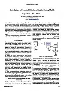
K.K. KAANODIYA, M. RIZWANULLAH strategies. Operational models, such as Pyke (1990) and Caggiano et al. (2006a), consider dynamic deployment of inventories, allocation rules, job prioritization, and other realtime decisions. 1.2 Supply Chain Management System: Supply Chain Management is the logistics of managing the pipe line of goods from contracts with suppliers and receipt of incoming material, control of work-in-process, and finished goods inventories in the plant, to contracting the movement of finished goods through the channels of distribution. It is a network of facilities and distribution options that performs the function of procurement of materials, transformation of these materials into intermediate and finished products, and the distribution of these products to the customers. It exists in both service and manufacturing organizations; although the complexity of the chain may vary greatly form industry to industry. The supply chain management is concerned with the flow of products and information between the supply chain members that encompasses all of those organizations such as suppliers, producers, service providers and customers (See Figure). These organizations linked together to acquire, purchase, convert/manufacture, assemble, and distribute goods and services, from suppliers to the ultimate and users.

Figure-2: Supply Chain Network Section - II SOLUTION METHODOLOGIES: 2.1: The Mean Demand Heuristic Model:

84

MULTI-CRITERIA DECISION MAKING IN DYNAMIC MULTILEVEL DISTRIBUTION SYSTEM

Role of Heuristic Method: Heuristics have become more important in recent years, particularly in the MCDM literature. Many real-world problems are so complex that one cannot reasonably expect to find an exact optimal solution. One broad field involved with such problems is multiple objective combinatorial optimizations, which attempts to address multiple criteria knapsack, traveling salesman, and scheduling problems. Exact solution methods are augmented by simulated annealing, tabu search, and local search techniques. The interested reader is referred to the growing literature on this subject as illustrated by Ulungu and Teghem (1994), Ehrgott and Gandibleux (2000), Jaszkiewicz (2001), and Sun (2003). The rapidly-growing area of evolutionary procedures is related to the role of heuristics in multi-criteria supply chain management system. The Mean Demand Heuristic (MDH) is a problem-specific heuristic that provides us with a good starting point dynamic decision problems. The heuristic can be explained as follows. Let T denote the average cycle time, i.e., the time required to go around the route once and return to the retailer. Let di denote the average demand per customer at the ith retailer. Then, the optimal quantity Qi for the ith retailer, according to this heuristic, is given by Qi = Tdii , where i denotes the mean rate of arrival of customers at the ith retailer. 2.2: Multi-Criteria dynamic decision making (MCDDM) In general, the aim of Multi-criteria or Multi-attribute decision making problems is to find the best compromise solution from all feasible alternatives assessed by predefined criteria (or attributes). This type of problems is widespread in real life situations. There are many methods and approaches proposed in the literature to deal with this static decision process, from utility methods to scoring and ranking ones. However, when facing multi-criteria dynamic multi-level decisions making problems (MCDMLDM), where feedback from step to step is required, there are few contributions in the literature. Usually, a multi-criteria decision model includes main tasks, rating the alternatives by aggregating their classifications for each criterion and then ranking them. In this work we discuss a dynamic multi-criteria decision model because we are addressing decision

85

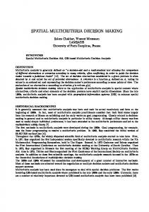
K.K. KAANODIYA, M. RIZWANULLAH paradigms with several iterations, which need to take into account past/historic information, to reach a decision (or consensus). According to Richardson and Pugh system dynamics problems have two main features: “they are dynamic: they involve quantities which change over time”; “involves the notion of feedback.” The main objective of this work is to present some contributions for building general multi-criteria dynamic multi-level decision making (MCDMLDM) models. We will focus on two important aspects of any dynamic spatial-temporal decision problem: a) how to deal with uncertainty in dynamically changing input data; b) and how to consider different criteria importance, depending on criteria satisfaction and on the decision process phase (iteration). These two aspects belong to the classical process of evaluating alternatives of MCDM. General multi-criteria dynamic decision making (MCDDM) architecture is shown in figure 2.

Figure: 3 Rn represents he set of alternatives rating values from iteration n and Hn-1 represents the historic set of rated alternatives from the previous iteration. The feedback is the set of ranked alternatives of iteration n (updated historic set of each iteration). 2.2.1: A MCDM WITH DYNAMIC WEIGHTS OF CRITERIA: Table-1 represents a common MCDM model as a decision matrix. Where Ai, i=1…n represents the ith alternative for decision making, Cj, j=1…m is the weight of the jth

86

MULTI-CRITERIA DECISION MAKING IN DYNAMIC MULTILEVEL DISTRIBUTION SYSTEM criterion and aij is the decision value of the ith alternative corresponding to the jth criterion. Table-1

In this model the decision value of the ith alternative is calculated by: n

dAi = ¦ C j aij ,

i = 1,2, ............m

(1)

i =1

where dAi, Cj and aij are crisp and fixed values. In the dynamical model of MCDM introduced in this paper, the dynamics of each criterion Cj(x), as a function of a main factor, x, is considered for decision making. In this way the calculated decision value dAi(x) is a function of the main factor x (time, cost...). n

dAi ( x) = ¦ C j ( x)aij ,

i = 1,2, ............m

i =1

Hence decision functions, instead of decision values, must be compared for decision making.

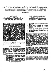
2.2.2: Maximum value of decision function Maximum value of the decision function is potentially a reasonable criteria for decision making between different alternatives. It can be obtained by differentiation the decision function for each alternative

87

(2)

K.K. KAANODIYA, M. RIZWANULLAH

d [dAi ( x)] dx

XMDF i

= 0 Ÿ MDFi = dA i (XMDFi )

(2)

Where XMDFi is the maximum point and MDFi is the maximum value of decision function for the ith alternative. Figure-4 shows the maximum point and the maximum values of the typical decision function dAi.

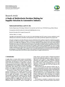
Figure-4: 2.2.3: LINGO Based Multi-criteria Dynamic Multilevel Distribution Model: In this model, we minimize shipping costs over a three tiered distribution system consisting of plants, distribution centers, and customers. Plants produce multiple products, which are shipped to distribution centers. If a distribution center is used, it incurs a fixed cost. Customers are supplied by a single distribution center. This is a three tier (3 stages) shipping/supply chain system. It consists of plants at one level, distribution canters are on second level and customers are on the third level. There are three plants P1, P2 and P3. each plant produced two types of products say A, B; which supplied to 4 distribution canters DC1, DC2, DC3, DC4. Each Distribution centre has fixed cost F. On the third tier system, there five customers say C1, C2, C3, C4 and C5 and the demand for each customer is denoted by D. S indicate the capacity for a product at a plant, but the condition is that each customer Ci (i = 1,2, …..5) is served by one distribution centre which is indicated by Y. X = Quantity to be supplied in tons, and C = Cost/tone of a product from plant to a distribution centre and G = Cost/ton of a product from a distribution centre to a customer.

88

MULTI-CRITERIA DECISION MAKING IN DYNAMIC MULTILEVEL DISTRIBUTION SYSTEM

Plants (Pi)

Distribution Centre (DCi)

Customers (Ci) 1

1

1 2

2 3 3

4 4

Figure-5: Multi Level Decision Model Distribution System 5

LINGO Programming: SETS: ! Two products; PRODUCT/ A, B/; ! Three plants; PLANT/ P1, P2, P3/; ! Each DC has an associated fixed cost, F, and an "open" indicator, Z.; DISTCTR/ DC1, DC2, DC3, DC4/: F, Z;

89

K.K. KAANODIYA, M. RIZWANULLAH ! Five customers; CUSTOMER/ C1, C2, C3, C4, C5/; ! D = Demand for a product by a customer.; DEMLINK( PRODUCT, CUSTOMER): D; ! S = Capacity for a product at a plant.; SUPLINK( PRODUCT, PLANT): S; ! Each customer is served by one DC, indicated by Y.; YLINK( DISTCTR, CUSTOMER): Y; ! C= Cost/ton of a product from a plant to a DC, X= tons shipped.; CLINK( PRODUCT, PLANT, DISTCTR): C, X; ! G= Cost/ton of a product from a DC to a customer.; GLINK( PRODUCT, DISTCTR, CUSTOMER): G; ENDSETS DATA: ! Plant Capacities; S = 80, 40, 75, 20, 60, 75; ! Shipping costs, plant to DC; C = 1, 3, 3, 5, ! Product A; 4, 4.5, 1.5, 3.8, 2, 3.3, 2.2, 3.2, 1, 2, 2, 5, ! Product B; 4, 4.6, 1.3, 3.5, 1.8, 3, 2, 3.5; ! DC fixed costs; F = 100, 150, 160, 139; ! Shipping costs, DC to customer; G = 5, 5, 3, 2, 4, ! Product A; 5.1, 4.9, 3.3, 2.5, 2.7, 3.5, 2, 1.9, 4, 4.3, 1, 1.8, 4.9, 4.8, 2, 5, 4.9, 3.3, 2.5, 4.1, ! Product B; 5, 4.8, 3, 2.2, 2.5, 3.2, 2, 1.7, 3.5, 4, 1.5, 2, 5, 5, 2.3; ! Customer Demands; D = 25, 30, 50, 15, 35, 25, 8, 0, 30, 30; ENDDATA !--------------------------------------------------; ! Objective function minimizes costs.; [OBJ] MIN = SHIPDC + SHIPCUST + FXCOST; SHIPDC = @SUM( CLINK: C * X); SHIPCUST = @SUM( GLINK( I, K, L): G( I, K, L) * D( I, L) * Y( K, L)); FXCOST = @SUM( DISTCTR: F * Z); ! Supply Constraints; \ @FOR( PRODUCT( I):

90

MULTI-CRITERIA DECISION MAKING IN DYNAMIC MULTILEVEL DISTRIBUTION SYSTEM @FOR( PLANT( J): @SUM( DISTCTR( K): X( I, J, K))