Multi-Label Classification with Cutset Networks - JMLR Workshop and ...

JMLR: Workshop and Conference Proceedings vol 52, 147-158, 2016

PGM 2016

Multi-Label Classification with Cutset Networks Nicola Di Mauro Antonio Vergari Floriana Esposito

NICOLA . DIMAURO @ UNIBA . IT ANTONIO . VERGARI @ UNIBA . IT FLORIANA . ESPOSITO @ UNIBA . IT

Department of Computer Science, University of Bari 70125 Bari (Italy)

Abstract In this work, we tackle the problem of Multi-Label Classification (MLC) by using Cutset Networks (CNets), weighted probabilistic model trees, recently proposed as tractable probabilistic models for discrete distributions. We employ CNets to perform Most Probable Explanation (MPE) inference exactly and efficiently and we improve a state-of-the-art structure learning algorithm for CNets by explicitly taking advantage of label dependencies. We achieve this by forcing the tree inner nodes to represent only feature variables and by exploiting structural heuristics while learning the leaf models. A thorough experimental evaluation on ten real-world datasets shows how the proposed approach improves several metrics for MLC, proving it to be competitive with problem transformation methods like classifier chains. Keywords: Multi-label classification; tractable inference; structure learning; cutset networks.

1. Introduction Many real world classification problems involve multiple label classes. The problem of Multi-Label Classification (MLC) concerns learning a mapping from an example to a set of relevant labels. This issue has recently attracted significant attention due to an increasing number of applications, such as image and video annotation, functional genomics in bioinformatics, text categorization, and others (Madjarov et al., 2012). A common approach to MLC is to adopt a problem transformation technique, where a multi-label problem is transformed into one or more single-label problems. A popular problem transformation method to deal with MLC is binary relevance (BR) (Boutell et al., 2004; Tsoumakas et al., 2010). A BR classifier decomposes the MLC problem into a set of single label classification problems, one for each different label. The classifiers are learned independently, thus possibly losing the dependencies among the label variables. However, it is very well known that exploiting these dependencies can significantly improve the classification performance in a MLC scenario, as reported by Dembczy´nski et al. (2012). In order to exploit potential label correlations, the classifier chain approach (CC) (Read et al., 2009) transforms a MLC problem into a chain of binary classification problems, where subsequent binary classifiers in the chain are built upon the predictions of preceding ones. Probabilistic Graphical Models (PGMs) (Koller and Friedman, 2009), such as Bayesian Networks (BNs) and Markov Networks, provide a powerful formalism to model and reason about MLC problems. Indeed, they are able to capture the conditional independence assumptions among random variables into a graph-based representation. Exploiting inference tools in PGMs results in answering different query types such as conditional probability queries and Most Probable Explanation (MPE) queries. Indeed, exploiting MPE inference is one of the approaches to solve MLC (Antonucci et al., 2013; Corani et al., 2014). Nevertheless, learning and inference with PGMs can be challenging. 147

D I M AURO , V ERGARI , AND E SPOSITO

In works like (Waal and Gaag, 2007; Rodr´ıguez and Lozano, 2008; Bielza et al., 2011) the concept of multi-dimensional Bayesian network classifiers (MBCs) for MLC has been introduced. The structure of this kind of networks is learned by partitioning the arcs of the graphs into three sets: links among the label variables (label graph), links among features (features graph) and links between label and features variables (bridge graph). Each subgraph is separately learned and different families of MBCs could be derived by imposing restrictions on the graphical structure of the label and feature subgraphs, e.g. empty graphs, trees, polytrees, and so on. In (Antonucci et al., 2013), an ensemble of BN classifiers has been used for MLC, thus extending to the multi-label case the idea of averaging over a constrained family of classifiers. The label subgraph is assumed to be a tree, and a different classifier for each label is instantiated. Independence of the features given the labels is assumed, thus generalizing to the multi-label case the na¨ıve Bayes assumption. Thanks to this assumption, the optimal bridge subgraph, linking labels and features, can be identified in polynomial time. Due to the high complexity of the inference regarding the MPE joint configuration of all the labels, the same authors switched from the ensemble approach to the single model approach (Corani et al., 2014). To compensate the losing in accuracy of a single model when compared to an ensemble of models, they introduced a more sophisticated structural learning procedure for the label subgraph. Still, the bottleneck remains the high complexity of the inference task during learning and classification. The need for exact and efficient inference procedures has lead to the introduction of Tractable Probabilistic Models (TPMs). An instance of TPMs, tractable PGMs usually trade off expressiveness in exchange for a tractable inference guarantee, see for instance the mixture of tree distributions (Meil˘a and Jordan, 2000). TPMs include, among the others, the recently introduced SumProduct Networks (SPNs) (Poon and Domingos, 2011) as deep architectures encoding probability distributions by layering hidden variables as mixtures of independent components. The greater expressive capacity of SPNs poses new challenges: learning the structure of SPNs involves balancing inference times, hence the whole learning time, and the model accuracy in the terms of a likelihood score (Vergari et al., 2015). To cope with similar issues, Cutset Networks (CNets) have been recently proposed as easy-to-learn TPMs (Rahman et al., 2014). CNets are weighted probabilistic model trees in the form of OR-trees having tree-structured probabilistic models as leaves, and positive weights on inner edges. Inner nodes, i.e., conditioning OR nodes, are associated to random variables and outgoing branches represent conditioning on the values for those variables domains. Structure learning algorithmic variants for CNets have been proven to be both accurate and scalable, given the decomposability property guaranteed by the tree structure (Di Mauro et al., 2015b,a). In this work we show how to employ CNets for MLC problems. As we will show, CNets, differently from MBCs, offer exact and tractable MPE inference, thus alleviating a major issue for MLC. Additionally, we propose a CNet structure learning algorithmic variant for MLC. We modify the searching procedure proposed in (Di Mauro et al., 2015b) by focusing on label dependencies, as it has been proven to be advantageous for MLC (Dembczy´nski et al., 2012). First we force each tree inner node to condition on feature variables only. Then, we apply some heuristics while learning the leaf tree models to put more prominence on the links among label variables while seeking for independence among feature variables. In this way a model can exploit more feature contributions while making predictions about the label variables. We focus on learning a single model and then we prove it to be very competitive against more sophisticated approaches like BR and CC. In a thorough empirical comparison on 10 real-world benchmark datasets, we show our model effectiveness under commonly used metrics for MLC, like accuracy, hamming and exact match scores. 148

M ULTI -L ABEL C LASSIFICATION WITH C UTSET N ETWORKS

2. Cutset Networks In order to introduce the basics about CNets, and before switching to the multi-label case in Section 3, now we assume D to be a set of N i.i.d. instances over the discrete variables X = i {X1 , . . . , Xm }, whose domains are the sets Val(Xi ) = {xji }kj=1 , i = 1, . . . , m. 2.1 Tree-structured probabilistic graphical models A directed tree-structured model (Meil˘a and Jordan, 2000) is a BN in which each variable has at most one parent. The joint probability distribution Q over a set of discrete variables X represented by such a model can be factorized as P (X) = m i=1 P (Xi |Pai ), where Pai stands for the parent variable of Xi , if present. It follows immediately that inference for complete or marginal queries has complexity linear in the number of variables, hence the tractability of tree-structured models. The classic algorithm for learning tree-structured models is that presented in (Chow and Liu, 1968). There it is shown that maximizing the Mutual Information (MI) among random variables in X leads to the best tree, in an information-theoretic sense, approximating the underlying probability distribution of D in terms of the Kullback-Leibler divergence. The learning process for obtaining a tree-structured probabilistic model (CLtree in the following) proceeds as follows. Firstly, for each pair of variables in X, their MI is estimated from D; then a maximum spanning tree is built on the weighted graph induced by the MI as an adjacency matrix. Rooting the tree in a randomly chosen variable and traversing it leads to the learned tree-structured BN. 2.2 Structure and Parameter Learning of Cutset Networks As introduced in (Rahman et al., 2014) and then extended in (Di Mauro et al., 2015b,a), CNets are a hybrid of rooted OR trees and CLtrees, with OR nodes as internal nodes and CLtrees as leaves (see Figure 1). More formally, a CNet is a pair hG, γi, where G = O ∪ {T1 , . . . , TL } is the graphical structure, composed by a rooted OR tree, O, and by leaf trees Tl ; and γ = w ∪ {θ 1 , . . . , θ L } is the parameter set containing the OR tree weights w and the leaf tree parameters θ l . The scope of a CNet G (resp. a leaf tree Tl ), denoted as scope(G) (resp. scope(Tl )), is the set of random variables that appear in it. Each node in the OR tree is labeled by a variable Xi , and each edge emanating from it represents the conditioning of Xi by a value xji ∈ V al(Xi ), weighted by the conditional probability wi,j of conditioning the variable Xi to the value xji . A CNet can be thought of a model tree associating to each instance a weighted probabilistic leaf model. In (Di Mauro et al., 2015b) a recursive definition of CNets has been proposed along with the proof of the decomposability of their log-likelihood and Bayesian Information Criterion (BIC) (Friedman et al., 1997) scores. This lead to a principled algorithm, dCSN, to learn the structure of CNets. A CNet is defined as follows: a) a CLtree, with scope X, is a CNet; b) given Xi ∈ X a variable with |V al(Xi )| = k, graphically conditioned in an OR node, a weighted disjunction of k CNets Gi with same scope X\i is a CNet, where all weights wi,j , j = 1, . . . , k, sum up to one, and X\i denotes the set X minus the variable Xi . Following this definition, the computation of the log-likelihood of a CNet can be decomposed as follows (Di Mauro et al., 2015b). Given a CNet hG, γi over variables X and a set of instances D, its log-likelihood `D (hG, γi) can be computed as: (P Pm if G = {T } ξ∈D i=1 log P (ξ[Xi ]|ξ[Pai ]) `D (hG, γi) = Pk j=1 Mj log wi,j + `Dj (hGj , γ Gj i) otherwise, 149

D I M AURO , V ERGARI , AND E SPOSITO

where the first equation refers to the case of a CNet composed by a single CLtree (ξ[Xi ] is the value assumed by an instance ξ in correspondence of a particular variable Xi ), while the second one specifies the case of an OR tree rooted on the variable Xi , with |V al(Xi )| = k, where, for each j = 1, . . . , k, Gj is the CNet involved in the disjunction with parameters γ Gj , Dj = {ξ ∈ D : ξ[Xi ] = xji } is the slice of D after conditioning on Xi , and Mj = |Dj | its cardinality. `Dj (hGj , γ Gj i) denotes the log-likelihood of the sub-CNet Gj on Dj . By exploiting the log-likelihood decomposition, in dCSN a CNet is grown top-down allowing further expansion, i.e., substituting a CLtree with an OR node only if it improves the log-likelihood. In detail, dCSN starts with a single CLtree, for variables X, learned from D and it checks whether there is a decomposition, i.e., an OR node applied on as many CLtrees as the values of the best variable Xi , providing a better log-likelihood than that scored by the initial tree. If a such decomposition exists, than the decomposition process is recursively applied to the sub-slices Di , testing each leaf for a possible substitution. In order to penalize complex structures and thus avoiding overfitting, a BIC score has been adopted. The BIC score of a CNet hG, γi on data D is defined as: scoreBIC (hG, γi) = log PD (hG, γi) −

log N Dim(G), 2

where Dim(G) is the model dimension, set to the number of OR nodes appearing in G, and N is the size of the dataset D. A Bayesian approach to learn a CLtrees T with parameters θ from data D has been adopted, by exploiting as scoring function P (θ|D) ≈ P (D|θ)P (θ). Considering Dirichlet priors, the regularized model parameter estimates are: θxi |Pai ≈ EP (θx |Pa i

|D,T ) [θxi |Pai ] i

=

Mxi ,Pai + αxi |Pai , MPai + αPai

where Mz is the number of entries in a dataset Dz having the set of variables Z instatiated to z. dCSN, whose source code is public available1 , has been extended to the MLC scenario as described in the next section.

3. Restricted CNets for MLC In this section we will explain how to exploit CNets for MLC. In the following we assume to have a set of training data D of N instances, D = {(xi , yi )}N i=1 . Each training instance has a component xi ∈ X as a vector of M feature values xi = [xi1 , . . . , xiM ], where each xik ∈ R. The set L = {y1 , . . . , yL } denotes the output domain of possible labels. Each vector of attribute values xi for each instance is associated to a subset Yi ⊆ L of these labels, represented by an vector of L binary values yi = [y1i , . . . , yLi ], where yji = 1, if the label yj is assigned to (i.e., is relevant for) the instance, and yji = 0 otherwise (i.e., yji represents the binary relevance of the jth label associated to the ith instance). We assume the instances to be i.i.d. according to a probability distribution ˆ , we P (X, Y) on X × Y. We are interested to learn a model h, s.t., given a test attribute instance x can compute a prediction: ˆ = [ˆ y y1 , . . . , yˆL ] = h(ˆ x) = argmax P (ˆ x, y). y∈{0,1}L

1. https://github.com/nicoladimauro/dcsn

150

M ULTI -L ABEL C LASSIFICATION WITH C UTSET N ETWORKS

X1 0.54

0.46

X2 0.53

X3 0.47

0.13

0.87

Y2

Y1

Y2

Y1

Y2

Y1

Y2

Y1

X3

Y4

Y3

X3

X2

Y4

X2

Y4

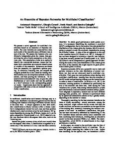
Figure 1: Example of a binary CNet model. Internal nodes on variables Xi are OR nodes, while leaf nodes are CLtrees encoding a direct graphical model.

First we will describe how to perform exact MPE inference by the means of CNets, then we will introduce how we adapt the structure learning algorithm proposed in (Di Mauro et al., 2015b) for MLC. Computing the MPE assignment for the Y is a common way for probabilistic classifiers to tackle the MLC problem (Dembczy´nski et al., 2012). This equals to solve: ˆ = argmax P (y|x) = argmax P (y, x). y y∈{0,1}L

y∈{0,1}L

where the X = x are assumed to be observed as evidence. As already stated, CNets and their leaf tree structures favor tractable probabilistic inference for complete evidences. Here we show how even MPE queries can be answered in time linear to the size of a CNet. In order to do so, one can compute the MPE state for each leaf node and then continue visiting all the OR nodes up to the root, obtaining a complete assignment. For the leaf nodes the MPE state associated to their scope and its corresponding probability can be computed by employing the max-out variant of the Variable Elimination Algorithm, which is guaranteed to be linear in the size of the trees (Koller and Friedman, 2009). For each OR node, defined on the variable Zi , and with outgoing weights w1 , . . . , wk , one would have k possible MPE states, s1 , . . . , sk , corresponding to each sub-tree. Each state, alongside its MPE probability pi , i = 1, . . . , k, has been computed when exploring the child nodes. If Zi appears as evidence, i.e. Zi ∈ X, then one simply chooses the child branch corresponding to its value. Otherwise, the branch j ∗ = argmaxj=1,...,k wj pj and the corresponding MPE state are chosen. This is also linear in the number of child sub-trees. 3.1 Restricted Structure Learning Probabilistic multi-label classifiers can be learned by optimizing one particular loss function, e.g. subset 0/1 loss or hamming loss. While doing this, they may try to elicit the marginal (resp. conditional) label dependencies if they focus on modeling p(Y) (resp. p(Y|X)) (Dembczy´nski et al., 2012). Our approach consists in learning a CNet while optimizing the joint likelihood, but guiding 151

D I M AURO , V ERGARI , AND E SPOSITO

the structure learning algorithm to focus on the label dependence relationships. We employ several heuristics to achieve this, both during the CNet structure growing phase and the leaf tree learning steps. The common idea behind all of them is to prefer modeling more accurately the dependencies among the Y than the ones over the X. First, we limit the OR split tests to be taken on the X variables only while growing a CNet. This leads to particular networks which we call Restricted CNets (RCNets). By doing this we force the Y to be strictly dependent from the X appearing in the internal nodes. This is pretty evident when using an RCNet as a generative model. This also helps the Chow-Liu algorithm to better focus on the Y variable interactions. The CNet in Figure 1 is an RCNet as well, since label variables are represented only in the leaves: e.g., the leftmost leaf models the interactions among all label variables but on the subset of the dataset where X1 and X2 variables are set to 0. A second constraint has been imposed on the structure of the BNs in the leaves: each label variable and each feature variable can only have as a parent a label variable. This implies that features variables shall be independent given the label variables. From the perspective of a MBC, this constraint translates into the label subgraph to be a tree, and the feature sub-graph to be empty. However, differently from a single MBC, in an RCNet we have several possible variations of such templated trees, one for each leaf and modeling different dependencies for different views of the data. In this way we force to model the dependencies among the class variables, and giving the feature to independently contribute in the MPE inference evaluation. In order to fulfill this constraint, the classical Chow-Liu tree algorithm described in Section 2 has been modified as reported in Algorithm 1 leading to restricted tree-structured PGMs. After having computed the mutual information matrix MI between all the variables, we forcibly alter some of its values. Let the MI matrix be represented as a block matrix:   MIX,X MIX,Y MI = MITX,Y MIY,Y where MIX,X (resp. MIY,Y ) denotes the sub-matrix comprising the mutual information values among variables in X (resp. Y) and MIX,Y denotes the sub-matrix comprising the values among one feature and one label variables. We first set MIX,X = 0 to enforce the label conditional independence of the X, then we boost the mutual information values for the label variables by setting MIY,Y = MIY,Y + max(MI), thus forcing the insertion of all the edges over the Y in the spanning tree before considering the interactions with the X.

4. Experimental Evaluation In this section we present the experimental setup to detail the performance evaluation metrics, the multi-label datasets, the algorithms and their experimental settings. The source code of our algorithm, scripts and datasets are made publicly available2 . 4.1 Evaluation Metrics Recall that given a multi-label dataset consisting of N instances, each one associated with a set of labels Yi ⊆ L, denoted by a vector of L binary values yi , a classifier predicts a set of labels ˆ denoted by a vector of L binary values y ˆ i . In MLC there is no one single way to assess the Y, 2. https://github.com/nicoladimauro/dcsn

152

M ULTI -L ABEL C LASSIFICATION WITH C UTSET N ETWORKS

Algorithm 1 LearnRestrictedCLT(D, X, Y) 1: Input: a set of instances D over a set of features X and labels Y 2: Output: hT , θi, a tree T with parameters θ encoding a pdf over X ∪ Y 3: MI ← 0|X∪Y|×|X∪Y| 4: for each Vi , Vj ∈ X ∪ Y do 5: M Iij ← estimateMutualInformation(Vi , Vj , D) 6: 7: 8: 9: 10: 11:

MIX,X ← 0 MIY,Y ← MIY,Y + max(MI) T ← maximumSpanningTree(MI) T ← traverseTree(T ) θ ← computeFactors(D, T ) return hT , θi

. label conditional independence of the Xs . forcing dependencies among the Ys

classifier performance. It is well known in the literature that different metrics focus on different dependency relationships among the label variables, and are better optimized by taking into account those dependencies (Dembczy´nski et al., 2012). We employ three different metrics to assess the overall performance of CNets and the improvement gained by RCNets. We want to prove that even a single CNet can be competitive against more sophisticated models and that the proposed heuristics for RCNets are indeed meaningful for MLC. Namely, the three employed metrics are: N

H AMMING S CORE =

L

1 XX i I(yj = yˆji ), NL i=1 j=1

E XACT M ATCH =

ACCURACY =

1 N 1 N

N X i=1 N X i=1

ˆ i ), I(yi = y ˆ i| |yi ∧ y , ˆ i| |yi ∨ y

where I(C) is the indicator function, while ∧ and ∨ are the bitwise logical AND and OR operations, respectively (Madjarov et al., 2012). The E XACT M ATCH measure, or 0/1 LOSS as a loss measure, computes the percentage of ˆ matches the true set of labels y exactly. On the other side, instances whose predicted set of labels y the H AMMING S CORE rewards methods for predicting individual labels well. While the E XACT M ATCH is a very strict evaluation measure, the H AMMING S CORE tends to be very lenient. Finally, ACCURACY is a label set-based measure defined by the Jaccard similarity coefficients between the predicted and true set of labels. 4.2 Datasets A set of 10 numerical traditional multi-label datasets (accessible from the MULAN3 , MEKA4 , and LABIC5 websites) has been used in the experiments. These datasets belong to a wide variety of ap3. http://mulan.sourceforge.net/. 4. http://meka.sourceforge.net/. 5. http://computer.njnu.edu.cn/Lab/LABIC/LABIC_Software.html.

153

D I M AURO , V ERGARI , AND E SPOSITO

Arts-Yahoo Business-Yahoo CAL500 Emotions Flags Health-Yahoo Human Plant Scene Yeast

Domain Text Text Music Music Images Text Biology Biology Images Biology

M 500 500 68 72 19 500 440 440 294 103

N 7484 11214 502 593 194 9205 3106 978 2407 2417

L 26 30 174 6 7 32 14 12 6 14

LCard 1.653 1.598 26.043 1.868 3.391 1.644 1.185 1.078 1.073 4.237

LDens 0.063 0.053 0.149 0.311 0.484 0.051 0.084 0.089 0.178 0.302

LDist 599 233 502 27 54 335 85 32 15 198

Table 1: Dataset descriptions: number of attributes (M ), instances (N ), and labels (L). plication domains and their labels range from 6 to 174, while the number of attributes ranges from 19 to 500, and the number of examples ranges from 194 to 11214. Table 1 reports the information about the adopted datasets, where M , N and L represent the number of attributes, instances, and possible labels respectively. Furthermore, for each dataset D the following statistics are also reported: Label P PL LCard(S) i Cardinality: LCard(D) = N1 N and Distinct j=1 yj , Label Density: LDens(D) = i=1 L Labels: LDist(D) = |{y|∃(x, y) ∈ D}|. Since our current implementation of CNets works on binary data we discretized all the numeric features for each dataset implementing the Label-Attribute Interdependence Maximization (LAIM) (Cano et al., 2016) discretization method for multi-label data. We run all the algorithms in these experiments on the datasets preprocessed by LAIM. 4.3 Algorithms and setup For the experimental evaluation, we compared both CNet and RCNet implementations, CNET and RCNET6 , to different algorithms. Both CNET (obtained by dropping lines 6-7 in Algorithm 1) and RCNET limit OR nodes on X variables, while in addition RCNET modify the MI matrix in order to fulfill the (in)dependency constraints. Other algorithms have been run using their openly available implementations in MEKA7 (release 1.9.0). First, due to the lack of openly available implementations of BNs structure learning algorithms for MLC, we include in the comparison the Bayesian Chain Classifier (BCC) (Zaragoza et al., 2011), which builds a probabilistic CC after learning the structure of a BN for MLC. As reported in (Zaragoza et al., 2011), BCC is highly competitive against other Bayesian multi-dimensional classifiers such as those reported in (Waal and Gaag, 2007; Bielza et al., 2011). Then, even if they are not directly comparable to CNets, as they are ensembles as problem transformation methods, we included both binary relevance method (BR) and the classifier chains method (CC). As base classifiers we used Na¨ıve Bayes (NB) and Tree Augmented Na¨ıve Bayes (TAN), leading respectively to six different multi-label classifier variants: BRNB, CCNB, BRTAN and CCTAN. Parameters were set as suggested by the MEKA software8 . 6. Both have be run with -d 0.6, leaving all the other parameters set to default value. 7. Available at http://meka.sourceforge.net. 8. TAN with SimpleEstimator with alpha=1, and scoreType = BAYES. BCC with NaiveBayes as classifier and a default value for dependencyType. All the scripts for reproduce the MEKA results reported in this paper are available at https://github.com/nicoladimauro/dcsn. All experiments have been run on a 4-core Intel Xeon E312xx (Sandy Bridge) @2.0 GHz with 8Gb of RAM and Linux kernel 3.13.0-39.

154

M ULTI -L ABEL C LASSIFICATION WITH C UTSET N ETWORKS

Dataset Arts Business CAL500 Emotions Flags Health Human Plant Scene Yeast Avrg rank

RCNET 0.432 (6) 0.728 (1) 0.203 (3) 0.554 (2) 0.563 (2) 0.603 (3) 0.361 (1) 0.397 (1) 0.669 (1) 0.464 (2) 1.7

CCTAN 0.372 (4) 0.703 (4) 0.188 (5) 0.563 (1) 0.565 (1) 0.611 (1) 0.301 (3) 0.313 (3) 0.658 (2) 0.452 (3) 2.8

BRTAN 0.391 (3) 0.704 (3) 0.251 (2) 0.542 (5) 0.544 (4) 0.610 (2) 0.249 (5) 0.308 (4) 0.634 (3) 0.479 (1) 3.2

CNET 0.399 (2) 0.719 (2) 0.187 (5) 0.499 (6) 0.526 (6) 0.587 (4) 0.306 (2) 0.354 (2) 0.530 (4) 0.442 (4) 3.7

CCNB 0.376 (4) 0.68 (6) 0.184 (7) 0.553 (3) 0.542 (5) 0.578 (6) 0.258 (4) 0.298 (5) 0.530 (4) 0.404 (7) 5.1

BRNB 0.358 (7) 0.660 (7) 0.252 (1) 0.512 (6) 0.545 (3) 0.582 (5) 0.197 (7) 0.278 (7) 0.528 (6) 0.429 (5) 5.4

BCC 0.331 (5) 0.658 (5) 0.287 (4) 0.475 (4) 0.550 (6) 0.521 (6) 0.265 (6) 0.229 (6) 0.563 (7) 0.453 (6) 5.6

Table 2: The performance of the multi-label learning approaches in terms of the ACCURACY measure. In parenthesis the rank of the algorithm for a given dataset.

Dataset Arts Business CAL500 Emotions Flags Health Human Plant Scene Yeast Avrg rank

RCNET 0.937 (2) 0.973 (1) 0.854 (1) 0.783 (4) 0.709 (4) 0.965 (1) 0.894 (1) 0.892 (3) 0.879 (3) 0.773 (1) 2.2

BRTAN 0.931 (3) 0.965 (2) 0.814 (4) 0.797 (1) 0.710 (3) 0.963 (3) 0.890 (2) 0.894 (2) 0.898 (1) 0.765 (2) 2.8

CCTAN 0.940 (1) 0.965 (2) 0.823 (3) 0.786 (3) 0.709 (4) 0.964 (2) 0.870 (4) 0.901 (1) 0.888 (2) 0.749 (3) 2.9

CNET 0.937 (2) 0.974 (1) 0.854 (1) 0.737 (6) 0.680 (6) 0.964 (2) 0.894 (1) 0.888 (5) 0.838 (5) 0.765 (2) 3.1

BRNB 0.926 (4) 0.957 (4) 0.813 (5) 0.787 (2) 0.723 (1) 0.959 (4) 0.884 (3) 0.890 (4) 0.874 (4) 0.732 (4) 4.1

BCC 0.936 (5) 0.969 (5) 0.833 (2) 0.760 (6) 0.716 (2) 0.956 (5) 0.891 (6) 0.862 (5) 0.867 (6) 0.754 (5) 5.5

CCNB 0.923 (6) 0.942 (6) 0.684 (6) 0.768 (5) 0.708 (6) 0.955 (6) 0.827 (5) 0.884 (5) 0.816 (5) 0.720 (6) 6.4

Table 3: The performance of the multi-label learning approaches in terms of the H AMMING SCORE measure. In parenthesis the rank of the algorithm for a given dataset. .

4.4 Results and discussion The results for each evaluation metric and for each classification algorithm on all the datasets are reported in Table 2, 3 and 4. RCNET outperforms the other methods in 10 (CCNB), 9 (BRNB and BCC), and 7 (CCTAN and BRTAN) cases in terms of the ACCURACY measure (Table 2). In terms of the H AMMING S CORE measure, RCNET is superior to the others in 10 (CCNB and BCC), 8 (BRNB), 6 (BRTAN) and 5 (CCTAN) cases (Table 3). Regarding the E XACT M ATCH measure, RCNET is ranked better in 9 (BRNB, CCNB and BCC), 8 (BRTAN), 6 (CCTAN) cases (Table 4). By looking at the average ranks, even CNET consistently outperforms BCC, BRNB and CCNB for all the three measures. We can see from these results that even if RCNET learns a single model, it is competitive to other approaches. It performs better that other methods in terms of the ACCURACY and E XACT M ATCH measure. 155

D I M AURO , V ERGARI , AND E SPOSITO

Dataset Arts Business CAL500 Emotions Flags Health Human Plant Scene Yeast Avrg rank

RCNET 0.313 (1) 0.567 (1) 0.000 (1) 0.295 (1) 0.170 (2) 0.456 (2) 0.263 (1) 0.344 (1) 0.554 (1) 0.147 (2) 1.4

CCTAN 0.275 (2) 0.548 (2) 0.000 (1) 0.282 (3) 0.212 (1) 0.478 (1) 0.139 (3) 0.247 (2) 0.498 (3) 0.169 (1) 2.3

CNET 0.302 (1) 0.565 (1) 0.000 (1) 0.260 (1) 0.185 (1) 0.448 (1) 0.260 (1) 0.333 (1) 0.492 (1) 0.129 (1) 2.7

BRTAN 0.247 (4) 0.545 (3) 0.000 (1) 0.295 (1) 0.108 (6) 0.437 (3) 0.141 (2) 0.207 (3) 0.518 (2) 0.120 (3) 3.5

CCNB 0.251 (3) 0.520 (5) 0.000 (1) 0.265 (5) 0.129 (3) 0.407 (6) 0.085 (5) 0.185 (4) 0.248 (5) 0.117 (4) 4.9

BRNB 0.234 (6) 0.518 (6) 0.000 (1) 0.280 (4) 0.114 (5) 0.425 (4) 0.100 (4) 0.181 (5) 0.375 (4) 0.101 (5) 5.2

BCC 0.187 (5) 0.410 (4) 0.000 (1) 0.207 (6) 0.109 (3) 0.247 (5) 0.150 (6) 0.110 (6) 0.422 (6) 0.074 (6) 5.6

Table 4: The performance of the multi-label learning approaches in terms of the E XACT M ATCH measure. In parenthesis the rank of the algorithm for a given dataset. .

1 2 3 4 5 6 7

1 2 3 4 5 6 7

1 2 3 4 5 6 7

RCNET CCTAN BRTAN CNET

CD = 2.8483

CD = 2.8483

CD = 2.8483

BCC BRNB CCNB

RCNET BRTAN CCTAN CNET

CCNB BCC BRNB

RCNET CCTAN CNET BRTAN

BCC BRNB CCNB

Figure 2: The critical diagrams for the ACCURACY (left), H AMMING S CORE (center) and E XACT MATCH (right) evaluation measures: results from the Nemenyi post-hoc test at p=0.05 significance level.

In order to assess whether the overall differences in performance are statistically significant a post-hoc Nemenyi test (Demˇsar, 2006) has been conducted comparing all the classifiers to each others. With a Nemenyi test the performances of two classifiers are significantly different if their average ranks differ by more than some critical distance (CD), obtained by taking into account the number of algorithms, the number of datasets and a critical value for a given significance level p. Figure 2 reports the results from the Nemenyi post-hoc test with average rank diagrams, where the average ranks of the algorithms are drawn on an enumerated axis. The best ranking algorithms are at the left-most side of the diagram, and the horizontal bold lines connect the vertical lines for the average ranks of the algorithms that do not differ significantly. As we can see, the differences are not statistically different at p = 0.05 significance level when compared to those obtained by the methods BRTAN and CCTAN. However, note that RCNETs are single models and as such they could be incorporated into sophisticated problem transformation schemes as CC and BR. Devising a way to blend CNet structure learning into these schemes is an interesting future line of work. 156

M ULTI -L ABEL C LASSIFICATION WITH C UTSET N ETWORKS

5. Conclusions In this paper, we tackled the MLC problem by employing CNets, a recently proposed tractable probabilistic model for representing multi-dimensional discrete distributions. We exploited CNets to efficiently and exactly solve an MPE formulation of MLC. We devised a structure learning algorithmic variant to cope with the prominence of label dependencies, a crucial issue in MLC. The experimental evaluation on 10 real-world datasets showed how our approach can effectively improve the accuracy, exact and hamming scores, proving itself to be highly competitive against more complex ensemble approaches.

Acknowledgments Work partially supported by the European Commission through the project MAESTRA - Learning from Massive, Incompletely annotated, and Structured Data (Grant number ICT-2013-612944), and by the project PUGLIA@SERVICE (PON02 00563 3489339) financed by the Italian Ministry of University and Research (MIUR). Experiments executed on the resources made available by two projects financed by the MIUR: ReCaS (PONa3 00052) and PRISMA (PON04 a2A).

References A. Antonucci, G. Corani, D. D. Mau´a, and S. Gabaglio. An ensemble of bayesian networks for multilabel classification. In Proceedings of IJCAI, pages 1220–1225, 2013. C. Bielza, G. Li, and P. Larra˜naga. Multi-dimensional classification with bayesian networks. International Journal of Approximate Reasoning, 52(6):705–727, 2011. M. R. Boutell, J. Luo, X. Shen, and C. M. Brown. Learning multi-label scene classification. Pattern Recognition, 37(9):1757–1771, 2004. A. Cano, J. M. Luna, E. L. Gibaja, and S. Ventura. LAIM discretization for multi-label data. Information Sciences, 330:370–384, 2016. C. Chow and C. Liu. Approximating discrete probability distributions with dependence trees. IEEE Transactions on Information Theory, 14(3):462–467, 1968. G. Corani, A. Antonucci, D. D. Mau´a, and S. Gabaglio. Trading off speed and accuracy in multilabel classification. In Proceedings of PGM, pages 145–159. Springer, 2014. K. Dembczy´nski, W. Waegeman, W. Cheng, and E. H¨ullermeier. On label dependence and loss minimization in multi-label classification. Machine Learning, 88(1):5–45, 2012. J. Demˇsar. Statistical comparisons of classifiers over multiple data sets. Journal of Machine Learning Research, 7:1–30, 2006. N. Di Mauro, A. Vergari, and T. M. Basile. Learning bayesian random cutset forests. In Proceedings of ISMIS, pages 122–132. Springer, 2015a. N. Di Mauro, A. Vergari, and F. Esposito. Learning accurate cutset networks by exploiting decomposability. In Proceedings of AIXIA, pages 221–232. Springer, 2015b. 157

D I M AURO , V ERGARI , AND E SPOSITO

N. Friedman, D. Geiger, and M. Goldszmidt. Bayesian network classifiers. Machine learning, 29 (2-3):131–163, 1997. D. Koller and N. Friedman. Probabilistic Graphical Models: Principles and Techniques. MIT Press, 2009. G. Madjarov, D. Kocev, D. Gjorgjevikj, and S. Deroski. An extensive experimental comparison of methods for multi-label learning. Pattern Recognition, 45(9):3084–3104, 2012. M. Meil˘a and M. I. Jordan. Learning with mixtures of trees. Journal of Machine Learning Research, 1:1–48, 2000. H. Poon and P. Domingos. Sum-Product Network: a New Deep Architecture. NIPS 2010 Workshop on Deep Learning and Unsupervised Feature Learning, 2011. T. Rahman, P. Kothalkar, and V. Gogate. Cutset networks: A simple, tractable, and scalable approach for improving the accuracy of Chow-Liu trees. In Machine Learning and Knowledge Discovery in Databases, volume 8725 of LNCS, pages 630–645. Springer, 2014. J. Read, B. Pfahringer, G. Holmes, and E. Frank. Classifier chains for multi-label classification. In Proceedings of the European Conference on Machine Learning and Knowledge Discovery in Databases: Part II, pages 254–269. Springer-Verlag, 2009. J. D. Rodr´ıguez and J. A. Lozano. Multi-objective learning of multi-dimensional Bayesian classifiers. In Proceedings of the Eighth International Conference on Hybrid Intelligent Systems, pages 501–506, 2008. G. Tsoumakas, I. Katakis, and I. P. Vlahavas. Mining multi-label data. In Data Mining and Knowledge Discovery Handbook, 2nd ed., pages 667–685. Springer, 2010. A. Vergari, N. Di Mauro, and F. Esposito. Simplifying, Regularizing and Strengthening SumProduct Network Structure Learning. In ECML-PKDD 2015, 2015. P. R. Waal and L. C. Gaag. Inference and learning in multi-dimensional bayesian network classifiers. In 9th European Conference on Symbolic and Quantitative Approaches to Reasoning with Uncertainty, pages 501–511. Springer, 2007. J. H. Zaragoza, L. E. Sucar, E. F. Morales, C. Bielza, and P. Larra˜naga. Bayesian chain classifiers for multidimensional classification. In Proceedings of the 22nd IJCAI. AAAI Press, 2011.

158