Multi-Objective Evolutionary Algorithm for Land-Use ... - IIT Kanpur

Multi-Objective Evolutionary Algorithm for Land-Use Management Problem Dilip Datta, Kalyanmoy Deb KanGAL, Department of Mechanical Engineering Indian Institute of Technology Kanpur Kanpur - 208 016, India {ddatta,deb}@iitk.ac.in Carlos M. Fonseca, Fernando Lobo, Paulo Condado DEEI, Faculty of Science & Technology, University of Algarve, Campus de Gambelas 8000-117 Faro, Portugal {cmfonsec,flobo,pcondado}@ualg.pt KanGAL Report Number 2006005

Abstract Due to increasing population, and human activities on land to meet various demands, land uses are being continuously changed without a clear and logical planning with any attention to their long term environmental impacts. Thus affecting the natural balance of the environment, in the form of global warming, soil degradation, loss of biodiversity, air and water pollution, and so on. Hence, it has become urgent need to manage land uses scientifically to safeguard the environment from being further destroyed. Owing to the difficulty of deploying field experiments for direct assessment, mechanistic models are needed to be developed for improving the understanding of the overall impact from various land uses. However, very little work has been done so far in this area. Hence, NSGA-II-LUM, a spatial-GIS based multi-objective evolutionary algorithm, has been developed for three objective functions: maximization of economic return, maximization of carbon sequestration and minimization of soil erosion, where the latter two are burning topics to today’s researchers as the remedies to global warming and soil degradation. The success of NSGA-II-LUM has been presented through its application to a Mediterranean landscape from Southern Portugal.

Keywords: Land-use management, multi-objective optimization, evolutionary algorithms, NSGA-II, NSGA-II-LUM.

1

Introduction

Land-use management problem/practice may be defined as the process of allocating different competitive land uses/activities, such as agriculture, forest, industries, recreational activities or conservation, to different units of a landscape to meet the desired objectives 1

of land managers (Stewart et al. [40]). Land uses and their changes from patterns to processes should be determined by land-use management practices. Land-use management practices include many items, like geographic distribution of land, status of land resources and their suitability, land use dynamics, policy interventions, socio-economic practices and compulsions, science and technology inputs, and so on. Thus, various landuse management practices are to be understood in order to develop an integrated land use policy framework for improving soil quality, ensuing biomass production and food security, maintaining environmental stability, and extending socio-economic benefits (Gautam and Raghavswamy [21]). The most important constraint on the progress of human society is soil. The survival of all animals, including humans, depends on plants that grow in soil, and hence, it is very important to maintain the quality of soil. Although humans can improve the properties of soils through their agricultural activities, by far the most common effects of human activities on soils are degradation and destruction, and environmental instability (Huston [24]). One burning example of environmental instability is global warming. Human activities, such as burning of coal and other fossil fuels for energy, and extensive land use changes for agriculture and development by clearing forests or draining wet-lands, are continuously affecting the biosphere, thus altering the natural balance of atmospheric greenhouse gases (GHGs) by increasing the amount of their constituents, particularly CO2 which is the major constituent of GHGs (Bhadwal and Singh [4]; Bongen [6]). As a consequence, the layer of GHGs is becoming thicker and thicker, thus causing global warming by capturing excess solar heat near the Earth’s surface, which otherwise would have been radiated back to the atmosphere (Bongen [6]). However, the atmospheric concentration of CO2 can be lowered through carbon sequestration, i.e., (1) reducing the emissions of carbon through the reduction in the demand of fossil fuels, and other human activities, such as deforestation and land use changes, and (2) increasing the rates of removal of CO2 from the atmosphere through the growth of terrestrial biomass, and storing carbon in terrestrial, oceanic, or freshwater aquatic ecosystems (Bhadwal and Singh [4]; USDA:GCFS [43]). There is major potential for increasing carbon storage in soil through restoration of degraded soils, and widespread adoption of soil conservation practices (USDA:GCFS [43]). Another big issue, associated with land uses, is soil degradation - the visible part of which is soil erosion, where soil particles are transported from one place to another place by gravity, water or wind (Anthoni [2]). Though plants can provide protective cover on land by preventing soil erosion, the loss of protective plants, through deforestation, over-grazing, and ploughing, makes soil vulnerable for being eroded. In addition, over-cultivation and compaction cause soil to lose its structure and cohesion, thus becoming more easily erodible (BCB:UWC [3]). Though many protective measures, to the impacts of improper uses of land and its resources, are already known, those are yet to be used fully due to lack of proper scientific knowledge for their effective implementation. Owing to the difficulty of deploying field experiments for direct assessment, it is important to develop mechanistic models, through extensive study, for improving the understanding of the overall impact from various land uses. However, very limited works have been done so far in this direction. Hence, the present work has been aimed at modeling an optimization tool for allocating suitable land uses to different units of a landscape, which would help in achieving multiple objectives simultaneously. In this regard, NSGA-II-LUM, a spatial-GIS based multi-objective EA, has also been developed to handle the problem. It employs NSGA-II (Deb [13]; Deb et al. [15]), an EA-based multi-objective optimizer, with specially designed representation and EA operators. NSGA-II-LUM has been designed for optimizing three non-commensurable

2

objective functions, subject to a set of physical and ecological constraints. The chosen objectives are maximization of socio-economic benefit, maximization of carbon sequestration, and minimization of soil erosion, where the latter two are burning topics to today’s researchers as the remedies to global warming and soil degradation. Physical constraints on a unit, to make it permissible to hold a land-use in it, have been imposed on geomorphological structure, and ecological constraints on land uses have been imposed to insure spatial coherence of a landscape. The success of NSGA-II-LUM has been presented through its application to a Mediterranean landscape, located in Southern Portugal.

2

Related Works

Bhadwal and Singh [4] made a comparative estimate of land-use and carbon sequestration potential of different forestry options in India. Three different models were generated with different land-use options, where the models estimate the amount of sequestered carbon by approximating land-use and relative biomass changes. Kerr et al. [26] designed the integrated dynamics of land-use system and carbon-pools by combining an ecological model with an economic model. The models are combined so that ecological conditions affect the land-use choices, and vice versa. Liu and Bliss [28] developed a general ecosystem model to dynamically simulate the influences of rainfall-induced soil erosion and deposition on carbon dynamics in soil profiles. According to them, erosion reduces carbon storage at eroding sites, while deposition increases carbon storage at depositional areas, thus balance the global atmospheric carbon budget through their impacts on the net exchange of carbon between terrestrial ecosystems and the atmosphere. In another work, Liu et al. [29] investigated the carbon sequestration of an ecoregion by assimilating historical data on land-use and land-cover changes. In the past, land-use management problem was tackled using linear programming (LP) approaches. However, the recent trends, such as increased involvement of stakeholders, increased complexity on decision making, spatial integrity, and use of Geographical Information Systems (GIS), have made the problem more complicated by transforming it into a pure integer programming (IP) problem (Stewart et al. [40]). As a result, IP approaches were started to use in this problem as the LP approaches suffer from the disadvantages of handling integer variables and spatial coordinates. However, both LP and IP approaches are essentially single objective optimizers, and multiple objectives are required to be combined into a single scalar value (Ducheyne [17]). Then non-classical heuristic approaches, such as simulated annealing, greedy growing algorithms, and tabu search, were also found applicable to this problem. However, though these approaches are robust, fast and capable of solving large combinatorial problems, they do not guarantee the optimal solution. Recently, Genetic/Evolutionary algorithms (GAs/EAs), biological evolution-based heuristic approaches, have been found suitable enough to tackle the problem (Aerts et al. [1]). Unlike other heuristic approaches, GAs/EAs are general-purpose search methods, combining elements of directed and stochastic search, which can make a remarkable balance between exploitation and exploration of a search space (ISDAG [25]). Matthews et al. [30; 32] explored the potential of applying GA to spatially integrated land-use management problem. Matthews et al. [31] developed a GA-based spatial decision support system (DSS) that allows land managers to explore their land use options and potential impacts of land use changes. In another work, Matthews et al. [33] developed a multi-objective GA-based DSS to define the structure of trade-off between two conflicting and non-commensurable objectives of 3

financial and landscape diversity. Stewart et al. [40] used a GA, along with a goal programming/reference point approach, to another spatially integrated problem, involving two objectives: minimization of cumulative cost, and compactness of areas under each land-use. Seixas et al. [38] proposed another EA to study future land-use configuration under two objectives of maximization of carbon sequestration and minimization of soil loss.

3

Land-Use Management as a Multi-Objective Optimization Problem

Land-use management problem involves the allotment of different competitive land uses to different units of a landscape to meet the desired objectives of land managers. This is a complex process, since the decisions must be made not only on achieving the overall objectives of land managers, but also on the selection of an effective land-use for a unit, which is again subject to a number physical and ecological restrictions (Stewart et al. [40]). This clearly leads the problem to an optimization problem, where different objectives of land managers are to be optimized, subject to the restrictions imposed on the selection of an effective land-use for a unit. Based on this, the problem can be defined and formulated as mentioned below:

3.1

Constraints in Land-Use Management Problem

A land-use, effective at one location, may be totally ineffective at another location. Likewise, a land-use that works well in one season, may not work, at all, in another season. For the effective implementation of a land-use, the consequences of spatial and temporal variations in soils and climate must be taken into account. Another constraint is on the choice of land uses which have a major influence on runoff and erosion. Any land-use practices, that reduce runoff, have the benefit of increasing the local water supply and reducing soil loss. However, such practices impose limitations on agricultural and technological input, and sustainable levels of productivity (Huston [24]). On the other hand, water availability imposes strong constraints on technologies for sustainability, and even subtle variations in the distribution of rainfall can have a major impact on the sustainability of various agricultural systems (Ellis and Galvin [19] in Huston [24]). Apart from these, landscape ecology and biodiversity are also major issues which are to be taken into care during any management planning. In case of nature reserves, it is seen that the size of a patch, the amount of edges, and the continuity of patches can affect the ability to support different species (Davis et al. [11] in Ducheyne [17]), for which compact and contiguous patches are always preferred (Diamond [16] in Venema et al. [44]). Based on these, the physical and ecological constraints on the problem can be defined as below (Seixas et al. [38]): • Physical constraints on geomorphological structure: 1. A land-use should be applied in a unit, only if it is permitted in the soil of that unit, 2. The slope of a unit should be within the permitted range of slope for the landuse applied in that unit, 3. The aridity index of a unit should be within the permitted range of aridity index for the land-use applied in that unit, and 4

4. Topographic soil wetness index (TSWI) of a unit should be within the permitted range of TSWI for the land-use applied in that unit. • Ecological constraints on spatial coherence: 1. Patch-Size Constraint: Area in a patch (a set of contiguous units) of a landuse should be within the permitted range of area in a patch for that land-use, and 2. Total Area Constraint: Total area under a land-use in a landscape should be within the permitted range of total area for that land-use.

3.2

Objective Functions in Land-Use Management

Land-use management depends on the proper evaluation of the potential of every unit of a landscape to sustainably support many services that a society needs. Every unit of a landscape has the potential to perform several functions, which might be contributing to agricultural or industrial productivity, maintaining biodiversity, and minimizing runoff. Information on physical and biological properties of a landscape is available from soil surveys, topographic maps, and satellite images. However, using this information effectively requires both scientific understanding and technological infrastructure. Land-use management must be a multidisciplinary effort, using the expertise of hydrologists, economists, ecologists, social scientists, agronomists, foresters, etc. We already know which of the available technologies would likely contribute to the sustainability of a particular sector of human activity. What is still lacking is an understanding of the interactions between various sectors, and how land-use management can simultaneously produce positive results in several sectors. Since sustainability must address multiple objectives of human and natural systems, land-use prioritization must be based on proper evaluations of all the potential uses of each unit of a landscape (Huston [24]). Realizing the urgent needs of a society, the following three objectives have been considered in the present study: 1. Maximization of net present economic return, 2. Maximization of net amount of carbon sequestration, and 3. Minimization of net amount of soil erosion.

3.3

Mathematical Formulation

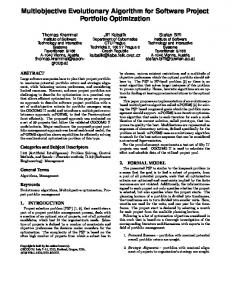
Different segments of a landscape vary from each other on the basis of their geomorphological structures. These differences restrict a land-use to be applied only in particular segment(s) which meet(s) the requirements for that land-use. Therefore, a landscape needs to be considered as composed of a number of units. These units need not to follow any common pattern, but are identified on the basis of their areas, and/or other distinct properties. However, for the ease of mathematical analysis, a landscape can be represented by a two-dimensional grid, as shown in fig.1 by i- and j-axes of the three-dimensional matrix, where each grid represents a unit of the landscape. Then a unit can be identified by its location (i, j) in the landscape. The third axis of the matrix, the t-th axis as shown in fig.1, represents the time-scale of a unit over a planning horizon. Based on this, the land-use management problem, as a multi-objective optimization problem, can now be expressed mathematically as below: 5

e11

e12 e13

e14

e21

e22

e23

e24

e31

e32

e33

e34

e41

e42

e43

e44

n

y

y2

y2

n

y

y1

y1 y 2

n

y1

y1

y1 y2

y

y2

y2

y2

t

yn

yn

n

yn

y

Land use

y1

yn

y1 y 2 y1

Ye ar

Ye ar

i

Land use

j

Figure 1: Model of a landscape. Let,

E Ru Cu U T

Number of events (land uses). Number of rows of units in a landscape. Number of columns of units in the landscape. Total number of units in the landscape (= Ru .Cu ). Total number of years over the planning horizon.

Xe,i,j

= 1, if event e is applied in unit (i, j), = 0, otherwise.

• Objectives functions: 1. Maximize net present economic return f1 ≡

Cu Ru X E X X

Xe,i,j .me,i,j ,

(1)

e=1 i=1 j=1

where me,i,j is the discounted net present economic return from event e applied in unit (i, j). me,i,j over the planning horizon can be computed using eq. 8 below. 2. Maximize net amount of carbon sequestered f2 ≡

Ru X Cu X E X T X

Xe,i,j .Ce,i,j,t ,

(2)

e=1 i=1 j=1 t=1

where Ce,i,j,t is the net amount of carbon sequestered in year t from event e applied in unit (i, j). Ce,i,j,t can be computed either experimentally (Bhadwal and Singh [4]) or using some allometric relations (Unni et al. [42]). 3. Minimize net amount of soil eroded f3 ≡

Cu X Ru X E X T X

Xe,i,j .e,i,j,t ,

(3)

e=1 i=1 j=1 t=1

where e,i,j,t is the net amount of soil eroded in year t from unit (i, j) under event e. e,i,j,t can be computed using universal soil loss equation (McCloy [34]; RUSLE [36]), given by eq. 9 below.

6

• Physical constraints on geomorphological structure: eui,j ∈ Eui,j ,

i = 1, .., Ru and j = 1, .., Cu ,

(4)

where eui,j represents the event applied in unit (i, j), and Eui,j is the set of permissible events for that unit. An event e becomes permissible in unit (i, j), only if the unit satisfies the following four physical constraints: 1. Type of soil of a unit: si,j ∈ Se ,

(5a)

where si,j is the type of soil in the unit (i, j), and Se is the set of permissible soils for event e. 2. Slope of a unit: max Lmin e,si,j ≤ li,j ≤ Le,si,j ,

(5b)

max where li,j is the slope of the unit (i, j), and (Lmin e,si,j ,Le,si,j ) is the range of permissible slope for event e in soil si,j .

3. Aridity index of a unit: max min , ≤ di,j ≤ De,s De,s i,j i,j

(5c)

min ,D max ) is the range where di,j is the aridity index of the unit (i, j), and (De,s e,si,j i,j of permissible aridity index for event e in soil si,j .

4. Topographic soil wetness index (TSWI) of a unit: min max He,s ≤ hi,j ≤ He,s , i,j i,j

(5d)

min ,H max ) is the range of permiswhere hi,j is TSWI of the unit (i, j), and (He,s e,si,j i,j sible TSWI for event e in soil si,j .

Since the constraints of eq. 5 just put limitations on various physical parameters of a unit to make it permissible to hold an event in it, these constraints can simply be treated as box constraints (Hardt [22]) in forming the set of permissible events for a unit (Eui,j in eq. 4). Once the set Eui,j is formed, an event can be applied to a unit, if the event belongs to this set for that unit. • Ecological constraints on spatial coherence: 1. Area in a patch of a land-use: g2(P Ne−1 +n)−1 ≡ ae,n ≥ Ape,min g2(P Ne−1 +n) ≡ ae,n ≤ Ape,max



, e = 1, .., E; n = 1, .., Ne and N0 = 0,

(6) where (Ape,min ,Ape,max ) is the range of area of a patch under event e. Ne is the total number of patches under that event, and ae,n is the area of its n-th patch. 2. Total area under a land-use: g2 PE0

e =1 Ne0 +2e−1 g2 PE0 N 0 +2e e =1 e

≡

≡

P Ne

n=1 ae,n P Ne n=1 ae,n

≥ Ae,min

≤ Ae,max

)

,

e = 1, .., E ,

where (Ae,min ,Ae,max ) is the range of total area under event e. 7

(7)

From the above formulation, it is seen that theP considered land-use management problem is composed of U physical constraints and 2( E e=1 Ne +E) ecological constraints, where U, Ne and E represent, respectively, the numbers of units in a landscape, patches under event e, and total evenets. This formulation shows that the only task in the problem is to schedule suitable land uses to the units, located in different geographical coordinates of a landscape. Constraints can be made satisfied, and subsequently objective functions can be optimized, only by altering the land uses of the units. In any optimization process, this can be done by allocating to the decision variables (units of a landscape) the representative positive integers (serial numbers) of the land uses applied to the units. This makes the land-use management problem a pure integer programming (IP) problem, which is a class of combinatorial optimization problem. The discounted net present economic return from event e applied in unit (i, j), me,i,j in eq. 1, can be computed as below (Dykstra [18]): X  ve,i,j,q − pe,i,j,q (1 + re,i,j,q )ye,i,j,q 

τe,i,j

me,i,j =

(1 + re,i,j,q )(q−1)T/τe,i,j

q=1

+

Ve,i,j − Pe,i,j (1 + Re,i,j )Ye,i,j , (1 + Re,i,j )T

(8)

where, for event e applied in unit (i, j), τe,i,j ve,i,j,q pe,i,j,q re,i,j,q ye,i,j,q T Ve,i,j Pe,i,j Re,i,j Ye,i,j

= = = = = = = = = =

Number of harvesting periods over the planning horizon, Economic value evaluated at q-th time-period, Cost of development/maintenance at q-th time-period, Discount rate of the product at q-th time period, Age at the beginning of q-th time period, Number of years over the planning horizon, Net economic value of end-inventory, Cost of development/maintenance on end-inventory, Discount rate on end-inventory, Age at the end of planning horizon.

Many land uses, such as forest, cannot be harvested every year, but they need years to grow for harvesting. In such cases, the planning horizon is generally divided into number of periods, covering some suitable number of years - for example, 5 or 10 years. Then the harvesting is assessed in terms of such periods, instead of individual years. That is the reason why period τ has been considered in eq. 8. The amount of soil eroded in year t from unit (i, j) under event e, e,i,j,t in eq. 3, can be predicted using the following Universal Soil Loss Equation (USLE) (McCloy [34]; RUSLE [36]): e,i,j,t = Ri,j,t .Ki,j,t .LSi,j,t .Ce,t .Pe,t , (9) where, in year t, Ri,j,t Ki,j,t LSi,j,t Ce,t Pe,t

= = = = =

Rainfall erosivity factor for unit (i, j), Soil erodibility factor for unit (i, j), Slope length-gradient factor for unit (i, j), Cropping (land-use) management factor for event e, and Erosion control practice factor for event e.

8

4

Evolutionary Chromosome and Operators for Land-Use Management Problem

Land-use management problem involves the allotment of a suitable land-use, from a set of competitive alternatives, to each unit of a landscape. As addressed in sec. 3.3, this requirement transforms the problem into a pure integer programming problem. Moreover, the recent trends, such as the increased involvement of stakeholders, increased complexity on decision making, spatial integrity, and use of Geographical Information Systems (GIS), have made the problem more complicated. Increased involvement of stakeholders leads the problem not only to different demands (objectives) on the expected results, but also to different types of interactions with the solution techniques. Increased complexity on decision making follows from the inclusion of multiple objectives, and their natures, which may not always be linear or additive. Furthermore, spatial relationships introduce dependencies between activities in adjacent units, in the sense that attribute values of one unit may be dependent on those of adjacent units. On the other hand, geographical information systems (GIS), used to store and present geographically dependent spatial information, require the solution techniques to handle large amount of data, and also to maintain good communication with the data (Stewart et al. [40]). As seen in literature (sec. 2), such a problem is best solvable by non-classical methods, out of which evolutionary algorithms (EAs) have been used widely. The present work also uses a specially developed spatial-GIS based multi-objective EA for handling the problem. The basic component of an EA is chromosome which represents a solution in the search space of an optimization problem. A chromosome is composed of genes, each of which describes a parameter of a problem. A set of chromosomes forms a population for an EA, evolution of which takes place over the repeated application of EA operators, particularly selection, crossover and mutation. The function of selection operator is to emphasize good solutions and eliminate weak solutions. Crossover and mutation operators are responsible for the generation of offspring (new solutions). It is seen that the standard chromosome representation, and crossover and mutation operators hardly work in complex problems, and in those cases, they need to be problem-specific (Datta et al. [10]). Such problemspecific chromosome and EA operators, developed for land-use management problem, have been explained in the following three subsections. It is also learnt that an optimization technique needs to be guided, at least in large and complex problems, to speed up its search for optimum solutions, or even to obtain feasible solutions (Datta et al. [10]). Hence, such an operator has also been designed for satisfying spatial requirements in land-use management problem, and has been addressed in sec. 4.4.

4.1

Chromosome Representation

The land-use management problem requires a chromosome to encode the information needed to schedule land uses in different units of a landscape. A simple and direct chromosome representation is a two-dimensional grid of genes, known as spatial-based representation, where position of each gene (grid) represents a unit of a landscape, and its value determines the land-use for that unit. A similar representation was employed in spatial modelling (Noreen [35] in Matthews et al. [30]; Samet [37] in Matthews et al. [31]), and land-use management problem (Butcher et al. [7] in Matthews et al. [31]; Stewart et al. [40]; Seixas et al. [38]). Cartwright and Harris [8] (in Matthews et al. [31]) proposed a grid-based chromosome representation with two-dimensional crossover 9

operators. Matthews et al. [30] proposed two chromosome representations: fixed-length, and variable-length representations. The fixed-length representation, which directly maps the land uses of individual fields to genes, is insensitive to the complexity of the optimum solution, but adversely affected by significant increase in the number of land blocks. The variable-length representation is order dependent, and makes allocations indirectly via a greedy algorithm. The genes encode the target percentages of different land uses, along with their priority for allocation. This representation is again sensitive to an increase in the number of land uses. In addition to the two-dimensional grid, a third dimension has also been used in spatialbased representation to represent the dynamics of a landscape over a planning horizon, i.e., a chromosome is a two-dimensional grid of genes, where each gene is again a vector of years of the planning horizon. Hence, mathematically a chromosome can simply be expressed as:  G = [euij ]Ru xCu , (10) euij = (y1 , y2 , ..., yt , ..., yT )T where Ru Cu euij yt T

= = = = =

Total number of rows of units in a landscape, Total number of columns of units in the landscape, Event (land-use) applied in the unit (i, j), t-th year of the planning horizon, and Total number of years in the planning horizon.

This representation is shown diagrammatically in fig. 1, where the position of a gene in ij-plane represents a unit and its value gives the land-use for that unit, and the t-th axis represents the years of the planning horizon.

4.2

Crossover Operators (XTD & XBC)

Two quite different crossover operators, namely XTD and XBC, can be used in land-use management problem. XTD, originally developed by Datta and Deb [9] for topology optimization of structures, is problem-independent and based just on the two-dimensional structure of a landscape. While XBC, developed in the present work, uses problem information for generating offspring. 1. Two-Dimensional Crossover (XTD): The purpose of using a crossover operator in an EA is to exploit particularly beneficial portions of a search space, by exchanging randomly selected sets of genes between two chromosomes. Such a beneficial portion in land-use management problem is comprised of one or more patches under different land uses. Hence, patch-exchange between two chromosomes would be the most natural crossover in this problem. However, since a patch of a land-use may be of any arbitrary shape and size, the exchange of two full patches would not only become computationally expensive, but may be impossible also. Hence, for simplicity, a segment of particular geometric shape (e.g., a square or rectangle), comprised of one or more patches/parts of patches, may be considered for exchanging under crossover operator. Such a two-dimensional crossover operator (XTD), originally developed by Datta and Deb [9] for topology optimization of structures, has been adopted in the present work. Since the feasibility of a solution can not guaranteed in XTD, a guidance, addressed in sec. 4.4 below, may be applied to infeasible solutions to speed up the EA search. XTD is problem-independent and its working procedure is also 10

very simple. A chromosome is first divided into four blocks by randomly selected row and column, and then a random block is exchanged with a similar one from another chromosome. As can be viewed in real solutions, shown in fig. 5, an advantage of XTD is the possibility of getting straight edges to a patch, which would definitely be preferred by land managers. 2. Crossover on Boundary Cells (XBC): One of the main functions of an optimizer, in land-use management problem, is to increase/decrease the size of a patch of a landuse to meet the objectives of the problem. When the size of a patch is increased, the size of one of its adjacent patches is decreased, and vice versa. The size of a patch can be increased by adding new cells on the boundaries of the patch. Similarly, the size of a patch can be decreased by removing cells from its boundaries. That is, the size of a patch can be altered by alternating the land uses in its boundary cells1 . This problem information has been utilized for developing a crossover operator, known as Crossover on Boundary Cells (XBC). In XBC, the Hamming Distance 2 between two parent solutions are first determined. If a randomly chosen Hamming cell (where the land uses in two parents differ from each other) of a parent is on boundary, its land-use is replaced by that of the corresponding cell of the second parent. If all the Hamming cells of a parent are considered to change their land uses under XBC, possibility is there for the parent to get duplicated with the second parent. Hence, a percentage of Hamming cells, with some probability, may be used under XBC to generate offspring.

4.3

Mutation Operators (MBC & MSIS2)

Two mutation operators, MBC and MSIS2, have been developed for land-use management problem. MBC is engaged for local search, as well as for maintaining diversity among the solutions of a population. On the other hand, MSIS2 is applied to infeasible solutions to steer them to feasible region. 1. Mutation on Boundary Cells (MBC): Like in XBC, problem information can be used to design mutation operator also. Such a mutation operator, known as Mutation operator on Boundary Cells (MBC), has been developed in the present work. MBC is employed to replace the land-use of a boundary cell by the one in one of its adjacent cells, which have different land uses than in the boundary cell. All the boundary cells of a solution are first sorted out. Then a boundary cell is chosen randomly with some probability, and its land-use is replaced as above, provided the new land-use is permitted in the chosen boundary cell (physical constraints of eq. 4). 2. Mutation for Steering Infeasible Solution-2 (MSIS2): In general, EAs have strong capabilities to come out from infeasible regions. However, sometime they suffer from huge computational time in handling infeasible solutions, or even fail in many complex problems (Datta et al. [10]). Hence, some guidance to improve infeasible solutions may be provided to speed up EA search. For this purpose, a mutation operator, known as Mutation for Steering Infeasible Solutions-2 (MSIS2), 1

A cell/unit of a landscape is on boundary if the land-use in it differs from that in any of its adjacent cells (two cells are adjacent, if they share an edge). 2 Hamming Distance: The number of bitsPwhich differ between two strings. More formally, the Hamming distance between strings A and B is I(Ai − Bi 6= 0), where I is an indicator function that returns 1 if its argument is true, else 0 (Black [5]).

11

has been developed for land-use management problem. It is similar with MSIS, proposed by Datta et al. [10] for class timetabling problem. Like MSIS, MSIS2 is also not explicitly a repairing mechanism, but mutation is performed only in those patches which violate patch-size constraints of eq. 6, with an expectation of steering an infeasible solution towards the feasible region. An exhaustive search is first performed for boundary cells. If the area of the patch, in which a boundary cell belongs, is less than its minimum requirement, the adjacent cells of the chosen boundary cell, having different land uses than in the patch, are merged in the patch, provided the new cells satisfy the physical constraints for the land-use of the patch.

4.4

Operator for Satisfying Spatial Requirements

At least theoretically, EAs should not depend on initial solutions. However, some guidance to the generation of initial solutions, in case of many complex problems, help in speed up EA search. It is supported by university class timetabling problem also, where a heuristic approach is used for generating feasible initial solutions (Datta et al. [10]). In case of land-use management problem, however, feasible initial solutions are not essential. It is observed (reported in sec. 6) that little guidance, in generating near feasible initial solutions, helps in drastic reduction of computational time for EA search in obtaining feasible solutions. EA search also suffers from computational time if EA operators cannot preserve the feasibility in offspring. Hence, some run-time guidance may also be provided to speed up EA search by satisfying one or more constraint(s). Based on these, an EA for land-use management problem may be provided the following two guidance: 1. During initialization, attempt may be made for satisfying, if possible, the patchsize constraints of eq. 6 by schedulingP a land-use in sufficient number of contiguous units. This will attempt to reduce 2 E e=1 Ne constraints, where Ne is the number of patches under event e, and E is the total number of evenets. 2. Since no provision has been provided to any of EA operators (XTD, XBC and MBC) to satisfy the patch-size constraints, which are attempted in initial solutions by following the guidance of Step (1), MSIS2 has been developed to improve infeasible solutions. However, the progress of MSIS2 is very slow (reported in sec. 6). Hence, a patch, having less area than the specified one, may be deleted before evaluating a solution. This can be made by merging the cells of the patch in its adjacent patches, where the physical constraints for the merging cells are satisfied. Once the patch-size constraints are satisfied, an EA should move rapidly towards satisfying the total area constraints, given by eq. 7.

5

NSGA-II-LUM: NSGA-II in Land-Use Management

After designing chromosome, and other operators for generating offspring, an EA is required where these can be incorporated for optimizing a problem. Since multiple objectives are to be achieved in land-use management problem, a multi-objective EA is required to tackle the problem. A number of such EAs, differing in one or more aspects from each other, have been developed, and implemented in different types of problems. Widely accepted among those are MOGA (Fonseca and Fleming [20]), NPGA (Horn et al. [23]), NSGA (Srinivas and Deb [39]), SPEA (Zitzler and Thiele [45]), and NSGA-II (Deb [13], Deb et al. [15]). Non-dominated Sorting Genetic Algorithm-II (NSGA-II) has been selected 12

in the present work, and named it as NSGA-II-LUM (NSGA-II in Land-Use Management). The reason for selecting NSGA-II among its counterparts is its successful implementation in a wider range of problems, which led it to be crowned as the fast breaking paper in engineering in February, 2004 (THOMSON [41]). The salient features of NSGA-II-LUM are as given below: 1. The chromosome representation, addressed in sec. 4.1, is used to form an EA population of N solutions. 2. The guidance (1), addressed in sec. 4.4, is used to initialize the solutions of the population, by satisfying, as much possible, the patch-size constraints of eq. 6. 3. Crowded tournament selection operator (Deb [13]) is used to form a mating pool (Deb [12]) of N solutions from the population. It is done by randomly selecting two solutions from the population, and sending a copy of the best one, based on ranks and crowding distances (Deb [13]), to the mating pool. The process is continued until the mating pool is filled up with N solutions. The mating pool is later used by EA operators for generating offspring. 4. One of the two crossover operators, XTD and XBC, addressed in sec. 4.2, is used for generating a new population of N offspring. 5. The mutation operator MBC, addressed in sec. 4.3, is used for mutating the solutions of the new population. 6. The second mutation operator MSIS2, also addressed in sec. 4.3, is used for steering an infeasible solution of the new population, if any, towards the feasible region. 7. Next, the guidance (2), addressed in sec. 4.4, is used for satisfying patch-size constraints of eq. 6. 8. Both the populations, obtained so far, are combined to form a combined population of 2N solutions. 9. Based on ranks and crowding distances, the best N solutions from the combined population are picked up to form a single population. 10. Steps (3)-(9) are repeated for required number of generations (iterations). 11. Result obtained after the required number of generations is accepted as the optimum result.

5.1

Local Search Along With NSGA-II-LUM

Although multi-objective EAs have demonstrated good convergence properties in many test problems, these are yet to be proved as convergent to Pareto optimal front (set of nondominated optimal solutions) (Deb [13]) of any problem. Unfortunately, Pareto optimal fronts of many real-world problems are usually not known to compare the results of an EA. Sometimes the probabilities of true convergence of EAs can be enhanced by using hybrid approaches to their final Pareto fronts (Deb [13]). Such an attempt has been made in case of NSGA-II-LUM also. A local search strategy, proposed by Deb and Goel ([14]), has been included in NSGA-II-LUM for better convergence to true Pareto optimal front, 13

and also to reduce the size of its final Pareto front. According to the requirement of a local search strategy, a single-objective minimization problem for solution x is formed, as below, by combining multiple objective functions into a single weighted objective function: Minimize F (x) ≡

M X

w ¯ix fi (x) ,

(11)

i=1

where M is the number of objective functions in the original problem. w ¯ ix is the pseudoweight for i-th objective function of solution x, and can be calculated as: (f max − fi (x))/(fimax − fimin ) w ¯ix = PM i , max − f (x))/(f max − f min )) j j=1 ((fj j j

(12)

where fimin and fimax are, respectively, the minimum and maximum values of i-th objective function from all the solutions in final Pareto front of an EA. After calculating pseudoweights for all objective functions of solution x, the local search is applied to minimize F (x) with some termination criteria. In NSGA-II-LUM, the search is applied to each boundary unit of a solution. The land-use in a boundary unit is replaced by the one in one of its adjacent units, under different land uses than in the boundary unit in hand, provided the new land-use is permissible in that boundary unit (physical constraints, given by eq. 4). Then F (x) is evaluated, and the change is accepted only if some improvement is found in F (x).

6

Application of NSGA-II-LUM

NSGA-II-LUM has been developed as a dynamic model to predict long term global changes, particularly climate changes over a planning horizon - say, of the duration of 50 or 100 years. However, due to non-availability of dynamic data on any case study, it has been implemented on a static problem. The problem, which has been named here as LBAP in short, is from a Mediterranean landscape, located in Baixo Alentejo, Southern Portugal. The latitude and longitude at the centroid of the landscape are, respectively, 380 00 50.300 N and 70 510 56.9400 W. The detail of LBAP is available in the publication of Seixas et al. [38] where it was handled using PAES - a multi-objective EA (Knowles and Corne [27]). According to the available data of LBAP, the landscape is divided into 100×100 units. Six pieces of information, supplied against each unit, are: (1) type of soil, (2) slope, (3) aridity index, (4) topographic soil wetness index, (5) erosivity factor due to rain fall, and (6) product of slope length-gradient factor and soil erodibility factor, where information (1)-(4) are used in eq. 5 as physical constraints on a unit to be permissible to hold a particular land-use in it, and (5) and (6) are used in USLE, given by eq. 9, for calculating soil loss due to erosion. There are nine types of soils in the landscape, where five different land uses can be applied. The allowed land uses are: 1. Annual agriculture - crops with annual cycles, mostly wheat, 2. Permanent agriculture - crops relying permanently on the land, like vineyards, fruits, and olive trees, 3. Mixed agriculture - a typical class of land uses in that region, which includes dispersed forestry (mostly oaks), and agricultural land use (mostly rangelands), 14

4. Forest, and 5. Shrubs. Since the landscape has been divided into 100×100 grid where 5 different land uses are allowed, as per the P formulation, given by eqs. 1-7, there are total 100×100 = 10000 physical constraints, and 2( 5e=1 Ne +5) ecological constraints, where Ne is the number of patches under event e. The number of ecological constraints is not fixed, but varies with the number of patches under a land-use in a particular instance. Based on the type of a soil, each land-use has certain permissible ranges on different physical properties for applying it in that soil. A unit becomes permissible to hold a land-use in it, if its physical properties lie within the specified ranges of those for that land-use in the soil of the unit. For example, the physical properties of units 1 and 15, and the ranges of those for all the land uses, corresponding to the types of soils of the units, are given in Table 1. The soil in Table 1: Physical properties of units and land uses. Unit

Soil Type

1

3

15

6

Slope P/PET TSWI Slope P/PET TSWI

Physical Properties Land Uses Unit Ann. Perm. Mix. Forest Agri. Agri. Agri. 2 [1,4] [1,6] [1,5] [1,14] 2 [2,4] [2,4] [2,3] [2,4] 8 [6,26] [0,16] [0,26] [0,28] 2 [1,4] [1,5] [1,15] [1,15] 2 [2,4] [2,4] [2,3] [2,4] 0 [6,26] [0,18] [0,26] [0,28]

Shrubs [5,15] [2,2] [0,4] — — —

unit 1 is of type 3, where all five land uses are permitted. However, the TSWI of unit 1 is 8, which is outside the permissible range ([0,4]) of TSWI for shrubs. Hence, all land uses, other than shrubs, are permissible in unit 1. The soil in unit 15 is of type 6, where shrubs are not permitted at all. Moreover, the TSWI of unit 15 is 0, which is outside the permissible range ([6,26]) of TSWI for annual agriculture. Hence, only three land uses (permanent agriculture, mixed agriculture and forests) are permissible in unit 15. Similarly, the permissible land uses for other units, satisfying the physical constraints of eq. 5, can be obtained. Other available information about LBAP are related with land uses only. These include: (1) range of permissible area under a patch of a land-use, (2) range of total permissible area under a land-use3 , (3) economic value, (4) carbon sequestered, and (5) cropping (land-use) management factor, where information (1) and (2) are used in eqs. 6 and 7 as ecological constraints on land uses, and (3)-(5) are used for calculating per unit objective values, f1 , f2 and f3 , given by eqs. 1-3, respectively. As per the dynamic formulation, addressed in sec. 3.3, data related with eqs. 1-3, 8 and 9 are required year-wise over a planning horizon. However, since these were provided as average values over a planning horizon, the time-scale of the dynamic model has been just ignored. The data on land uses are given in Table 2, where ranges of patch-area or total area are in percentages of total landscape area. It is seen from Table 2 that maximum economic value can be gained from annual agriculture. However, no carbon sequestration takes place from this land-use, and soil loss is also maximum. Carbon sequestration is maximum under forestry. On the other hand, soil loss is minimum under shrubs only, in which case, economic gain is minimum. Hence, solutions of the problem should find compromised sets of these values. It has been 3 Ranges of total permissible areas under different land uses were not provided in the original problem. These have been considered arbitrarily in the present work for illustrative purpose only.

15

Table 2: Ecological constraints on land uses, and per unit outcome. Land-Use Annual agri. Permanent agri. Mixed agri. Forest Shrubs

Ecological Constraints Range of Range of Patch-Area Total Area (in %) (in %) [0.09,3.35] [10,30] [0.09,3.35] [10,30] [0.12,13.00] [10,30] [0.11,11.55] [10,30] [0.05,3.50] [10,30]

Per Unit Outcome Eco. Value 12 10 7 8 1

Carbon Sequest. 0.0 0.5 0.1 1.6 0.4

Crop. Factor 0.3 0.1 0.3 0.1 0.02

observed that NSGA-II-LUM is able to find solutions, maintaining good trade-off among different objective functions. The results, obtained from the use of NSGA-II-LUM on LBAP, are presented here through one or more of the following plots: 1. Final Pareto Front (set of non-dominated trade-off solutions). 2. Comparison of Pareto fronts under different cases. 3. Computational time. 4. Pattern of land uses scheduled in the landscape. 5. Distribution of areas under different land uses, etc.

6.1

LBAP Without Guidance to Satisfy Patch-Size Constraints

As the first case, LBAP has been considered under XTD, MBC, and MSIS2, without any guidance for satisfying the patch-size constraints of eq. 6. The EA parameters, crossover probability (pc ), mutation probability (pm ), random seed (rs ), and population size, have been chosen as 0.9, 0.05, 0.125 and 50, respectively. Then NSGA-II-LUM has been executed for 5000 generations. There was no feasible solution in the initial population. Though NSGA-II-LUM has reduced constraint violation to a great extent, it also could not produce even a single feasible solution in 5000 generations. Fig. 2(a) shows all the

725000 690000 5400

Carbo

5700

n sequ

6000

estrati

on (f_

6300

2)

79500

81500

83500

85000

_1) turn (f

ic re conom

Net e

(a) Solutions (none feasible)

Time for mutation (sec)

Soil erosion (f_3) 760000

80 70 60 50 40 30 20 10 0

0

1000

2000

3000

Generation Number

4000

5000

(b) Mutation time (sec)

Figure 2: LBAP without guidance for satisfying patch-size constraints. obtained solutions, none of which is feasible. Total computational time till 5000 generations, in Linux environment in a Pentium IV machine with 1.0 GB RAM and 2.933 GHz 16

processor, was 78 hours 39 minutes 46 seconds, most of which was exhausted by MBC. As shown in fig. 2(b), average time required by MBC per generation was 56 seconds.

6.2

LBAP Using Guidance to Satisfy Patch-Size Constraints

Being not succeeded without any guidance to EA search, LBAP has been considered with the guidance of sec. 4.4 for satisfying the patch-size constraints of eq. 6, both during initialization and optimization process. In the first case, it has been considered under XTD, MBC, and MSIS2. The EA parameters have been kept the same as in sec. 6.1. Then NSGA-II-LUM has been executed for 5000 generations which has taken 82 hours 3 minutes 52 seconds. Local search strategy has taken another 56 minutes 59 seconds for 50 solutions of the final Pareto front of NSGA-II-LUM. The obtained result of this experiment is shown in fig. 3(a), where it is observed that significant improvements in both values and spread of the Pareto front of NSGA-II-LUM have been obtained from the local search. The size of the Pareto front has also been reduced from 50 to 32. Next, LBAP has been 5.4e+5 f 3 4.8e+5 4.2e+5 3.6e+5

NSGA−II−LUM After local search

f1

(a) Using XTD, MBC and MSIS2

NSGA−II−LUM After local search

5600 6400 f 2 7200

0 00 90 00 0 88 0 00 86 00 0 84 0 00 82 00 0 80 0 00 78 00 0 76 0 00 74 0 00 72

0 00 90 00 0 88 0 00 86 00 0 84 0 00 82 00 0 80 0 00 78 00 0 76 0 00 74 00 0 72

5800 6500 f 2 7200

6.5e+5 5.5e+5 f 3 4.5e+5 3.5e+5

f1

(b) Using XBC, MBC and MSIS2

Figure 3: Solutions of LBAP using guidance to satisfy patch-size constraints. considered with XBC, in place of XTD. Other conditions have been kept the same as before. In this case, NSGA-II-LUM has taken 80 hours 12 minutes 10 seconds to complete 5000 generations. Local search strategy has taken another 58 minutes 41 seconds for 50 solutions of the final Pareto front of NSGA-II-LUM. That is, the execution time is almost the same with that of the earlier case. The obtained result is shown in fig. 3(b). In this case also, significant improvements in both values and spread of Pareto front of NSGAII-LUM have been obtained from the local search. Moreover, the size of the Pareto front has been reduced from 50 to 21. However, comparatively better results were obtained from the use of XTD. The poor performance of XBC may be due to the number of Hamming cells of two parents, used in generating new solutions. Due to lack of any prior knowledge, it was considered the same with pc (= 0.90), i.e., 90% of Hamming cells of a parent was considered for generating a new solution. Perhaps, it is necessary to acquire some knowledge on the effective percentage of Hamming cells (let it be denoted by ph ) that can be used in XBC for generating good solutions. In this regard, an experiment has been done where ph in an initial solution is set randomly. Then it is allowed to evolve in successive generations. This evolution is made by polynomial mutation of real number (Deb [13]) with 100% probability. The polynomial probability distribution index (Deb 17

0.6

0.6

0.4

0.4

79000

81000

f1

83000

(a) f1 -vs-ph

85000

0.6 0.4 0.2

0.2

0.2 0 77000

1 0.8

ph

1 0.8

ph

ph

1 0.8

0 6300 6400 6500 6600 6700 6800 6900 7000

f2

(b) f2 -vs-ph

0 480000

520000

f3

560000

600000

(c) f3 -vs-ph

Figure 4: Evolving percentage of Hamming cells against objective functions of LBAP. [13]), for mutating ph , has been considered 30 in this experiment. Then LBAP has been solved nine times for nine different values of rs . Plots of objective function versus ph for final Pareto fronts of NSGA-II-LUM are shown in fig. 4. Though the final Pareto fronts have been improved under evolving ph over those under fixed ph (plots are not shown), no specific range of evolution of ph could be obtained from any of the figs. 4(a)-4(c). The values of ph vary, almost uniformly, within 0-100% for all three objective functions. For different sets of values of pc , pm and rs , each of the Pareto fronts of all nine runs of LBAP with evolving ph under XBC have been compared with the Pareto front of LBAP under XTD (plots are not shown), where it is observed that performance of XTD is better than XBC in all nine cases.

6.3

Distribution of Land Uses in LBAP by NSGA-II-LUM

After solving a problem, it is required to see the structure of the obtained solution(s). In this regard, the final Pareto fronts, shown in fig. 3(a), have been considered to study the distribution of land uses in LBAP. Three solutions from the Pareto front of NSGAII-LUM have been selected, covering the extreme values of the objective functions. The distribution of land uses in these solutions are shown in figs. 5(a)-5(c). Figs. 5(e) and 5(f) show two solutions from the Pareto front after local search, which also cover the extreme values of the objective functions, other than the minimum value of f3 . It is observed in all five solutions that each land-use has been allotted to a number of patches of different sizes, varying from very small to very large. The patch-size could be controlled by altering the permissible range of area in a patch. Similarly, the number of patches for a land-use could also be controlled by imposing a limit on it. However, it observed in figs. 5(e) and 5(f) that, not only objective values have been improved from local search, but patch-sizes have also been increased. It is also observed in the figures that XTD has resulted in straight edges to many patches, which would definitely be preferred by land managers from the point of view of maintenance. A major observation from fig. 5 is that NSGA-II-LUM has maintained the tendency, in all of the considered solutions, for allocating three land uses in particular locations of the landscape. Permanent agriculture has been always allotted over the entire landscape, except the South-West corner where shrubs have been allotted. Annual agriculture has also been preferred mostly in the South-West corner. However, no preference of specific locations for mixed agriculture and forest is seen. These two land uses have been allotted over the entire landscape. Another observation from fig. 5 is that the total area under a land-use varies with the values of the objective functions. To study these variations, area under each land-use has been plotted against each objective function of the solutions in the Pareto front of NSGA-II-LUM of fig. 3(a). The plots are 18

(a) f1 =84495, f2 =6698, f3 =511877, Aa =17.58, Ap =29.32, Am =13.73, Af =29.33, As =10.04

(b) f1 =78242, f2 =7032, f3 =447186, Aa =10.55, Ap =29.75, Am =14.77, Af =30.00, As =14.93

(c) f1 =78030, f2 =7017, f3 =441279, Aa =10.39, Ap =29.40, Am =15.27, Af =29.97, As =14.97

(e) f1 =88260, f2 =5896, f3 =533360, Aa =25.65, Ap =30.00, Am =10.00, Af =24.35, As =10.00

(f) f1 =72896, f2 =7176, f3 =393450, Aa =10.00, Ap =27.67, Am =10.00, Af =29.99, As =22.34

Annual agri. (area = A a ) Permanent agri. (area = A p ) Mixed agri. (area = A m ) Forest (area = A f ) Shrubs (area = A s ) N

All areas are in percentage of total landscape area

(d) Color-code for different land uses of LBAP

(a) f1 vs area

30 28 (1) 26 (2) 24 (3) 22 (4) 20 (5) 18 16 14 12 10 6650 6700 6750 6800 6850 6900 6950 7000 7050 Amount of carbon sequestered (f_2)

(b) f2 vs area

Area in % of landscape area

30 28 (1) 26 (2) 24 (3) 22 (4) 20 18 (5) 16 14 12 10 78000 79000 80000 81000 82000 83000 84000 85000 Net present economic return (f_1)

Area in % of landscape area

Area in % of landscape area

Figure 5: Distribution of land uses in five solutions of the Pareto fronts of fig. 3(a). 30 28 (1) 26 (2) 24 (3) 22 20 (4) (5) 18 16 14 12 10 4.4e5

4.6e5 4.8e5 5.0e5 Amount of soil eroded (f_3)

5.2e5

(c) f3 vs area

Figure 6: Objective-wise distribution of areas under different land uses in solutions of fig. 3(a). (1): Annual agriculture, (2): Permanent agriculture, (3): Mixed agriculture, (4): Forest, and (5): Shrubs. shown in fig. 6, where it is observed that higher economic return (f1 ) prefers higher annual agriculture, and lower mixed agriculture and shrubs. The preferences of higher carbon sequestration (f2 ) and lower soil erosion (f3 ) are just opposite to those of higher f1 . On the other hand, permanent agriculture and forest are preferred to the maximum extent by 19

all three objective functions, irrespective to their values.

6.4

Natures of the Objective Functions of LBAP

Another major observation from the Pareto fronts of fig. 3(a) is that all three objective functions of LBAP are not conflicting. To study the trends clearly, objective functions have been projected in two-dimensional planes of f1 -f2 , f1 -f3 and f2 -f3 , the plots of which are shown in fig. 7. The conflicting trend between f1 and f2 (both are to be maximized)

f

2

7050 7000 6950 6900 6850 6800 6750 6700 6650 7.8e4 7.9e4 8.0e4 8.1e4 8.2e4 8.3e4 8.4e4 8.5e4 f 1

(a) f1 vs f2

f

3

5.2e5 5.1e5 5.0e5 4.9e5 4.8e5 4.7e5 4.6e5 4.5e5 4.4e5 7.8e4 7.9e4 8.0e4 8.1e4 8.2e4 8.3e4 8.4e4 8.5e4 f 1

(b) f1 vs f3

f

3

5.2e5 5.1e5 5.0e5 4.9e5 4.8e5 4.7e5 4.6e5 4.5e5 4.4e5 6650 6700 6750 6800 6850 6900 6950 7000 7050 f 2

(c) f2 vs f3

Figure 7: Two dimensional projections of the objective functions of the Pareto front of NSGA-II-LUM shown in fig. 3(a). is clearly visible in fig. 7(a), which shows the increment in one at the cost of reduction in the other. Similarly, fig. 7(b) displays the conflicting trend between f1 and f3 (f3 is to be minimized), where both increase/decrease simultaneously. However, it is seen in fig. 7(c) that the increment in f2 and reduction in f3 are taking place simultaneously, which is the requirement of the problem also. Hence, the solution of the extreme right-bottom corner dominates all other solutions in fig. 7(c), and is the ultimate optimum solution with respect to these two objectives. To further confirm the trends, LBAP has been solved again as two-objective optimization problem, separately with f1 and f2 , f1 and f3 , and f2 and f3 . In each of the three cases, eleven runs have been taken with different values of EA parameters, where it is observed once again that f1 and f2 , and f1 and f3 maintain good conflicting trends with each other, while f2 and f3 tend to converge to a single optimum solution (plots are not shown here). Hence, it can be concluded that all three objective functions (f1 , f2 and f3 , given by eqs. 13, respectively) of land-use management problem are not conflicting with each other, but pair-wise only f1 and f2 , and f1 and f3 are conflicting. On the other hand, f2 and f3 are correlated to some extent. This observation is also supported by the study of Liu and Bliss [28], which states that soil erosion and deposition may play important roles in balancing the global carbon budget by reducing emissions of CO2 from the soil by exposing low carbon bearing soil at eroding sites, and burying carbon at depositional sites.

7

Conclusions

To fulfill different kinds of immediate needs of human society, land uses are being continuously changed without any attention to their long term environmental impacts, and thus affecting the natural balance of the environment. Hence, it has become urgent need to manage land uses scientifically to safeguard the environment from being further destroyed. Before applying it in real-field, mechanistic models are needed to be developed for improving the understanding of the overall impact from various land uses. However, 20

very little work has been done so far in this area. Hence, NSGA-II-LUM, a spatialGIS based multi-objective evolutionary algorithm, has been developed for three objective functions: maximization of economic return, maximization of carbon sequestration and minimization of soil erosion, where the latter two are burning topics to today’s researchers as the remedies to global warming and soil degradation. NSGA-II-LUM has been applied to a Mediterranean landscape from Southern Portugal, and observed that: 1. NSGA-II-LUM is able to maintain good trade-off among the objective functions. Moreover, it has the tendency for allocating a particular land-use in a particular location of the landscape. 2. Higher economic return prefers higher annual agriculture, and lower mixed agriculture and shrubs. The preferences of higher carbon sequestration and lower soil erosion are just opposite to those of higher economic return. 3. Permanent agriculture and forest are preferred to the maximum extent by all three objective functions, irrespective to their values. 4. Both carbon sequestration and soil erosion conflict with economic return. However, carbon sequestration and soil erosion are correlated. Acknowledgement: This work was partially supported by an Indo-Portuguese scientific and technical cooperation grant from DST, India, and GRICES, Portugal.

References [1] Aerts, J.C.J.H., Herwijnen, M.V., & Stewart, T.J., Using simulated annealing and spatial goal programming for solving a multi site land use allocation problem, In Proceedings of Evolutionary Multi-Criterion Optimization (EMO-2003), Faro, Portugal, 2003, 448-463. [2] Anthoni, J.F., Soil: erosion and conservation, http://www.seafriends.org.nz/ enviro/soil/erosion.htm, January-2006. [3] BCB:UWC, Soil erosion, Department of Biodiversity and Conservation Biology, The University of the Western Cape, http://www.botany.uwc.ac.za/Envfacts/facts/ erosion.htm, 2001. [4] Bhadwal, S., & Singh, R., Carbon sequestration estimates for forestry options under different land-use scenarios in India, Current Science, 2002, 83(11), 1380-1386. [5] Black, P.E., Hamming distance, Dictionary of Algorithms and Data Structures, http: //www.nist.gov/dads/HTML/hammingdist.html, December-2004. [6] Bongen, A.S., Using agricultural land for carbon sequestration, Online Education Store - Purdue University, http://www.agry.purdue.edu/soils/Csequest.PDF, December-2005. [7] Butcher, C.S., Matthews, K.B., & Sibbald, A.R., The implementation of a spatial land allocation decision support system for upland farms in Scotland, In Proceedings of 4th Congress of the European Society for Agronomy, Wageningen, The Netherlands, 1996. 21

[8] Cartwright, H.M., & Harris, S.P., The application of the genetic algorithm to twodimensional strings: The source apportionment problem, In Proceedings of 5th International Conference on Genetic Algorithms, Morgan Kaufmann, San Mateo, CA, 1993, 416-423. [9] Datta, D., & Deb, K., Design of optimum cross-sections for load-carrying members using multi-objective evolutionary algorithms, Int. J. of Systemics, Cybernetics and Informatics (IJSCI), January-2006, 57-63. [10] Datta, D., Deb, K., & Fonseca, C.M., Multi-objective evolutionary algorithm for university class timetabling problem, In Evolutionary Scheduling, Springer-Verlag (in press), 2006. [11] Davis, L.S., Johsnon, K.N., Bettinger, P.S., & Howard, T.E., Forest Management, McGraw Hill, Boston, 2001. [12] Deb, K., Optimization for Engineering Design-Algorithms and Examples, PrenticeHall of India Pvt. Ltd., New Delhi, India, 1995. [13] Deb, K., Multi-Objective Optimization using Evolutionary Algorithms, John Wiley & Sons Ltd, Chichester, England, 2001. [14] Deb, K., & Goel, T., A hybrid multi-objective evolutionary approach to engineering shape design, In Proceedings of the First International Conference on Evolutionary Multi-Criterion Optimization (EMO-2001), Z¨ urich, Switzerland, 2001, 385-399. [15] Deb, K., Agarwal, S., Pratap, A., & Meyarivan, T., A fast and elitist multi-objective genetic algorithm: NSGA-II, IEEE Transactions on Evolutionary Computation, 2002, 6(2), 182-197. [16] Diamond, J., The island dilemma: Lessons of modern biogeographic studies for the design of natural reserves, Biological Conservation, 1975, 7, 128-146. [17] Ducheyne, E., Multiple objective forest management using GIS and genetic optimisation techniques, PhD Thesis, Faculty of Agricultural and Applied Biological Sciences, University of Ghent, Belgium, 2003. [18] Dykstra, D.P., Mathematical programming for natural resource management, McGraw-Hill Book Company, New York, 1984. [19] Ellis, J., & Galvin, K.A., Climate patterns and land-use practices in the dry zones of Africa, BioScience, 1994, 44(5), 340-349. [20] Fonseca, C.M., & Fleming, P.J., Genetic Algorithms for Multiobjective Optimisation: Formulation, discussion and generalization, In Proceedings of the fifth International Conference on Genetic Algorithms. Morgan Kaufmann, San Mateo, 1993, 416-423. [21] Gautam, N.C., & Raghavswamy, V., Preface, In Land use/land cover and management practices in India, BS Publications, Hyderabad (India), 2004. [22] Hardt, M.W., Box Constraints and Polar Position Coordinates, http://www. sim.informatik.tu-darmstadt.de/~hardt/papers/heidelberg/node8.html, October-1999. 22

[23] Horn, J., Nafpliotis, N., & Goldberg, D.E., A Niched Pareto Genetic Algorithm for multiobjective optimization, In Proceedings of the first IEEE Conference on Evolutionary Computation, 1994, 1, 82-87. [24] Huston, M., The need for science and technology in land management, Online Book - The International Development Research Centre, http://www.idrc.ca/en/ ev-29587-201-1-DO_TOPIC.html, January-2006. [25] ISDAG, Industrial Survey Research and Data Analysis Group, http://www.isdag. fs.utm.my/genetic/ga.html, March-2005. [26] Kerr, S., Liu, S., Pfaff, A.S.P., & Hughes, R.F., Carbon dynamics and land-use choices: building a regional-scale multidisciplinary model, Journal of Environmental Management, 2003, 69, 25-37. [27] Knowles, J.D., & Corne, D.W., The Pareto archived evolution strategy: A new baseline algorithm for Pareto multiobjective optimisation, In Proceedings of the Congress on Evolutionary Computation (CEC-99), 1999, 1, 98-105. [28] Liu, S., & Bliss, N., Modeling carbon dynamics in vegetation and soil under the impact of soil erosion and deposition, Global Biogeochemical Cycles, 2003, 17(2), 1074. [29] Liu, S., Liu, J., & Loveland, T.R., Spatial-temporal carbon sequestration under land use and land cover change, In Proceedings of 12th International Conference on Geoinformatics - Geospatial Information Research: Bridging the Pacific and Atlantic University of G¨ avle, Sweden, 2004, 525-532. [30] Matthews, K.B., Craw, S., MacKenzie, I., Elder, S., & Sibbald, A.R., Applying genetic algorithms to land use planning, In Proceedings of the 18th Workshop of the UK Planning and Scheduling Special Interest Group, University of Salford, UK, 1999, 109-115. [31] Matthews, K.B., Sibbald, A.R., & Craw, S., Implementation of a spatial decision support system for rural land use planning: integrating GIS and environmental models with search and optimisation algorithms, Computers and Electronics in Agriculture, 1999, 23, 9-26. [32] Matthews, K.B., Craw, S., Elder, S., Sibbald, A.R., & MacKenzie, I., Applying genetic algorithms to multi-objective land use planning, In Proceedings of Genetic and Evolutionary Computation Conference (GECCO 2000), 2000, 613-620. [33] Matthews, K.B., Buchan, K., Sibbald, A.R., & Craw, S., Using soft-systems methods to evaluate the outputs from multi-objective land use planning tools, In Integrated Assessment and Decision Support: Proceedings of the 1st biennial meeting of the International Environmental Modelling and Software Society, University of Lugano, Switzerland, 2002, 3, 247-252. [34] McCloy, K.R., Resource Management Information Systems: Process and Practice, Taylor & Francis Ltd., 1995. [35] Noreen, E.W., Computer-intensive methods for testing hypotheses: an introduction, John Wiley & Sons, London, 1989. 23

[36] RUSLE, Online soil erosion assessment tool - RUSLE, Institute of Water Research, Michigan State University, http://www.iwr.msu.edu/rusle, January-2006. [37] Samet, H., The design and analysis of spatial data structures, Addision Wesley, Reading, MA, 1989. [38] Seixas, J., Nunes, J.P., Louren¸co, P., Lobo, F., & Condado, P., GeneticLand: Modeling land use change using evolutionary algorithms, In Proceedings of the 45th Congress of the European Regional Science Association, Land Use and Water Management in a Sustainable Network Society, Vrije Universiteit Amsterdam, 2005, 23-27. [39] Srinivas, N., & Deb, K., Multiobjective optimization using Nondominated Sorting in Genetic Algorithms, Journal of Evolutionary Computation, 1994, 2(3), 221-248. [40] Stewart, T.J., Janssen, R., & Herwijnen, M.V., A genetic algorithm approach to multiobjective land use planning, Computers & Operations Research, 2004, 31, 22932313. [41] THOMSON, ISI Essential Science Indicators: Special Topics - Fast Breaking Papers, http://www.esi-topics.com/fbp/fbp-february2004.html, 2004. [42] Unni, N.V.M., Naidu, K.S.M., & Kumar, K.S., Significance of landcover transformations and the fuelwood supply potentials of the biomass in the catchment of an Indian metropolis, Int. J. Remote Sensing, 2000, 21(17), 3269-3280. [43] USDA:GCFS, USDA (United States Department of Agriculture) Global change fact sheet - Soil carbon sequestration: Frequently asked questions, http://www.usda. gov/oce/gcpo/sequeste.txt, January-2006. [44] Venema, H.D., Calamai, P.H., & Fieguth, P., Forest structure optimization using evolutionary programming and landscape ecology metrics, European Journal of Operational Research, 2005, 164(2), 423-438. [45] Zitzler, E., & Thiele, L., Multiobjective evolutionary algorithm: A comparative case study and the Strength Pareto Approach, IEEE Transactions on Evolutionary Computation, 1999, 3(4), 257-271.

24