arXiv:quant-ph/0111024v2 19 Dec 2001. Multi-parameter Entanglement in ... Boston University, 8 Saint Mary's Street, Boston, MA 02215. (February 1, 2008).
Multi-parameter Entanglement in Quantum Interferometry Mete Atat¨ ure,1 Giovanni Di Giuseppe,2 Matthew D. Shaw,2 Alexander V. Sergienko,1,2 Bahaa E. A. Saleh,2 and Malvin C. Teich1,2
arXiv:quant-ph/0111024v2 19 Dec 2001
Quantum Imaging Laboratory, 1 Department
of Physics and 2 Department of Electrical and Computer Engineering,
Boston University, 8 Saint Mary’s Street, Boston, MA 02215 (February 1, 2008)
Abstract
The role of multi-parameter entanglement in quantum interference from collinear type-II spontaneous parametric down-conversion is explored using a variety of aperture shapes and sizes, in regimes of both ultrafast and continuous-wave pumping. We have developed and experimentally verified a theory of down-conversion which considers a quantum state that can be concurrently entangled in frequency, wavevector, and polarization. In particular, we demonstrate deviations from the familiar triangular interference dip, such as asymmetry and peaking. These findings improve our capacity to control the quantum state produced by spontaneous parametric down-conversion, and should prove useful to those pursuing the many proposed applications of down-converted light.
Typeset using REVTEX 1
Contents
I
Introduction
3
II
Multi-parameter Entangled-State Formalism
4
A
Generation . . . . . . . . . . . . . . . . . . . . . . . . . . . . . . . . . . .
4
B
Propagation . . . . . . . . . . . . . . . . . . . . . . . . . . . . . . . . . .
6
C
Detection . . . . . . . . . . . . . . . . . . . . . . . . . . . . . . . . . . . .
7
III
IV
Multi-parameter Entangled-State Manipulation
7
A
Quantum Interference with Circular Apertures . . . . . . . . . . . . . . .
13
B
Quantum Interference with Slit Apertures . . . . . . . . . . . . . . . . . .
16
C
Quantum-Interference with Increased Acceptance Angle . . . . . . . . . .
18
D
Pump-Field Diameter Effects . . . . . . . . . . . . . . . . . . . . . . . . .
19
E
Shifted-Aperture Effects . . . . . . . . . . . . . . . . . . . . . . . . . . . .
20
1 Quantum Interference with Shifted-Slit Apertures . . . . . . . . . . . .
21
2 Quantum Interference with Shifted-Ring Apertures . . . . . . . . . . .
21
Conclusion
22
APPENDIXES
22
2
I. INTRODUCTION
In the nonlinear-optical process of spontaneous parametric down-conversion (SPDC) [1], in which a laser beam illuminates a nonlinear-optical crystal, pairs of photons are generated in a state that can be entangled [2] concurrently in frequency, momentum, and polarization. A significant number of experimental efforts designed to verify the entangled nature of such states have been carried out on states entangled in a single parameter, such as in energy [3], momentum [4], or polarization [5]. In general, the quantum state produced by SPDC is not factorizable into independently entangled single-parameter functions. Consequently any attempt to access one parameter is affected by the presence of the others. A common approach to quantum interferometry to date has been to choose a single entangled parameter of interest and eliminate the dependence of the quantum state on all other parameters. For example, when investigating polarization entanglement, spectral and spatial filtering are typically imposed in an attempt to restrict attention to polarization alone. A more general approach to this problem is to consider and exploit the concurrent entanglement from the outset. In this approach, the observed quantum-interference pattern in one parameter, such as polarization, can be modified at will by controlling the dependence of the state on the other parameters, such as frequency and transverse wavevector. This strong interdependence has its origin in the nonfactorizability of the quantum state into product functions of the separate parameters. In this paper we theoretically and experimentally study how the polarization quantuminterference pattern, presented as a function of relative temporal delay between the photons of an entangled pair, is modified by controlling the optical system through different kinds of spatial apertures. The effect of the spectral profile of the pump field is investigated by using both a continuous-wave and a pulsed laser to generate SPDC. The role of the spatial profile of the pump field is also studied experimentally by restricting the pump-beam diameter at the face of the nonlinear crystal. Spatial effects in Type-I SPDC have previously been investigated, typically in the con3
text of imaging with spatially resolving detection systems [6]. The theoretical formalism presented here for Type-II SPDC is suitable for extension to Type-I in the presence of an arbitrary optical system and detection apparatus. Our study leads to a deeper physical understanding of multi-parameter entangled two-photon states and concomitantly provides a route for engineering these states for specific applications, including quantum information processing.
II. MULTI-PARAMETER ENTANGLED-STATE FORMALISM
In this section we present a multidimensional analysis of the entangled-photon state generated via type-II SPDC. To admit a broad range of possible experimental schemes we consider, in turn, the three distinct stages of any experimental apparatus: the generation, propagation, and detection of the quantum state [7].
A. Generation
By virtue of the relatively weak interaction in the nonlinear crystal, we consider the two-photon state generated within the confines of first-order time-dependent perturbation theory: t i Z ′ ˆ |Ψ i ∼ dt Hint (t′ ) |0i . h ¯ (2)
(1)
t0
ˆ int (t′ ) is the interaction Hamiltonian, [t0 , t] is the duration of the interaction, and |0i Here H is the initial vacuum state. The interaction Hamiltonian governing this phenomenon is [8] ˆ int (t′ ) ∼ χ(2) H
Z
ˆ (−) (r, t′ ) Eˆ (−) (r, t′ ) + H.c. , dr Eˆp(+) (r, t′ ) E o e
(2)
V
where χ(2) is the second-order susceptibility and V is the volume of the nonlinear medium in (±)
ˆj (r, t′) represents the positive- (negativewhich the interaction takes place. The operator E ) frequency portion of the jth electric-field operator, with the subscript j representing the 4
pump (p), ordinary (o), and extraordinary (e) waves at position r and time t′ , and H.c. stands for Hermitian conjugate. Because of the high intensity of the pump field it can be represented by a classical c-number, rather than as an operator, with an arbitrary spatiotemporal profile given by Ep (r, t) =
Z
˜p (kp )eikp ·r e−iωp (kp )t , dkp E
(3)
where E˜p (kp ) is the complex-amplitude profile of the field as a function of the wavevector kp . We decompose the three-dimensional wavevector kp into a two-dimensional transverse wavevector qp and frequency ωp , so that Eq. (3) takes the form Z
Ep (r, t) =
dqp dωp E˜p (qp ; ωp )eiκp z eiqp ·x e−iωp t ,
(4)
where x spans the transverse plane perpendicular to the propagation direction z. In a similar way the ordinary and extraordinary fields can be expressed in terms of the quantummechanical creation operators a ˆ† (q, ω) for the (q, ω) modes as (−) Eˆj (r, t) =
Z
dqj dωj e−iκj z e−iqj ·x eiωj t a ˆ†j (qj , ωj ) ,
(5)
where the subscript j = o, e. The longitudinal component of k, denoted κ, can be written in terms of the (q, ω) pair as [7,9] κ=
v" # u u n(ω, θ) ω 2 t
c
− |q|2 ,
(6)
where c is the speed of light in vacuum, θ is the angle between k and the optical axis of the nonlinear crystal (see Fig. 1), and n(ω, θ) is the index of refraction in the nonlinear medium. Note that the symbol n(ω, θ) in Eq. (6) represents the extraordinary refractive index ne (ω, θ) when calculating κ for extraordinary waves, and the ordinary refractive index no (ω) for ordinary waves. Substituting Eqs. (4) and (5) into Eqs. (1) and (2) yields the quantum state at the output of the nonlinear crystal: 5
|Ψ(2) i ∼
Z
dqo dqe dωodωe Φ(qo , qe ; ωo , ωe )ˆ a†o (qo , ωo)ˆ a†e (qe , ωe )|0i ,
(7)
with L∆ −i L∆ e 2 , Φ(qo , qe ; ωo, ωe ) = E˜p (qo + qe ; ωo + ωe ) L sinc 2 �
�
(8)
where L is the thickness of the crystal and ∆ = κp − κo − κe where κj (j = p, o, e) is related to the indices (qj , ωj ) via relations similar to Eq. (6). The nonseparability of the function Φ(qo , qe ; ωo , ωe ) in Eqs. (7) and (8), recalling (6), is the hallmark of concurrent multi-parameter entanglement.
B. Propagation
Propagation of the down-converted light between the planes of generation and detection is characterized by the transfer function of the optical system. The biphoton probability amplitude [8] at the space-time coordinates (xA , tA ) and (xB , tB ) where detection takes place is defined by (+)
(+)
ˆ (xA , tA )Eˆ (xB , tB )|Ψ(2) i . A(xA , xB ; tA , tB ) = h0|E A B
(9)
The explicit forms of the quantum operators at the detection locations are represented by [7] (+) EˆA (xA , tA ) = (+) EˆB (xB , tB ) =
Z
Z
dq dω e−iωtA [HAe (xA , q; ω)ˆ ae (q, ω) + HAo (xA , q; ω)ˆ ao (q, ω)] , dq dω e−iωtB [HBe (xB , q; ω)ˆ ae (q, ω) + HBo (xB , q; ω)ˆ ao (q, ω)] ,
(10)
where the transfer function Hij (i = A, B and j = e, o) describes the propagation of a (q, ω) mode from the nonlinear-crystal output plane to the detection plane. Substituting Eqs. (7) and (10) into Eq. (9) yields a general form for the biphoton probability amplitude: A(xA , xB ; tA , tB ) = dqo dqe dωodωe Φ(qo , qe ; ωo , ωe ) R
h
× HAe (xA , qe ; ωe )HBo (xB , qo ; ωo ) e−i(ωe tA +ωo tB ) i
+ HAo (xA , qo ; ωo )HBe (xB , qe ; ωe ) e−i(ωo tA +ωe tB ) . (11) 6
By choosing optical systems with explicit forms of the functions HAe , HAo , HBe , and HBo , the overall biphoton probability amplitude can be constructed as desired.
C. Detection
The formulation of the detection process requires some knowledge of the detection apparatus. Slow detectors, for example, impart temporal integration while detectors of finite area impart spatial integration. One extreme case is realized when the temporal response of a point detector is spread negligibly with respect to the characteristic time scale of SPDC, namely the inverse of down-conversion bandwidth. In this limit the coincidence rate reduces to R = |A(xA , xB ; tA , tB )|2 .
(12)
On the other hand, quantum-interference experiments typically make use of slow bucket detectors. Under these conditions, the coincidence count rate R is readily expressed in terms of the biphoton probability amplitude as R=
Z
dxA dxB dtA dtB |A(xA , xB ; tA , tB )|2 .
(13)
III. MULTI-PARAMETER ENTANGLED-STATE MANIPULATION
In this section we apply the mathematical description presented above to specific configurations of a quantum interferometer. Since the evolution of the state is ultimately described by the transfer function Hij , an explicit form of this function is needed for each configuration of interest. Almost all quantum-interference experiments performed to date have a common feature, namely that the transfer function Hij in Eq. (11), with i = A, B and j = o, e, can be separated into diffraction-dependent and -independent terms as Hij (xi , q; ω) = Tij H(xi , q; ω) , 7
(14)
where the diffraction-dependent terms are grouped in H and the diffraction-independent terms are grouped in Tij (see Fig. 2). Free space, apertures, and lenses, for example, can be treated as diffraction-dependent elements while beam splitters, temporal delays, and waveplates can be considered as diffraction-independent elements. For collinear SPDC configurations, for example, in the presence of a relative optical-path delay τ between the ordinary and the extraordinary polarized photons, as illustrated in Fig. 3(a), Tij is simply Tij = (ei · ej ) e−iωτ δej ,
(15)
where the symbol δej is the Kronecker delta with δee = 1 and δeo = 0. The unit vector ei describes the orientation of each polarization analyzer in the experimental apparatus, while ej is the unit vector that describes the polarization of each down-converted photon. Using the expression for Hij given in Eq. (14) in the general biphoton probability amplitude given in Eq. (11), we construct a compact expression for all systems that can be separated into diffraction-dependent and -independent elements as: A(xA , xB ; tA , tB ) = dqo dqe dωodωe Φ(qo , qe ; ωo , ωe ) R
h
× TAe H(xA , qe ; ωe )TBo H(xB , qo ; ωo ) e−i(ωe tA +ωo tB ) i
+ TAo H(xA , qo ; ωo)TBe H(xB , qe ; ωe ) e−i(ωo tA +ωe tB ) . (16)
Given the general form of the biphoton probability amplitude for a separable system, we now proceed to investigate several specific experimental arrangements. For the experimental work presented in this paper the angle between ei and ej is 45◦ , so Tij can be simplified by using (ei · ej ) = ± √12 [5]. Substituting this into Eq. (14), the biphoton probability amplitude becomes A(xA , xB ; tA , tB ) =
R
L∆ −i L∆ −iωe τ e 2 e dqo dqe dωo dωe E˜p (qo + qe ; ωo + ωe ) L sinc 2 �
h
�
× H(xA , qe ; ωe )H(xB , qo ; ωo ) e−i(ωe tA +ωo tB ) i
− H(xA , qo ; ωo )H(xB , qe ; ωe ) e−i(ωo tA +ωe tB ) .
(17)
Substitution of Eq. (17) into Eq. (13) gives an expression for the coincidence-count rate given an arbitrary pump profile and optical system. 8
However, this expression is unwieldy for purposes of predicting interference patterns except in certain cases, where integration can be swiftly performed. In particular, we consider three cases of the spatial and spectral profile of the pump field in Eq. (17): that of a polychromatic planewave, that of a monochromatic planewave, and that of a monochromatic beam with arbitrary spatial profile. These various cases will be used subsequently for cw and pulse-pumped SPDC studies. First, a non-monochromatic planewave pump field is described mathematically by E˜p (qp ; ωp ) = δ(qp )Ep (ωp − ωp0 ) ,
(18)
where Ep (ωp − ωp0) is the spectral profile of the pump field. Equation (17) then takes the form A(xA , xB ; tA , tB ) =
R
dq dωodωe Ep (ωo + ωe −
ωp0) L sinc
�
L∆ −i L∆ −iωe τ e 2 e 2 �
h
× H(xA , q; ωe )H(xB , −q; ωo ) e−i(ωe tA +ωo tB ) i
− H(xA , −q; ωo )H(xB , q; ωe ) e−i(ωo tA +ωe tB ) .
(19)
Second, a monochromatic planewave pump field is described by E˜p (qp ; ωp ) = δ(qp )δ(ωp − ωp0 ) ,
(20)
whereupon Eq. (19) becomes A(xA , xB ; tA , tB ) =
R
L∆ −i L∆ −iωτ −iωp0 (tA +tB ) e e 2 e dq dω L sinc 2 �
�
h
× H(xA , q; ω)H(xB , −q; ωp0 − ω) e−iω(tA −tB ) i
− H(xA , −q; ωp0 − ω)H(xB , q; ω) eiω(tA −tB ) .
(21)
In this case the nonfactorizability of the state is due solely to the phase matching. Third, we examine the effect of the spatial distribution of the pump field by considering a monochromatic field with an arbitrary spatial profile described by E˜p (qp ; ωp ) = Γ(qp )δ(ωp − ωp0 ) , 9
(22)
where Γ(qp ) characterizes the spatial profile of the pump field through transverse wavevectors. In this case Eq. (17) simplifies to A(xA , xB ; tA , tB ) =
R
L∆ −i L∆ −iωτ −iωp0 (tA +tB ) e 2 e dqo dqe dω Γ(qe + qo ) L sinc e 2 �
�
h
× H(xA , qe ; ω)H(xB , qo ; ωp0 − ω) e−iω(tA −tB ) i
− H(xA , qo ; ωp0 − ω)H(xB , qe ; ω) eiω(tA −tB ) .
(23)
Using Eq. (21) as the biphoton probability amplitude for cw-pumped SPDC and Eq. (19) for pulse-pumped SPDC in Eq. (13), we can now investigate the behavior of the quantuminterference pattern for optical systems described by specific transfer functions H. Eq. (23) will be considered in Section III.(C) to investigate the limit where the pump spatial profile has a considerable effect on the quantum-interference pattern. The diffraction-dependent elements in most of these experimental arrangements are illustrated in Fig. 3(b). To describe this system mathematically via the function H, we need to derive the impulse response function, also known as the point-spread function for optical systems. A typical aperture diameter of b = 1 cm at a distance d = 1 m from the crystal output plane yields b4 /4λd3 < 10−2 using λ = 0.5 µm, guaranteeing the validity of the Fresnel approximation. We therefore proceed with the calculation of the impulse response function in this approximation. Without loss of generality we now present a two-dimensional (one longitudinal and one transverse) analysis of the impulse response function, extension to three dimensions being straightforward. Referring to Fig. 3(b), the overall propagation through this system is broken into freespace propagation from the nonlinear-crystal output surface (x, 0) to the plane of the aperture (x′ , d1 ), free-space propagation from the aperture plane to the thin lens (x′′ , d1 + d2 ), and finally free-space propagation from the lens to the plane of detection (xi , d1 + d2 + f ), with i = A, B. Free-space propagation of a monochromatic spherical wave with frequency ω from (x, 0) to (x′ , d1 ) over a distance r is ω
ω
ei c r = ei c
√
d21 +(x−x′ )2
ω
i
ω
≈ ei c d1 e 2cd1 10
(x−x′ )2
.
(24)
The spectral filter is represented mathematically by a function F (ω) and the aperture is represented by the function p(x). In the (x′ , d1 ) plane, at the location of the aperture, the impulse response function of the optical system between planes x and x′ takes the form ω
i
ω
h(x′ , x; ω) = F (ω) p(x′)ei c d1 e 2cd1
(x−x′ )2
.
(25)
Also, the impulse response function for the single-lens system from the plane (x′ , d1 ) to the plane (xi , d1 + d2 + f ), as shown in Fig. 3(b), is ωx2
i ωc (d2 +f ) −i 2cfi
′
h(xi , x ; ω) = e
e
′
[ df2 −1] e−i ωxcfi x .
(26)
Combining this with Eq. (25) provides ωx2
(d1 +d2 +f ) −i 2cfi iω c
e
h(xi , x; ω) = F (ω) e
2
ωx [ df2 −1] ei 2cd 1
Z
′
′
′2
i ωx 2cd
dx p(x )e
1
−i ωc x′
e
h
x x + fi d1
i
,
(27)
which is the impulse response function of the entire optical system from the crystal output plane to the detector input plane. We use this impulse response function to determine the transfer function of the system in terms of transverse wavevectors via H(xi, q; ω) =
Z
dx h(xi , x; ω) eiq·x ,
(28)
so that the transfer function explicitly takes the form "
iω (d1 +d2 +f ) −i c
H(xi , q; ω) = e where the function P˜
�
ω x cf i
e
ω|xi |2 2cf
[ df2 −1] e−i cd2ω1 |q|2 P˜
!#
ω xi − q cf
F (ω) ,
(29)
�
− q is defined by !
Z ωx′ ·x ω ′ ′ −i cf i iq·x′ ˜ P xi − q = dx p(x )e e . cf
(30)
Using Eq. (29) we can now describe the propagation of the down-converted light from the crystal to the detection planes. Since no birefringence is assumed for any material in the system considered to this point, this transfer function is identical for both polarization modes (o,e). In some of the experimental arrangements discussed in this paper, a prism is used to separate the pump field from the SPDC. The alteration of the transfer function H by the 11
presence of this prism is found mathematically to be negligible (See Appendix A) and the effect of the prism is neglected. A parallel set of experiments conducted without the use of a prism further justifies this conclusion [See section III.(C)]. Continuing the analysis in the Fresnel approximation and the approximation that the SPDC fields are quasi-monochromatic, we can derive an analytical form for the coincidencecount rate defined in Eq. (13): R(τ ) = R0 [1 − V (τ )] ,
(31)
where R0 is the coincidence rate outside the region of quantum interference. In the absence of spectral filtering 2τ V (τ ) = Λ −1 LD �
�
� � ω 0 LM 2τ ω 0 L2 M 2 τ 2τ sinc p Λ −1 P˜A − p e2 4cd1 LD LD 4cd1 LD "
#
!
P˜B
ωp0 LM 2τ e2 4cd1 LD (32)
where D = 1/uo − 1/ue with uj denoting the group velocity for the j-polarized photon (j = o, e), M = ∂ ln ne (ωp0 /2, θOA )/∂θe [10], and Λ(x) = 1 − |x| for −1 ≤ x ≤ 1, and zero otherwise. A derivation of Eq. (32), along with the definitions of all quantities in this expression, is presented in Appendix B. The function P˜i (with i = A, B) is the normalized Fourier transform of the squared magnitude of the aperture function pi (x); it is given by P˜i (q) =
RR
dy pi (y)p∗i (y) e−iy·q . dy pi (y)p∗i (y)
(33)
RR
The profile of the function P˜i within Eq. (32) plays a key role in the results presented in this paper. The common experimental practice is to use extremely small apertures to reach the one-dimensional planewave limit. As shown in Eq. (32), this gives P˜i functions that are broad in comparison with Λ so that Λ determines the shape of the quantum interference pattern, resulting in a symmetric triangular dip. The sinc function in Eq. (32) is approximately equal to unity for all practical experimental configurations and therefore plays an insignificant role. On the other hand, this sinc function represents the difference between h
the familiar one-dimensional model (which predicts R(τ ) = R0 1 − Λ 12
�
2τ LD
�i
− 1 , a perfectly
!
,
triangular interference dip) and a three-dimensional model in the presence of a very small on-axis aperture. Note that for symmetric apertures |pi (x)| = |pi (−x)|, so from Eq. (33) the functions P˜i are symmetric as well. However, within Eq. (32) the P˜i functions, which are centered at τ = 0, are shifted with respect to the function Λ, which is symmetric about τ = LD/2. Since Eq. (32) is the product of functions with different centers of symmetry, it predicts asymmetric quantum-interference patterns, as have been observed in recent experiments [11]. When the apertures are wide, the pi (x) are broad functions which result in narrow P˜i , so that the interference pattern is strongly influenced by the shape of the functions P˜i . If, in addition, the apertures are spatially shifted in the transverse plane, the P˜i become oscillatory functions that result in sinusoidal modulation of the interference pattern. This can result in a partial inversion of the dip into a peak for certain ranges of the delay τ , as will be discussed subsequently. In short, it is clear from Eq. (32) that V (τ ) can be altered dramatically by carefully selecting the aperture profile. When SPDC is generated using a finite-bandwidth pulsed pump field, Eq. (32) becomes 2τ −1 V (τ ) = Λ LD �
�
ωp0 LM 2τ − e2 4cd1 LD
Vp (τ ) P˜A
!
P˜B
ωp0LM 2τ e2 4cd1 LD
!
,
(34)
where the sinc function in Eq. (32) is simply replaced by Vp , which is given by Vp (τ ) =
R
�
dωp |Ep (ωp − ωp0)|2 sinc [D+ L(ωp − ωp0 ) + R
dωp |Ep (ωp − ωp0 )|2
ωp0 L2 M 2 τ ]Λ 4cd1 LD
�
2τ LD
−1
��
(35)
with D+ = 1/up − 12 (1/uo + 1/ue) where uj denotes the group velocity for the j-polarized photon (j = p, o, and e) and all other parameters are identical to those in Eq. (32). The visibility of the dip in this case is governed by the bandwidth of the pump field.
A. Quantum Interference with Circular Apertures
Of practical interest are the effects of the aperture shape and size, via the function P˜ (q), on polarization quantum-interference patterns. To this end, we consider the experimental 13
arrangement illustrated in Fig. 3(a) in the presence of a circular aperture with diameter b. The mathematical representation of this aperture is given in terms of the Bessel function J1 , J1 (b |q|) ˜ P(q) =2 . b |q|
(36)
For the experiments conducted with cw-pumped SPDC the pump was a single-mode cw argon-ion laser with a wavelength of 351.1 nm and a power of 200 mW. The pump light was delivered to a β-BaB2O4 (BBO) crystal with a thickness of 1.5 mm. The crystal was aligned to produce collinear and degenerate Type-II spontaneous parametric downconversion. Residual pump light was removed from the signal and idler beams with a fusedsilica dispersion prism. The collinear beams were then sent through a delay line comprised of a z-cut crystalline quartz element (fast axis orthogonal to the fast axis of the BBO crystal) whose thickness was varied to control the relative optical-path delay between the photons of a down-converted pair. The characteristic thickness of the quartz element was much less then the distance between the crystal and the detection planes, yielding negligible effects on the spatial properties of the SPDC. The photon pairs were then sent to a nonpolarizing beam splitter. Each arm of the polarization intensity interferometer following this beam splitter contained a Glan-Thompson polarization analyzer set to 45◦ , a convex lens to focus the incoming beam, and an actively quenched Peltier-cooled single-photon-counting avalanche photodiode detector [denoted Di with i = A, B in Fig. 3(a)]. No spectral filtering was used in the selection of the signal and idler photons for detection. The counts from the detectors were conveyed to a coincidence counting circuit with a 3-ns coincidence-time window. Corrections for accidental coincidences were not necessary. The experiments with pulse-pumped SPDC were carried out using the same interferometer as that used in the cw-pumped SPDC experiments, but with ultrafast laser pulses in place of cw laser light. The pump field was obtained by frequency doubling the radiation from an actively mode-locked Ti:Sapphire laser, which emitted pulses of light at 830 nm. After doubling, 80-fsec pulses (FWHM) were produced at 415 nm, with a repetition rate of 14
80 MHz and an average power of 15 mW. The observed normalized coincidence rates (quantum-interference patterns) from a cwpumped 1.5-mm BBO crystal (symbols), along with the expected theoretical curves (solid), are displayed in Fig. 4 as a function of relative optical-path delay for various values of aperture diameter b placed 1 m from the crystal. Clearly the observed interference pattern is more strongly asymmetric for larger values of b. As the aperture becomes wider, the phase-matching condition between the pump and the generated down-conversion allows a greater range of (q, ω) modes to be admitted. The (q, ω) modes that overlap less introduce more distinguishability. This inherent distinguishability, in turn, reduces the visibility of the quantum-interference pattern and introduces an asymmetric shape. The theoretical plots of the visibility of the quantum-interference pattern at the fullcompensation delay τ = LD/2, as a function of the crystal thickness, is plotted in Fig. 5 for various aperture diameters placed 1 m from the crystal. Full visibility is expected only in the limit of extremely thin crystals, or with the use of an extremely small aperture where the one-dimensional limit is applicable. As the crystal thickness increases, the visibility depends more dramatically on the aperture diameter. The experimentally observed visibility for various aperture diameters, using the 1.5-mm thick BBO crystal employed in our experiments (symbols), agrees well with the theory. If the pump field is pulsed, then there are additional limitations on the visibility that emerge as a result of the broad spectral bandwidth of the pump field [11–13]. The observed normalized coincidence rates (symbols) from a pump of 80-fsec pulses and a 5-mm aperture placed 1 m from the crystal, along with the expected theoretical curves (solid), assuming a Gaussian spectral profile for the pump, are displayed in Fig. 6 as a function of relative optical-path delay for 0.5-mm, 1.5-mm, and 3-mm thick BBO crystals. The asymmetry of the interference pattern for increasing crystal thickness is even more visible in the pulsed regime. Figure 7 shows a visibility plot similar to Fig. 5 for the pulsed-pump case.
15
B. Quantum Interference with Slit Apertures
For the majority of quantum-interference experiments involving relative optical-path delay, circular apertures are the norm. In this section we consider the use a vertical slit aperture to investigate the transverse symmetry of the generated photon pairs. Since the experimental arrangement of Fig. 3(a) remains identical aside from the aperture, Eq. (21) still holds and p(x) takes the explicit form sin(b e1 · q) sin(a e2 · q) ˜ P(q) = . b e1 · q a e2 · q
(37)
The data shown by squares in Fig. 8 is the observed normalized coincidence rate for a cwpumped 1.5-mm BBO in the presence of a vertical slit aperture with a = 7 mm and b = 1 mm. The quantum-interference pattern is highly asymmetric and has low visibility, and indeed is similar to that obtained using a wide circular aperture (see Fig. 4). The solid curve is the theoretical quantum-interference pattern expected for the vertical slit aperture used. In order to investigate the transverse symmetry, the complementary experiment has also been performed using a horizontal slit aperture. For the horizontal slit, the parameters a and b in Eq. (37) are interchanged so that a = 1 mm and b = 7 mm. The data shown by triangles in Fig. 8 is the observed normalized coincidence rate for a cw-pumped 1.5-mm BBO in the presence of this aperture. The most dramatic effect observed is the symmetrization of the quantum-interference pattern and the recovery of the high visibility, despite the wide aperture along the horizontal axis. A practical benefit of such a slit aperture is that the count rate is increased dramatically, which is achieved by limiting the range of transverse wavevectors along the optical axis of the crystal to induce indistinguishability and allowing a wider range along the orthogonal axis to increase the collection efficiency of the SPDC photon pairs. This finding is of significant value, since a high count rate is required for many applications of entangled photon pairs and, indeed, many researchers have suggested more complex means of generating high-flux photon pairs [14]. 16
Noting that the optical axis of the crystal falls along the vertical axis, these results verify that the dominating portion of distinguishability lies, as expected, along the optical axis. The orthogonal axis (horizontal in this case) provides a negligible contribution to distinguishability, so that almost full visibility can be achieved despite the wide aperture along the horizontal axis. The optical axis of the crystal in the experimental arrangements discussed above is vertical with respect to the lab frame. This coincides with the polarization basis of the down-converted photons. To stress the independence of these two axes, we wish to make the symmetry axis for the spatial distribution of SPDC distinct from the polarization axes of the down-converted photons. One way of achieving this experimentally is illustrated in Fig. 9(a). Rather than using a simple BBO crystal we incorporate two half-wave plates, one placed before the crystal and aligned at 22.5◦ with respect to the vertical axis of the laboratory frame, and the other after the crystal and aligned at −22.5◦ . The BBO crystal is rotated by 45◦ with respect to the vertical axis of the laboratory frame. Consequently, SPDC is generated in a special distribution with a 45◦ -rotated axis of symmetry, while keeping the polarization of the photons aligned with the horizontal and the vertical axes. Rotated-slit-aperture experiments with cw-pumped SPDC, similar to those presented in Fig. 8, were carried out using this arrangement. The results are shown in Fig. 9(b). The highest visibility in the quantum-interference pattern occurred when the vertical slit was rotated −45◦ (triangles), while the lowest and most asymmetric pattern occurred when the vertical slit aperture was rotated +45◦ (squares). This verifies that the effect of axis selection is solely due to the spatiotemporal distribution of SPDC, and not related to any birefringence or dispersion effects associated with the linear elements in the experimental arrangement.
17
C. Quantum-Interference with Increased Acceptance Angle
A potential obstacle for accessing a wider range of transverse wavevectors is the presence of dispersive elements in the optical system. One or more dispersion prisms, for example, are often used to separate the intense pump field from the down-converted photons [15]. As discussed in Appendix A, the finite angular resolution of the system aperture and collection optics can, in certain limits, cause the prism to act as a spectral filter. To increase the limited acceptance angle of the detection system and more fully probe the multi-parameter interference features of the entangled-photon pairs, we carry out experiments using the alternate setup shown in Fig. 10. Note that a dichroic mirror is used in place of a prism. Moreover, the effective acceptance angle is increased by reducing the distance between the crystal and the aperture plane. This allows us to access a greater range of transverse wavevectors with our interferometer, facilitating the observation of the effects discussed in sections III.(A) and III.(B) without the use of a prism. Using this experimental arrangement, we repeated the circular-aperture experiments, the results of which were presented in Fig. 4. Figure 11 displays the observed quantuminterference patterns (normalized coincidence rates) from a cw-pumped 1.5-mm BBO crystal (symbols) along with the expected theoretical curves (solid) as a function of relative opticalpath delay for various values of the aperture diameter b placed 750 mm from the crystal. For the data on the curve with the lowest visibility (squares), the limiting apertures in the system were determined not by the irises as shown in Fig. 11, but by the dimensions of the Glan-Thompson polarization analyzers, which measure 7 mm across. Similar experiments were conducted with pulse-pumped SPDC in the absence of prisms. The resulting quantum-interference patterns are shown as symbols in Fig. 12. The solid curves are the interference patterns calculated by using the model given in Section II, again assuming a Gaussian spectral profile for the pump. Comparing Fig. 12 with Fig. 6, we note that the asymmetry in the quantum-interference patterns is maintained in the absence of a prism, verifying that this effect is consistent with the multi-parameter entangled nature of 18
SPDC. An experimental study directed specifically toward examining the role of the prism in a similar quantum-interference experiment has recently been presented [16]. In that work, the authors carried out a set of experiments both with and without prisms. They reported that the interference patterns observed with a prism in the apparatus are asymmetric, while those obtained in the absence of such a prism are symmetric. The authors claim that the asymmetry of the quantum-interference pattern is an artifact of the presence of the prism. In contrast to the conclusions of that study, we show that asymmetrical patterns are, in fact, observed in the absence of a prism [see Fig. (12)]. Indeed, our theory and experiments show that interference patterns become symmetric when narrow apertures are used, either in the absence or in the presence of a prism. This indicates conclusively that transverse effects alone are responsible for asymmetry in the interference pattern. In the experiment reported in Ref. [16], the coincidence-count rate underwent an unexplained fiftyfold reduction (from 126 counts/sec down to 2.4 counts/sec) as the pattern returned to symmetric form despite the fact that a nonabsorbing prism was used. This decrease in the count rate suggests that considerably different acceptance angles were used in these experiments and the results were improperly ascribed to the presence of the prism.
D. Pump-Field Diameter Effects
The examples of the pump field we have considered are all planewaves. In this section, and in the latter part of Appendix B, we demonstrate the validity of this assumption under our experimental conditions and find a limit where this assumption is no longer valid. To demonstrate the independence of the interference pattern on the size of the pump, we placed a variety of apertures directly at the front surface of the crystal. Figure 13 shows the observed normalized coincidence rates from a cw-pumped 1.5-mm BBO crystal (symbols) as a function of relative optical-path delay for various values of pump beam diameter. The acceptance angle of the optical system for the down-converted light is determined by a 2.5-mm aperture 19
at a distance of 750 mm from the crystal. The theoretical curve (solid) corresponds to the quantum-interference pattern for an infinite planewave pump. Figure 14 shows similar plots as in Fig. 13 in the presence of a 5-mm aperture in the optical system for the down-converted light. The typical value of the pump beam diameter in quantum-interference experiments is 5 mm. The experimental results from a 5-mm, 1.5-mm, and 0.2-mm diameter pump all lie within experimental uncertainty, and are practically identical aside from the extreme reduction in count rate due to the reduced pump intensity. This behavior of the interference pattern suggests that the dependence of the quantuminterference pattern on the diameter of the pump beam is negligible within the limits considered in this work. Indeed, if the pump diameter is comparable to the spatial walk-off of the pump beam within the nonlinear crystal, then the planewave approximation is not valid and the proper spatial profile of the pump beam must be considered in Eq. (23). For the 1.5-mm BBO used in our experiments this limit is approximately 70 µm, which is smaller than any aperture we could use without facing prohibitively low count rates.
E. Shifted-Aperture Effects
In the work presented thus far, the optical elements in the system are placed concentrically about the longitudinal (z) axis. In this condition, the sole aperture before the beam splitter, as shown in Fig. 3(a), yields the same transfer function as two identical apertures placed in each arm after the beam splitter, as shown in Fig. 10. In this section we show that the observed quantum-interference pattern is also sensitive to a relative shift of the apertures in the transverse plane. To account for this, we must include an additional factor in Eq. (32): ωp LM 2τ e2 · (sA − sB ) , cos 4cd1 LD �
�
(38)
where si (with i = A, B) is the displacement of each aperture from the longitudinal (z) axis. This extra factor provides yet another degree of control on the quantum-interference pattern for a given aperture form. 20
1. Quantum Interference with Shifted-Slit Apertures
First, we revisit the case of slit apertures, discussed above in Section III.(B). Using the setup shown in Fig. 10, we placed identically oriented slit apertures in each arm of the interferometer, which can be physically shifted up and down in the transverse plane. A ˜ spatially shifted aperture introduces an extra phase into the P(q) functions, which in turn results in the sinusoidal modulation of the quantum-interference pattern as shown in Eq. (38) above. The two sets of data shown in Fig. 15 represent the observed normalized coincidence rates for a cw-pumped 1.5-mm BBO crystal in the presence of identical apertures placed without shift in each arm as shown in Fig. 10. The triangular points correspond to the use of 1×7 mm horizontal slits. The square points correspond to the same apertures rotated 90 degrees to form vertical slits. Since this configuration, as shown in Fig. 10, accesses a wider range of acceptance angles, the dimensions of the other optical elements become relevant as effective apertures in the system. Although the apertures themselves are aligned symmetrically, an effective vertical shift of |sA − sB | = 1.6 mm is induced by the relative displacement of the two polarization analyzers. The solid curves in Fig. 15 are the theoretical plots for the two aperture orientations. Note that as in the experiments described in Section III.(B), the horizontal slits give a high visibility interference pattern, and the vertical slits give an asymmetric pattern with low visibility, even in the absence of a prism. Note further that the cosine modulation of Eq. (38) results in peaking of the interference pattern when the vertical slits are used.
2. Quantum Interference with Shifted-Ring Apertures
Given the experimental setup shown in Fig. 10 with an annular aperture in arm A and a 7 mm circular aperture in arm B, we obtained the quantum-interference patterns shown in Fig. 16. The annular aperture used had an outer diameter of b = 4 mm and an inner
21
diameter of a = 2 mm, yielding an aperture function 2 P˜A (q) = b−a
"
#
J1 (b |q|) J1 (a |q|) . − |q| |q|
(39)
The symbols give the experimental results for various values of the relative shift |sA − sB |, as denoted in the legend. Note that as in the case of the shifted slit, V (τ ) becomes negative for certain values of the relative optical-path delay (τ ), and the interference pattern displays a peak rather than the familiar triangular dip usually expected in this type of experiment.
IV. CONCLUSION
In summary, we observe that the multi-parameter entangled nature of the two-photon state generated by SPDC allows transverse spatial effects to play a role in polarization-based quantum interference experiments. The interference patterns generated in these experiments are, as a result, governed by the profiles of the apertures in the optical system which admit wavevectors in specified directions. Including a finite bandwidth for the pump field strengthens this dependence on the aperture profiles, clarifying why the asymmetry was first observed in the ultrafast regime [11]. The effect of the pump-beam diameter on the quantum-interference pattern is shown to be negligible for a typical range of pump diameter values used in similar experimental arrangements in the field. The quantitative agreement between the experimental results using a variety of aperture profiles, and the theoretical results from the formalism presented in Section II of this paper confirm this interplay. In contrast to the usual single-direction polarization entangled state, the wide-angle polarization entangled state offers a richness that can be exploited in a variety of applications involving quantum information processing.
APPENDIX: (A) EFFECT OF PRISM ON SYSTEM TRANSFER FUNCTION
We present a mathematical analysis of the effect of the prism used in some of the experiments presented above on the spatiotemporal distribution of SPDC. We begin by assuming 22
that the central wavelength for down-conversion is aligned at the minimum deviation angle φ0 , so that the input and the output angles of the prism are equal. The optical axis (z) used in the calculation of the system transfer function follows these angles as shown in the inset of Fig. 17. Within the paraxial and quasi-monochromatic field approximations the prism is represented by a mapping of each (q, ω) mode to a (q′ , ω) mode. Using Snell’s Law, the relation between q and q′ at a given frequency ω is dictated by S(q, q′ ) + S(q′ , q) = n2 (ω) sin(α) ,
(A1)
where α is the apex angle of the prism. The function S is given by sin(φ0 )c2 cos(φ0 ) c q · e1 − |q · e1 |2 S(q, q′ ) = sin(φ0 ) + ω 2ω 2 "
#
sin(2φ0 ) c ′ cos(2φ0 )c2 ′ × n (ω) − sin(φ0 ) − q · e1 − |q · e1 |2 ω ω2 "
2
2
#1 2
.
(A2)
Figure 17 shows a plot of q′ as a function of q. Plotting this curve for various frequencies ω produces no deviation visible within the resolution of the printed graph. The small box at the center of the plot highlights the range of transverse wavevectors limited by the acceptance angle of the optical system used in the above experiments. The dashed line is the |q′ | = |q| curve with unity slope. We now consider a linear expansion in frequencies and transverse wavevectors of the above-mentioned mapping of a (q, ω) mode to a (q′ , ω) mode in the form ω0 ω0 q · e1 ≈ −q · e1 + β p ω − p c 2 ′
q′ · e2 ≈ q · e2 ,
!
(A3)
where the negative sign multiplying q · e1 indicates that a ray of light at the input face of the prism with a small deviation in one direction is mapped to a ray of light at the output face with a corresponding deviation in the opposite direction [See Eq. (16) in Section 4.7.2 of Ref. [17]]. The parameter β corresponds to the angular dispersion parameter of the prism [17] with the explicit form given by 23
β=
dn sin α . cos φ0 cos(α/2) dω
(A4)
To find the range of aperture diameters b where the effect of the prism can be considered negligible, we need to compare the angular resolution of the aperture-lens combination at the detection plane to the angular dispersion of the prism. A system with an infinite aperture and an infinite lens maps each wavevector into a distinct point at the detection plane. In practice, of course, a finite aperture limits the angular resolution of the system at the detection plane to the order of 2λ/b, where λ is the central wavelength of the downconverted light and b is the diameter of the aperture. Now, the prism maps each frequency into a distinct wavevector. The angular dispersion of the prism is on the order of β ∆ω where ∆ω is the bandwidth of the incident light beam. If the angular dispersion of the prism is less than the angular resolution of the combined aperture and lens, the dispersive properties of the prism have negligible effect on the quantum interference pattern. For an SPDC bandwidth of 10 nm around a central wavelength of 702 nm and a value of β given by 5.8 × 10⁻¹⁸ sec (calculated from the material properties of fused silica), the effect of the angular dispersion introduced by the prism on the experiments presented in this paper can be safely neglected for aperture diameters less than 20 mm. For aperture diameters in the vicinity of this value and higher, the effect on the quantum-interference pattern is a spectral-filter-like smoothing of the edges. The chromatic dispersion experienced by the down-converted light when propagating through such dispersive elements was previously examined [13]; the dispersiveness of the material must be an order of magnitude higher than the values used in the experiments considered here to have a significant effect on the down-converted light. Pursuant to these arguments, the transfer function of the system, as provided in Eq. (29), is not affected by the presence of the prism. Moreover, the results discussed in sections III.(A), III.(B), and III.(C) experimentally confirm that the effect of the prism on the quantum-interference pattern is negligible in comparison with other spatial and spectral effects.
24
APPENDIX: (B) DERIVATION OF VISIBILITY IN EQ. (32)
The purpose of this Appendix is to derive Eq. (32) using Eqs. (13), (21), and (29). To obtain an analytical solution within the Fresnel approximation we assume quasimonochromatic fields and perform an expansion in terms of a small angular frequency spread (ν) around the central angular frequency (ωp0 /2) associated with degenerate down-conversion, and small transverse components |q| with respect to the total wavevector kj for collinear down-conversion. In short, we use the fact that |ν| ≪ ωp0 /2, with ν = ω − ωp0/2, and |q|2 ≪ |k|2 . In these limits we obtain ω − ωp0 /2 |q|2 − uo 2Ko 0 ω − ωp /2 |q|2 κe (ω, q) ≈ Ke − − + Me2 · q , ue 2Ke
(B1)
κo (ω, q) ≈ Ko +
(B2)
where the explicit forms for Kj , uj j = o, e, and Me2 are [10]: Kj = |kj |(ω, q)| ωp0 2
Me2 =
,q=0
|ke |∇q |ke | 0 ωp κe 2
M= ,q=0
∂κj (ω, q) 1 0 = ωp uj ∂ω ,q=0 ∂ ln ne (ω, θe ) 0 ωp ∂θe 2
2
.
(B3)
,θe =θOA
Using the results in Eqs. (B1), (B2) and (B3) we can now provide an approximate form for ∆, which is the argument of the sinc function in Eq. (21), as ∆ ≈ −Dν + where D =
1 uo
−
2c|q|2 + Me2 · q , ωp0
(B4)
1 . ue
Using this approximate form for ∆ in the integral representation of sinc(x) L∆ −i L∆ Z 0 e 2 = dz e−iz∆ , sinc 2 −L �
�
(B5)
with the assumption that L ≪ d1 , we obtain Eq. (31) with R0 =
Z
dν
Z
0
−L
−iDνz
dz e
Z
0
−L
25
′
dz ′ eiDνz J0 (z, z ′ ) ,
(B6)
Z 0 Z 0 1 Z ′ −iDνz −2iτ ν V (τ ) = dz ′ e−iDνz JV (z, z ′ ) , dz e dν e R0 −L −L
(B7)
where the functions ωp0 2cd1
!2
ωp0 J0 (z, z ) = exp −i M 2 (z 2 − z ′ 2 ) 8cd1 " 0 # " # ωp ωp0 ′ ′ ˜ ˜ ×PA M(z − z )e2 PB − M(z − z )e2 , 4cd1 4cd1 ′
!2
"
#
ωp0 exp −i M 2 (z 2 − z ′ 2 ) JV (z, z ) = 8cd1 " 0 # " # ωp ωp0 ′ ′ ˜ ˜ ×PA M(z + z )e2 PB − M(z + z )e2 , 4cd1 4cd1 ωp0 2cd1
′
"
(B8)
#
(B9)
are derived by carrying out the integrations over the variables x and q. Performing the remaining integrations leads us to Eq. (32). This equation allows robust and rapid numerical simulations of quantum-interferometric measurement to be obtained. For the simulations provided in this work with pump wavelength of 351 nm, the calculated values of M and D are 0.0711 and 248 fsec/mm, respectively. Similarly, given a pump wavelength of 415 nm, we compute M = 0.0723 and D = 182 fsec/mm. In the case of type-I SPDC, both photons of a generated pair have ordinary polarization. Consequently, the vector Me2 does not appear in the expansions of the wavevectors, unless the pump field itself has transverse wavevector components. Since the |q|2 term in the expansion of ∆, as given in Eq. (B4), is smaller than Me2 · q within the paraxial approximation, similar effects in type-I quantum-interferometric measurements are expected to be smaller given the same aperture size. If the pump field is not a monochromatic planewave, but rather has finite spectral bandwidth and transverse extent, the function ∆ defined after Eq. (8) can be approximated by i M c h e2 · qp , ∆ ≈ −Dν + Dp νp + 0 2|q|2 + |qp |2 + Me2 · q + Mp − ωp 2 �
where Dp =
1 up
−
1 2
h
1 uo
+
1 ue
i
�
(B10)
, up is the pump group velocity in the nonlinear medium,
νp = ωp − ωp0 is the deviation of the angular pump frequency, qp is the pump transverse 26
wavevector in the crystal, and Mp is the spatial walk-off for the pump beam. The second term in Eq. (B10), which depends on the bandwidth of the pump field, is negligible if the pump field is monochromatic or if Dp ≪ D for the crystal under consideration. The last term in Eq. (B10), which depends on the transverse wavevector of the pump field, is negligible if the condition |(Mp − a
M )|L 2
≪1
(B11)
is satisfied, where a is a characteristic width of the pump beam at the crystal. For a 1.5mm BBO crystal pumped by a 351-nm laser, M = 0.0711 and Mp = 0.0770, so that the pump diameter would have to be less than or equal to 70 µm to invalidate the planewave approximation. If such spatial walk-off is neglected, the governing limit, arising from the remaining contribution from diffraction [fourth term in Eq. (B10)], is found in Ref. [18] to be about 10 µm for the experimental arrangement presented in this work. Therefore, a planewave approximation for the pump beam, whether continuous-wave or pulsed, is valid for the experimental results presented in this work, and indeed for most quantum-interference experiments. Acknowledgments.— This work was supported by the National Science Foundation. The authors thank A. F. Abouraddy and M. C. Booth for valuable suggestions.
27
REFERENCES [1] S. E. Harris, M. K. Oshman, and R. L. Byer, Phys. Rev. Lett. 18, 732 (1967); D. Magde and H. Mahr, Phys. Rev. Lett. 18, 905 (1967). [2] E. Schr¨odinger, Naturwissenschaften 23, 807 (1935); 23, 823 (1935); 23, 844 (1935) [Translation: J. D. Trimmer, Proc. Am. Phil. Soc. 124, 323 (1980); reprinted in Quantum Theory and Measurement, edited by J. A. Wheeler and W. H. Zurek (Princeton University Press, Princeton, 1983)]. [3] C. K. Hong, Z. Y. Ou, and L. Mandel, Phys. Rev. Lett. 59, 2044 (1987); P. G. Kwiat, A. M. Steinberg, and R. Y. Chiao, Phys. Rev. A 47, R2472 (1993). [4] J. G. Rarity and P. R. Tapster, Phys. Rev. Lett. 64, 2495 (1990). [5] Z. Y. Ou and L. Mandel, Phys. Rev. Lett. 61, 50 (1988); Y. H. Shih and C. O. Alley, Phys. Rev. Lett. 61, 2921 (1988); Y. H. Shih and A. V. Sergienko, Phys. Lett. A 191, 201 (1994); P. G. Kwiat, K. Mattle, H. Weinfurter, A. Zeilinger, A. V. Sergienko, and Y. H. Shih, Phys. Rev. Lett. 75, 4337 (1995). [6] A. Joobeur, B. E. A. Saleh, and M. C. Teich, Phys. Rev. A 50, 3349 (1994); C. H. Monken, P. H. Souto Ribeiro, and S. P´adua, Phys. Rev. A 57, 3123 (1998); B. E. A. Saleh, A. Joobeur, and M. C. Teich, Phys. Rev. A 57, 3991 (1998). [7] B. E. A. Saleh, A. F. Abouraddy, A. V. Sergienko, and M. C. Teich, Phys. Rev. A 62, 043816 (2000). [8] D. N. Klyshko, Photons and Nonlinear Optics (Gordon and Breach Science Publishers, New York, 1988). [9] T. B. Pittman, D. V. Strekalov, D. N. Klyshko, M. H. Rubin, A. V. Sergienko, and Y. H. Shih, Phys. Rev. A 53, 2804 (1996). [10] B. R. Mollow, Phys. Rev. A 8, 2684 (1973); M. H. Rubin, Phys. Rev. A 54, 5349 (1996). 28
[11] M. Atat¨ ure, A. V. Sergienko, B. M. Jost, B. E. A. Saleh, and M. C. Teich, Phys. Rev. Lett. 83, 1323 (1999); M. Atat¨ ure, G. Di Giuseppe, M. D. Shaw, A. V. Sergienko, B. E. A. Saleh, and M. C. Teich, in press. [12] G. Di Giuseppe, L. Haiberger, F. De Martini, and A. V. Sergienko, Phys. Rev. A 56, R21 (1997); T. E. Keller and M. H. Rubin, Phys. Rev. A 56, 1534 (1997); W. P. Grice, R. Erdmann, I. A. Walmsley, and D. Branning, Phys. Rev. A 57, R2289 (1998). [13] J. Peˇrina, Jr., A. V. Sergienko, B. M. Jost, B. E. A. Saleh, and M. C. Teich, Phys. Rev. A 59, 2359 (1999). [14] P. G. Kwiat, E. Waks, A. G. White, I. Appelbaum, and P. H. Eberhard, Phys. Rev. A. 60, R773 (1999); S. Tanzilli, H. De Riedmatten, W. Tittel, H. Zbinden, P. Baldi, M. De Micheli, D. B. Ostrowsky, and N. Gisin, Electron. Lett. 37, 26 (2001); C. Kurtsiefer, M. Oberparleiter, and H. Weinfurter, LANL eprint quant-ph/0101074. [15] For a review of spectral tuning through angular dispersive elements, see, for example, J.-C. Diels and W. Rudolph, Ultrashort Laser Pulse Phenomena (Academic Press, San Diego, 1996) Chap. 2. [16] Y. H. Kim, V. Berardi, M. V. Chekhova, and Y. H. Shih, Phys. Rev. A 64, 011801(R) (2001). [17] M. Born and E. Wolf, Principles of Optics 7th Edition, (Cambridge University Press, Cambridge, 1999). [18] D. N. Klyshko, Sov. Phys. JETP 56, 753 (1982); Chap. 6.3 of Ref. [8].
29
FIGURES FIG. 1. Decomposition of a three-dimensional wavevector (k) into longitudinal (κ) and transverse (q) components. The angle between the optical axis of the nonlinear crystal (OA) and the wavevector k is θ. The angle between the optical axis and the longitudinal axis (e3 ) is denoted θOA . The spatial walk-off of the extraordinary polarization component of a field travelling through the nonlinear crystal is characterized by the quantity M . FIG. 2. (a) Illustration of the idealized setup for observation of quantum interference using SPDC. BBO represents a beta-barium borate nonlinear optical crystal, Hij (xi , q; ω) is the transfer function of the system, and the detection plane is represented by xi . (b) For most experimental configurations the transfer function can be factorized into diffraction-dependent [H(xi , q; ω)] and diffraction-independent (Tij ) components. FIG. 3. (a) Schematic of the experimental setup for observation of quantum interference using type-II collinear SPDC (see text for details). (b) Detail of the path from the crystal output plane to the detector input plane. F(ω) represents an (optional) filter transmission function, p(x) represents an aperture function, and f is the focal length of the lens. FIG. 4. Normalized coincidence-count rate R(τ )/R0 , as a function of the relative optical-path delay τ , for different diameters of a circular aperture placed 1 m from the crystal. The symbols are the experimental results and the solid curves are the theoretical plots for each aperture diameter. The data was obtained using a 351-nm cw pump and no spectral filters. No fitting parameters are used. The dashed curve represents the one-dimensional (1-D) planewave theory.
30
FIG. 5. Solid curves represent theoretical coincidence visibility of the quantum-interference pattern for cw SPDC as a function of crystal thickness, for various circular-aperture diameters b placed 1 m from the crystal. The dashed line represents the one-dimensional (1-D) planewave limit of the multi-parameter formalism. Visibility is calculated for a relative optical-path delay τ = LD/2. The symbols represent experimental data collected using a 1.5-mm-thick BBO crystal, and aperture diameters b of 2 mm (circle), 3 mm (triangle), and 5 mm (square), as indicated on the plot. FIG. 6. Normalized coincidence-count rate, as a function of the relative optical-path delay τ , for 0.5-mm, 1.5-mm, and 3-mm thick BBO crystals as indicated in the plot. A 5-mm circular aperture was placed 1 m from the crystal. The symbols are the experimental results and the solid curves are the corresponding theoretical plots. The data were obtained using an 80-fsec pulsed pump centered at 415-nm and no spectral filters. No fitting parameters are used. FIG. 7. Solid curves represent theoretical coincidence visibility of the quantum-interference pattern for pulsed SPDC as a function of crystal thickness, for various circular-aperture diameters b placed 1 m from the crystal. Visibility is calculated for a relative optical-path delay τ = LD/2. The dashed curve represents the one-dimensional (1-D) planewave limit of the multi-parameter formalism. The symbols represent experimental data collected using a 3.0-mm aperture and BBO crystals of thickness 0.5-mm (hexagon), 1.5-mm (triangle), and 3.0-mm (circle). Comparison should be made with Fig. 5 for the cw SPDC. FIG. 8. Normalized coincidence-count rate as a function of the relative optical-path delay for a 1 × 7-mm horizontal slit (triangles). The data was obtained using a 351-nm cw pump and no spectral filters. Experimental results for a vertical slit are indicated by squares. Solid curves are the theoretical plots for the two orientations.
31
FIG. 9. (a) A half-wave plate at 22.5◦ rotation, and another half-wave plate at −22.5◦ rotation are placed before and after the BBO crystal in Fig. 3(a), respectively. This arrangement results in SPDC polarized along the horizontal-vertical axes and the axis of symmetry rotated 45◦ with respect to the vertical axis. (b) Normalized coincidence-count rate from cw-pumped SPDC as a function of the relative optical-path delay for a 1 × 7-mm vertical slit rotated −45◦ (triangles). Experimental results for a vertical slit rotated +45◦ are indicated by squares. Solid curves are the theoretical plots for the two orientations. FIG. 10. Schematic of alternate experimental setup for observation of quantum interference using cw-pumped type-II collinear SPDC. The configuration illustrated here makes use of a dichroic mirror in place of the prism used in Fig. 3(a), thereby admitting greater acceptance of the transverse-wave components. The dichroic mirror reflects the pump wavelength while transmitting a broad wavelength range that includes the bandwidth of the SPDC. The single aperture shown in Fig. 3(a) is replaced by seperate apertures placed equal distances from the beamsplitter in each arm of the interferometer. FIG. 11. Normalized coincidence-count rate as a function of the relative optical-path delay τ , for different diameters of an aperture that is circular in the configuration of Fig. 10. The symbols are the experimental results and the solid curves are the theoretical plots for each aperture diameter. The data were obtained using a 351-nm cw pump and no spectral filters. No fitting parameters are used. The behavior of the interference pattern is similar to that observed in Fig. 4; the dependence on the diameter of the aperture is slightly stronger in this case. FIG. 12. Normalized coincidence-count rate as a function of the relative optical-path delay, for different diameters of an aperture that is circular in the configuration of Fig. 10. The symbols are the experimental results and the solid curves are the theoretical plots for each aperture diameter. The data were obtained using an 80-fsec pulsed pump centered at 415-nm and no spectral filters. No fitting parameters are used. Comparison should be made with Fig. 11 for the cw SPDC case.
32
FIG. 13. Normalized coincidence-count rate as a function of the relative optical-path delay, for different diameters of the pump beam in the configuration of Fig. 10. The symbols are the experimental results and the solid curve is the theoretical plot of the quantum-interference pattern for an infinite planewave pump. The data were obtained using a 351-nm cw pump and no spectral filters. The circular aperture in the optical system for the down-converted light was 2.5 mm at a distance of 750 mm. No fitting parameters are used. FIG. 14. Plots similar to those in Fig. 13 in the presence of a 5.0-mm circular aperture in the optical system for the down-converted light. FIG. 15. Normalized coincidence-count rate as a function of the relative optical-path delay for identical 1 × 7-mm horizontal slits placed in each arm in the configuration of Fig. 10 (triangles). The data were obtained using a 351-nm cw pump and no spectral filters. Experimental results are also shown for two identical 1 × 7-mm vertical slits, but shifted with respect to each other by 1.6 mm along the long axis of the slit (squares). Solid curves are the theoretical plots for the two orientations. FIG. 16. Normalized coincidence-count rate as a function of the relative optical-path delay, for an annular aperture (internal and external diameters of 2 and 4 mm, respectively) in one of the arms of the interferometer in the configuration of Fig. 10. A 7-mm circular aperture is placed in the other arm. The data were obtained using a 351-nm cw pump and no spectral filters. The symbols are experimental results for different relative shifts of the annulus along the direction of the optical axis of the crystal (vertical). The solid curves are the theoretical plots without any fitting parameters.
33
FIG. 17. A plot of Eq. (A2), the relation between the magnitudes of the transverse wavevectors entering (q) and exiting (q′ ) a f used-silica prism with an apex angle of 60◦ (see inset at lower right). The range of transverse wavevectors allowed by the optical system in our experiments lies completely within the area included in the tiny box at the center of the plot. The upper left inset shows details of this central region. The dashed curve is a line with unity slope representing the |q′ | = |q| map. The dotted lines denote the deviation from this mapping arising from the spectral bandwidth (∆ω) of the incident light beam. As long as the width of the shaded area, which denotes the angular dispersion of the prism, is smaller than the angular resolution (2λ/b) of the aperture-lens combination, the effect of the prism is negligible.
34
OA e2
θ θOA e1
M
k q
κ e3
Figure 1
BBO
H ij (xi,q;ω)
xi
(a) BBO
H(xi,q;ω) T ij
xi
(b) Figure 2
cw or Pulsed Laser
Coincidence Circuit DB
BBO
Polarization Analyzers
DA Prism Relative Spectral Aperture Beam Filter Splitter Delay τ
F (ω)
BBO
p(x)
(a) (b)
Lens
D d1
d2
f Figure 3
NORMALIZED COINCIDENCE-COUNT RATE
CW
PRISM 1.0 0.8
APERTURE DIAMETER 10.0 mm 8.5 mm 6.0 mm 5.0 mm 3.0 mm
0.6 0.4 0.2
1-D MODEL
0.0 -150
0
150
300
450
RELATIVE OPTICAL-PATH DELAY (fsec)
Figure 4
COINCIDENCE VISIBILITY
CW 1-D
1.0
0.25 mm
0.8
0.5 1
0.6 2
0.4 3
0.2
5
4
b = 7.5
0.0 0
2
4
6
8
10
CRYSTAL THICKNESS (mm)
Figure 5
NORMALIZED COINCIDENCE-COUNT RATE
PULSED
PRISM 1.0 0.8 0.6 0.4
CRYSTAL THICKNESS
0.2
0.5 mm 1.5 mm 3.0 mm
0.0 0
200
400
600
RELATIVE OPTICAL-PATH DELAY (fsec)
Figure 6
COINCIDENCE VISIBILITY
PULSED 1.0
APERTURE SIZE
0.8
1-D 1 mm 2
0.6 3 4
0.4
5 b = 7.5 mm
0.2 0.0 0
2
4
6
8
10
CRYSTAL THICKNESS (mm)
Figure 7
NORMALIZED COINCIDENCE-COUNT RATE
CW
PRISM 1.0 0.8 0.6 0.4 0.2 0.0 -150
0
150
300
450
RELATIVE OPTICAL-PATH DELAY (fsec)
Figure 8
HWP @ 22.5o
BBO @ 45o
HWP @ -22.5o
NORMALIZED COINCIDENCE-COUNT RATE
(a) 1.2
CW
PRISM
1.0 0.8 0.6 0.4 0.2 0.0 -150
0
150
300
450
RELATIVE OPTICAL-PATH DELAY (fsec)
(b) Figure 9
cw or Pulsed Laser DB BBO Aperture B
Dichroic Mirror
Relative Spectral Delay τ Filter
Coincidence Circuit Polarization Analyzers
Beam Aperture A Splitter
DA
Figure 10
NORMALIZED COINCIDENCE-COUNT RATE
CW
DICHROIC MIRROR 1.0 0.8 0.6 0.4
APERTURE DIAMETER 7 mm 4 mm 2 mm
0.2 0.0 -150
0
150
300
450
RELATIVE OPTICAL-PATH DELAY (fsec)
Figure 11
NORMALIZED COINCIDENCE-COUNT RATE
DICHROIC MIRROR
PULSED
1.0 0.8 0.6 0.4 APERTURE DIAMETER 3.5 mm 1.0 mm
0.2 0.0 0
150
300
RELATIVE OPTICAL-PATH DELAY (fsec)
Figure 12
NORMALIZED COINCIDENCE-COUNT RATE
CW
DICHROIC MIRROR 1.0 0.8 0.6 0.4
2.5-mm APERTURE
PUMP-BEAM DIAMETER 5.0 mm 1.5 mm 0.2 mm
0.2 0.0 -150
0
150
300
450
RELATIVE OPTICAL-PATH DELAY (fsec)
Figure 13
NORMALIZED COINCIDENCE-COUNT RATE
CW
DICHROIC MIRROR 1.0 0.8 0.6 0.4
5.0-mm APERTURE
PUMP-BEAM DIAMETER 5.0 mm 1.5 mm 0.2 mm
0.2 0.0 -150
0
150
300
450
RELATIVE OPTICAL-PATH DELAY (fsec)
Figure 14
NORMALIZED COINCIDENCE-COUNT RATE
CW
DICHROIC MIRROR 1.0 0.8 0.6 0.4 0.2 0.0 -150
0
150
300
450
RELATIVE OPTICAL-PATH DELAY (fsec)
Figure 15
NORMALIZED COINCIDENCE-COUNT RATE
1.6
CW
DICHROIC MIRROR
1.2
0.8
RELATIVE SHIFT 2.5 mm 1.0 mm 0.0 mm
0.4
0.0 -150
0
150
300
450
RELATIVE OPTICAL-PATH DELAY (fsec)
Figure 16
2λ/b
NORMALIZED q’
0.2
β ∆ω
0.1 0.0 -0.1 -0.2
-0.2
-0.1
0.0
0.1
0.2
NORMALIZED q
Figure 17