May 25, 2015 - Institute of Applied Mathematics and Computer Science, Tula State University-Russia .... doi:10.5194/isprsarchives-XL-5-W6-101-2015. 101 ...
The International Archives of the Photogrammetry, Remote Sensing and Spatial Information Sciences, Volume XL-5/W6, 2015 Photogrammetric techniques for video surveillance, biometrics and biomedicine, 25–27 May 2015, Moscow, Russia
MULTI-QUADRATIC DYNAMIC PROGRAMMING PROCEDURE OF EDGE– PRESERVING DENOISING FOR MEDICAL IMAGES Cong Thang Pham*, Andrey V. Kopylov Institute of Applied Mathematics and Computer Science, Tula State University-Russia (pacotha, And.Kopylov)@gmail.com Commission WG V/5, WG III/3 KEYWORDS: Dynamic programming, Bayesian framework, Markov random fields (MRFs), Edges–preserving smoothing, Separable optimization, Potential functions. ABSTRACTS: In this paper, we present a computationally efficient technique for edge preserving in medical image smoothing, which is developed on the basis of dynamic programming multi-quadratic procedure. Additionally, we propose a new non-convex type of pair-wise potential functions, allow more flexibility to set a priori preferences, using different penalties for various ranges of differences between the values of adjacent image elements. The procedure of image analysis, based on the new data models, significantly expands the class of applied problems, and can take into account the presence of heterogeneities and discontinuities in the source data, while retaining high computational efficiency of the dynamic programming procedure and Kalman filterinterpolator. Comparative study shows, that our algorithm has high accuracy to speed ratio, especially in the case of high-resolution medical images. 1. INTRODUCTION Low–level image processing is a functional step in almost every medical image analysis system. It is a prerequisite for proper data interpretation, diagnosis and suggestion the corresponding treatments. Medical images (example: Magnetic Resonance, Ultrasound, Computed Tomography, X–Ray), may be corrupted by a disruptive noise during acquisition and transmission process and the essential requirement for every noise reduction procedure is to preserve local image features for an accurate and effective diagnosis. Many edge-preserving denoising methods for medical images have been proposed in the literature. For example, Perona and Malik introduced nonlinear anisotropic diffusion (Perona and Malik, 1990; Gerig et al., 1992), which is an efficient method for noise reduction in MR images with local features preserving. Portilla (Portilla et al., 2003) have suggested alternative approach based on Wavelet transform. Furthermore, some other methods have good results of edge-preserving denoising: Wiener filter (Brown and Hwang, 1996), bilateral filter (Tomasi and Manduchi, 1998; Chaudhury et al., 2011), non – linear total variation (Rudin et al., 1992; Drapaca, 2009). Nevertheless, the monitoring of dynamic processes needs to improve performance of the low-level processing stage in both speed and accuracy. In this paper, we develop new non–iterative parametric procedure for edge preserving in image smoothing. This procedure can effectively remove Gaussian noise as well as Rician noise (Dekker and Sijbers, 2014), typical for MR images, with high quality. We use here Bayesian framework as one of the most popular approaches to image processing. Under this approach, the problem of image analysis can be expressed as the problem of estimation of a hidden Markov component of a two-component random field, where the analyzed image plays the role of the observed component. An equivalent representation of Markov random fields in the form of Gibbs *Corresponding
random fields, according to Hammersley-Clifford Theorem (Hammersley and Clifford, 1971), can be used to define prior probability properties of a hidden Markov field by means of socalled Gibbs potentials for cliques. In the case of a singular loss function, the Bayesian estimation of the hidden component can be found as a maximum a posteriori probability (MAP) estimation by the minimization of the objective function often called the Gibbs energy function. The quadratic form of the Gibbs potentials corresponds to the assumption of a normal priori distribution. In the paper (Kopylov, 2010), the more general case is considered, when pair-wise Gibbs potentials are selected as a minimum of a finite set of quadratic functions, and an efficient optimization procedure is proposed for the Blake and Zisserman function (Blake and Zisserman, 1987), which is often used in edge-preserving procedures. This highly effective global optimization procedure, is based on a recurrent decomposition of the initial problem of minimizing function of many variables into a succession of partial problems, each of which consists in minimizing a function of only one variable. Such a procedure is nothing else than the enhanced version of the famous dynamic programming procedure (Kalman and Bucy, 1961). In the case of a minimum of a finite set of quadratic functions pair-wise Gibbs potentials, the procedure breaks down at each step into several parallel procedures, according to the number of quadratic functions forming the intermediate optimization problems of one variable. The corresponding intermediate objective functions are called Bellman functions and the procedure itself - a multi quadratic dynamic programming procedure. It was proven, that in the case of signal processing the number of quadratic functions that are required for representation of a Bellman function, generally, does not increase by more than one at each step (Kopylov, 2010). However, using this approach for processing the twodimensional data on the basis of tree-like approximation of the
author
This contribution has been peer-reviewed. doi:10.5194/isprsarchives-XL-5-W6-101-2015
101
The International Archives of the Photogrammetry, Remote Sensing and Spatial Information Sciences, Volume XL-5/W6, 2015 Photogrammetric techniques for video surveillance, biometrics and biomedicine, 25–27 May 2015, Moscow, Russia
lattice neighborhood graph (Mottl, 1998), the number of quadratic functions in the Bellman functions may be too large and leads to a lack of effective implementation of the procedure. The basic idea of the proposed procedure is to find the groups of closest, in the appropriate sense, quadratic functions using k-means clustering algorithm (MacQueen, 1967), and to replace each of these groups by one quadratic function having the smallest minimun value. During the experimental study, we compare the performance of MR images denoising algorithms by using the Mean Structure Similarity Index-MSSIM (Zhou Wang, 2004 ), Signal to Noise Ratio - SNR, and Peak to Signal Noise Ratio-PSNR in the presence of Gaussian and Rician noise. Wiener filtering (WF), non – linear Total Variation (TV), Anisotropic Diffusion Filter (ADF), Fast Bilateral Filter (FBF), the Bayesian least squares with Gaussians Scale Mixture (BLS-GSM) and proposed algorithms were tested. Results show, that our algorithm has the best accuracy to speed ratio, especially in the case of highresolution images. 2. BAYESIAN FRAMEWORK FOR IMAGE DENOISING Under this approach, the problem of image analysis can be expressed as the problem of estimating a hidden Markov component X ( xt , t T ) T (t {t1, t2 }, t1 1..N1, t2 1..N 2 ) of a two-component random field ( X , Y ) , where
the analyzed image Y ( yt , t T ) plays the role of the observed component. An equivalent representation of Markov random fields in the form of Gibbs random fields, according to Hammersley Clifford Theorem (Hammersley JM, Clifford PE, 1971), can be used to define a priori probability properties of a hidden Markov field by means of so-called Gibbs potentials for cliques (Geman S., German D. 1984). In the case of a singular loss function, the Bayesian estimation of the hidden components can be found as Maximum a Posteriori Probability (MAP) by performing the minimization of the objective function, often called the Gibbs energy function (Mottl, 1998; Kopylov, 2010):
J(X | Y)
( x | Y ) t
tT
t
t,t ( xt , xt )
(1)
(t ,t )G
The structure of the objective function (1) reflects the ordering property of analyzed data and determined by means of an undirected graph neighborhood G T T . In image analysis objective function can often be represented as the sum of the two types of potential functions for cliques, called node functions and edge functions. In image smoothing node functions t ( xt | Yt ) play the role of a penalty on the difference between the values of input data Y and the seeking function X , and are usually chosen in quadratic form
t ( xt | Yt ) ( xt yt ) 2 . Each edge function
t,t ( xt , xt )
imposes penalty upon the difference of values in the corresponding pair of adjacent elements of the edge (t, t) of neighborhood graph G , and can have various forms. The quadratic form of Gibbs potentials corresponds to the assumption of normal priori distribution Х . In a Bayesian framework, the edge functions are usually called a pair-wise potential functions. There are different pair-wise potentials in the literature. A variety of non-convex pair-wise potential functions were
considered for preserving large differences of values in the corresponding pairs of adjacent elements of the edges and smoothing the other differences (Nikolova, 2010). Convex edge-preserving pair-wise potential functions were proposed to avoid the numerical involutions arising with non-convex regularization (Xiaoju and Li, 2009). However, non-convex regularization offer the best possible quality of image reconstruction with neat and exact edges (Nikolova, 2010). One of the main problems in these approaches is high computational complexity of corresponding minimization procedures which can hardly be applied to high-resolution images. In the paper (Kopylov, 2010), the different case is considered, when pair-wise Gibbs potentials are selected as a minimum of a finite set of quadratic functions, and an efficient optimization procedure for signal processing is proposed for the Blake and Zisserman function ( xt ' , xt '' ) u[( xt ' xt '' ) 2 , 2 ] , which is often used in edge-preserving procedures. This highly effective global optimization procedure, is based on a recurrent decomposition of the initial problem of minimizing function of many variables into a succession of partial problems, each of which consists in minimizing a function of only one variable. Such a procedure is nothing else than one of versions of the famous dynamic programming procedure. In the case of a minimum of a finite set of quadratic functions pair-wise Gibbs potentials, the procedure breaks down at each step into several parallel procedures, according to the number of quadratic functions forming the intermediate optimization problems of one variable. The corresponding intermediate objective functions are called Bellman functions and the procedure itself a multi quadratic dynamic programming procedure. According to the central idea of the variation approach to the analysis of ordered data sets, the result of analysis Xˆ (Y ) is defined by the condition:
Xˆ (Y ) arg min J ( X | Y )
(2)
xt X
The procedure of dynamic programming will search for optimization of the objective function (1) in the forward and backward recurrent relation. In the forward recurrent with upward recurrent relation defined by the Bellman function (Mottl, 1998):
Jt ( xt ) t ( xt ) min t ( xt 1, xt ) Jt 1 ( xt 1 ) xt 1
(3)
The global minimum of the Bellman function from the last variable min xN JN ( xN ) coincides with the global minimum of the total objective function in all variables, so the optimal value of the last variable minimize its function Bellman (Mottl, 1998):
xˆN arg min xN JN ( xN )
(4)
The other variables can be found by applying backward recurrent relation ( t N 1,.., 2,1 ): xˆt 1 ( xt ) arg min t ( xt 1, xt ) Jt 1 ( xt 1 )
This contribution has been peer-reviewed. doi:10.5194/isprsarchives-XL-5-W6-101-2015
(5)
xt 1
102
The International Archives of the Photogrammetry, Remote Sensing and Spatial Information Sciences, Volume XL-5/W6, 2015 Photogrammetric techniques for video surveillance, biometrics and biomedicine, 25–27 May 2015, Moscow, Russia
3. MULTI-QUADRATIC DYNAMIC PROGRAMMING PROCEDURE FOR IMAGE PROCESSING In this paper, we propose a new non-convex type of pair-wise potential functions, allows more flexibility to set a priori preferences, using different coefficients of penalty for various ranges of differences between the values of adjacent image elements:
t ( xt , xt 1 ) min 1t ( xt , xt 1 ), , tL ( xt , xt 1 )
(6)
The developed image analysis procedure can significantly extend the class to solve applied problems, to take into account the presence of heterogeneities and discontinuities in the original data, while retaining the high computational efficiency of procedures of dynamic programming and Kalman filterinterpolator (Kalman and Bucy, 1961). It can be proven, that if the pair-wise Gibbs potentials are selected as a minimum of a finite set of quadratic functions, and node functions are in quadratic form, the procedure breaks down at each step into several parallel procedures, according to the number of quadratic functions forming the intermediate optimization problems of one variable. The Bellman function at each step of the dynamic programming will has a minimum of a finite set of quadratic functions:
Jt ( xt ) min Jt1 ( xt ), Jt2 ( xt ),..., JtL ( xt )
(7)
where Jt i ( xt ) qti ( xt xti ) 2 dti , qti 0, i 1,.., L .
(8)
Let Ft ( xt ) min t xt 1, xt Jt 1 xt 1 xt 1
then
min 1 ( x , x ) ( x ) F ( x ) , t 1 t 1 t 1 t 1 xt 1 t t 1 t Ft ( xt ) min (9) L t ( xt 1, xt ) t 1 ( xt 1 ) Ft 1 ( xt 1 ) min xt 1
Ft ( xt ) min Ft1 ( xt ), Ft2 ( xt ),, FtK ( xt )
Ft j ( xt ) qtj ( xt xtj ) 2 dtj , qtj 0, j 1,.., K
(10) (11)
The backward recurrent relation xˆt 1 ( xt ) has the following form: (12) xˆt 1 ( xt ) arg min F ( xt 1 ) xt1
F ( xt 1 ) min ti ( xt 1, xt ) t 1 ( xt 1 ) Ft j 1 ( xt 1 ) (13) It is easy to see that if the values x1 , x2 ,.., x N are the minimum points of criteria (1), then xt a, b for every t 1,.., N , where
a min(Y ) and a min(Y ) . It can be noted that not all of the quadratic function will participate in forming of the final function, because their values are not minimum for any point. Such functions can be dropped using enough simple procedure
that takes into account the position of the minimum point and the points of intersection of quadratic functions with each other. At the beginning, sort by ascending values d j of array F j . At t
t
each step, looking for the minimum constant and discard all others constant. Discard all functions than have minimum greater than or equal to this constant. After that, we find necessary and sufficient condition of intersection of quadratic function by following equations: qt i ( xt xt i )2 dt i qt j ( xt xt j )2 dt j
(14)
where i, j 1..K ; i j The coordinates of the intersection points on the real axis defined by the following relations:
x _ c1t (ij )
1 qt ( i ) qt ( j )
(qt (i ) xt (i ) qt ( j ) xt ( j ) )
(15)
x _ c 2t (ij )
1 qt ( i ) qt ( j )
(qt (i ) xt (i ) qt ( j ) xt ( j ) )
(16)
The points of intersection x _ c1t (ij ) and x _ c1t (ij ) have real coordinates, if expression under the square root is greater than or equal to zero: qt (i ) qt ( j ) ( xt ( j ) xt (i )2 (dt ( j ) dt (i ) )(qt (i ) qt ( j ) ) 0 (17)
After that, select functions that have points of intersection with satisfying a x _ c1t ( ij ) , x _ c 2t ( ij ) b . Discard all the functions for which there is no intersection. Among the tested functions, select the function with the smallest minimum and leave it. Check its intersection with other functions. Discard all functions for which there is no intersection. Repeat as long as there will be functions for which have no decision on acceptance or discarding. Then the reduction of the amount Bellman functions at each step is determined by the formula:
Ft ( xt ) min Ft1 ( xt ), Ft2 ( xt ),, FtH ( xt ) , H K (18) The number of Bellman functions can be reduced according to the expression (17). It was proven, that in the case of signal processing the number of quadratic functions that are required for representation of a Bellman function, generally, does not increase by more than one at each step. Nevertheless, using this approach for processing data based on the two-dimensional the tree approximation of lattice graph neighborhood (Mottl et.al, 1998), the number of quadratic functions on the Bellman functions may be too large and leads to a lack of effective implementation of the procedure. The basic idea of the proposed procedure is to find the groups of closest, in the appropriate sense, quadratic functions using kmeans clustering algorithm, and to replace each of these groups by one quadratic function having the smallest minimun value. We consider quadratic functions in (17) as a points in threedimensional space with coordinates q i , x i , d i , i 1,..., H .
t
t
t
Using k-means clustering algorithm, the distance between quadratic functions can be calculated as the sum of the squares of the difference on the definitive range [a, b]:
This contribution has been peer-reviewed. doi:10.5194/isprsarchives-XL-5-W6-101-2015
103
The International Archives of the Photogrammetry, Remote Sensing and Spatial Information Sciences, Volume XL-5/W6, 2015 Photogrammetric techniques for video surveillance, biometrics and biomedicine, 25–27 May 2015, Moscow, Russia
b
Dij q it ( xt x it )2 d it q tj ( xt x tj) 2 d tj dxt (19) a
Dij c1s22 c2 s32 c3 (2 s12 s2 s3 ) c4 s1s3 c5 s1s2 (20)
where
c1
(b5 a 5 ) ; c2 (b a) ; 5
c3
2(b3 a3 ) ; 3
c4 2(a 2 b 2 ) ; c5 (a 4 b 4 ) ; s1 q it x it q tjx tj ; s2 q it q tj ; s3 q it ( x it )2 q tj( x tj)2 d it d tj ; i j; i, j 1,..., H Assume that the number k is a predetermined number of groups for k-means clustering algorithm. To preserve the quality of image processing, we do not use directly the final cluster centers which derived by the k-means algorithm. For each of the derived final groups we choose a point that have the lowest third coordinate. Using the algorithm for reduction in the number of quadratic functions allows you to get the effective implementation of image processing procedure on the basis multi quadratic dynamic programming procedure. Experimental studies show that the vast majority of the original data sets of two or three square functions that are quite fully reflect each function in the Bellman criteria (7).
4. EXPERIMENTAL RESULTS In this paper, all the experiments are run on MATLAB 7.14. The test images are 8-bit grayscale brain MR images from Simulated Brain Database (SBD)1. In our experiments we compare proposed approaches with the other filters for MR images as Wiener filtering (WF), non – linear total variation (TV), anisotropic diffusion filter (ADF), fast bilateral filter (FBF), the Bayesian least squares with Gaussians Scale Mixture (BLS-GSM). Results are quantified by the Mean Structure Similarity Index (MSSIM), peak-to-signal ratio (PSNR), Signal to Noise Ratio (SNR), and Peak to Signal Noise Ratio (PSNR). MSSIM is defined by the mean of values SSIM: SSIM ( P, Q)
(2 P Q c1 )(2 P ,Q c2 ) ( P2 Q2 c1)( P2 Q2 c2 )
and Q(i, j ) ; c1=6.5025, c2=58.5225; P (i, j ) and Q(i, j ) denote pixel values of the original image and the reconstructed or noisy image accordingly. In the experiments, the node functions selected quadratic form
t1t2 ( xt1t2 ) ( xt1t2 yt1t2 ) 2 , and edge functions are at least a set of quadratic functions instead of a single quadratic function. Node functions t1t2 ( xt1t2 ) ( xt1t2 yt1t2 ) 2 are the same for both horizontal h ( xt1 ,t2 1, xt1 ,t2 )
and
vertical
v ( xt1 1,t2 , xt1 ,t2 )
adjacency. For edge functions, we chose values L 2, L 3 . With L 2 , if the second function is a constant function, we have forms of function Blake and Zisserman:
h uh min[( xt1 ,t2 1 xt1 ,t2 ) 2 , 2 ]
(24)
v uv [( xt1 1,t2 xt1 ,t2 )2 , 2 ]
(25)
and with L 3 we have following forms of edge functions:
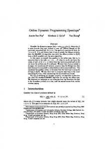
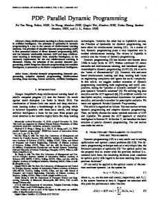
h uh min[( xt1 ,t2 1 xt1 ,t2 )2 , ( xt1 ,t2 1 xt1 ,t2 )2 d , 2 ] (26) v uv [( xt1 1,t2 xt1 ,t2 )2 , ( xt1 1,t2 xt1 ,t2 )2 d , 2 ] (27) On figure 1 show example results of reducing noise MRI with Racian noise level 10 . On figure 2 show example results of reducing noise MRI with Gaussian noise level 15 .
(21)
PSNR (dB) is defined as: 2552 PSNR 10log10 MSE
(22)
SNR (dB) is defined as: M
SNR 10log10 (
N
P(i, j) i 1 j 1
where
MSE
1 M N
M
N
2
1 ) MSE M N
(P(i, j) Q(i, j))
2
;
(23)
P , Q -
i 1 j 1
means of images; P , Q - standard deviations (the square root of variance) of images; P ,Q - covariance of images P (i, j ) 1
Available at http://brainweb.bic.mni.mcgill.ca/brainweb/
Figure 1. Original image (a); Racian noise image (b) with noise level 10 ; denoising results with TV (c), BLSGSM (d), FBF (e), ADF (f), WF (g) , L=2 (h), L=3 (i)
This contribution has been peer-reviewed. doi:10.5194/isprsarchives-XL-5-W6-101-2015
104
The International Archives of the Photogrammetry, Remote Sensing and Spatial Information Sciences, Volume XL-5/W6, 2015 Photogrammetric techniques for video surveillance, biometrics and biomedicine, 25–27 May 2015, Moscow, Russia
Figure 5. Comparison of measurements MSSIM of method with different Rician noise levels
Figure 2. Original image (a); Gaussian noise image (b) with noise level 15 ; denoising results with TV (c), BLS-GSM (d), FBF (e), ADF (f), WF (g) , L=2 (h), L=3 (i)
Figure 6. Comparison of measurements SNR of method with different Gaussian noise levels
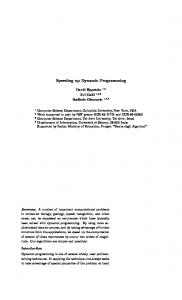
Figure 3. Comparison of measurements SNR of methods with different Rician noise levels
Figure 7. Comparison of measurements PSNR of methods with diffrent Gaussian noise levels
Figure 4. Comparison of measurements PSNR of methods with different Rician noise levels
Results of measurements in figure 3-8 are has been averaged over ten tests. Results show, that our algorithm has the best accuracy to speed ratio, especially in the case of high-resolution images. Details of quantified measurements are showed on figure 3-8 with different Gaussian and Racian noise levels
This contribution has been peer-reviewed. doi:10.5194/isprsarchives-XL-5-W6-101-2015
105
The International Archives of the Photogrammetry, Remote Sensing and Spatial Information Sciences, Volume XL-5/W6, 2015 Photogrammetric techniques for video surveillance, biometrics and biomedicine, 25–27 May 2015, Moscow, Russia
Pattern Analysis and Machine Intelligence, IEEE Transactions, 1984. PAMI-6(6): p. 721 - 741. Hammersley J. M., Clifford P.E., Markov random fields on finite graphs and lattices, 1971. Kalman R. E., Bucy R.S., New Results in Linear Filtering and Prediction Theory. Journal of Basic Engineering, 1961. Vol. 83: p. 95-108 Kopylov, A. et al., 2010. Signal Processing Algorithm Based on Parametric Dynamic Programming. Lecture Notes in Computer Science, Vol. 6134, pp. 280–286.
Figure 8. Comparison of measurements MSSIM of method with diffrent gaussian noise levels
5. CONCLUSION Edge preserving MR denoising has become an urgent step in medical imaging to remove noise and to preserve local image features for an accurate and effective diagnosis. In this paper, we proposed a new approach to achieve these aims. The experimental results show that muti-quadratic dynamic programming procedure with the application of the algorithm kmeans for reduction of the number of executed quadratic functions, allows get the high computational efficiency of dynamic programming for image processing, especially in the case of high-resolution images.
ACKNOWLEDGEMENTS This work was supported by Russian Foundation for Basic Research (RFBR), project № 13-07-00529-a.
REFERENCES Blake A., Zisserman A., 1987. Visual Reconstruction. MIT Press, Cambridge, Massachusetts, 1987, 232 pages. Brown, R. and Hwang, P., 1996. Introduction to Random Signals and Applied Kalman Filtering (3 ed.). New York: John Wiley & Sons, 248 pages. Chaudhury, K., Sage, D. and Unser, M., 2011. , In: IEEE Transactions on Image Processing, Vol. 20(12), pp. 3376 – 3382.
MacQueen J., Some methods for classification and analysis of multivariate observations // Proceedings of 5-th berkeley symposium on mathematical statistics and probability, berkeley, university of california press, 1967.1(281-297). Mottl V., et al., 1998. Optimization techniques on pixel neighborhood graphs for image processing. In: Graph-Based Representations in Pattern Recognition. Computing, Supplement 12. Springer–Verlag/Wien, pp. 135-145. Nikolova M., Michael K., and Tam C.P., 2010. Fast Nonconvex Nonsmooth Minimization Methods for Image Restoration and Reconstruction. In: IEEE Transactions on Image Processing, Vol. 19, no. 12, pp. 3073-3088. Perona, P. and Malik, J., 1990. Scale space and edge detection using anisotropic diffusion. In: IEEE Transactions on Pattern Analysis and Machine Intelligence, Vol. 12. pp. 629–639. Portilla, J., et al., 2003. Image denoising using scale mixtures of gaussians in the wavelet domain. In: IEEE Transactions On Image Processing, Vol. 12, pp. 1338– 1351. Rudin, L., Osher, S., and Fatemi, E., 1992. Nonlinear total variation based noise removal algorithms. In: Journal Physica D, Vol. 60, pp. 259-268. Tomasi, C. and Manduchi, R, 1998. Bilateral filtering for gray and color images. In: proceedings of Sixth International Conference on Computer Vision, pp. 839–846. Xiaojuan G., Li G., 2009. A new method for parameter estimation of edge-preserving regularization in image restoration. In: Journal of Computational and Applied Mathematics, 225, Elsevier, pp. 478-486
Dekker A.J., Sijbers J., 2014. Data distributions in magnetic resonance images: A review, Physica Medica (30),Elsevier, pp. 725-741 Drapaca, C., 2009. A nonlinear total variation-based denoising method with two regularization parameters. In: IEEE Transactions on Biomedical Engineering, Vol. 56(3), pp. 582 – 586. Gerig, G. et al., 1992. Nonlinear anisotropic filtering of MRI data. In: IEEE Transaction on Medical Imaging, Vol. 11 (2), pp. 221–232. Geman S., German D. (1984) Stochastic Relaxation, Gibbs Distributions, and the Bayesian Restoration of Images. In:
This contribution has been peer-reviewed. doi:10.5194/isprsarchives-XL-5-W6-101-2015
106