2007 IEEE International Conference on Robotics and Automation Roma, Italy, 10-14 April 2007
ThB12.1
Multi-Robot Formations based on the Queue-Formation Scheme with Limited Communications Cheng-Heng Fua, Student Member, IEEE, Shuzhi Sam Ge† , Fellow, IEEE, Khac Duc Do, and Khiang Wee Lim, Senior Member, IEEE Abstract— In this paper, we investigate the operation of the Queue-formation structure (or Q-structure) in multi-robot teams with limited communications. Information flow is divided into two time scales: (i) the fast time scale where the robots’ reactive actions are determined based only on local communications, and (ii) the slow time scale, where information required is less demanding, can be collected over a longer time with intermittent information loss. Therefore, there is no need for global information at all times, reducing the overall communication load. In addition, a dynamic target determination algorithm, based on the Q-structure, is used to produce a series of targets that incrementally guide each robot into formation. It provides greater control over the distance between robots on the same queue for better formation scaling. An analysis of the convergence of the system of robots is provided. Simulation studies verify the effectiveness of the scheme. Index Terms— Multi-Robot Formations, Limited Communication Ranges, Deliberative Coordination, Convergence
I. I NTRODUCTION Robust multi-robot collaboration in dynamic and uncertain environments has been intensively studied in recent years. Methods such as virtual leaders [1], social potentials [2] and formation constrained functions [3] can be used to guide robots into formations. Individual robots may also be allocated predefined positions in a formation [4]. A decentralized scheme based on the virtual structure approach has also been proposed for effective formation maintenance [5]. General methods for the controller design for the formation maintenance of multiple vehicles tracking a desired path have also been proposed in [6]. A number of studies have also been carried out on the stability and convergence of formation schemes (largely based on the nodes-and-edges representation) [7]–[9]. Most of the above seminal works use representations based on connectivity graphs where each robot tracks a specific node as a target. Such a representation is also implicit in more reactive approaches, such as those that require a robot to choose and follow a neighbor at a pre-specified distance and orientation. When team size changes, the graph C. Fua is with the NUS Graduate School of Integrative Sciences and Engineering (NGS), at the National University of Singapore. S. S. Ge is with the Electrical and Computer Engineering Department of the National University of Singapore. K. D. Do is with the School of Mechanical Engineering at the University of Western Australia. K. W. Lim is with the Singapore Institute of Manufacturing Technology. †Corresponding author. Tel.: +65 6516 6821; Fax: +65 6779 1103; Email:
[email protected]. This research is partially funded by the A*STAR SERC TSRP GRANT P0520104.
1-4244-0602-1/07/$20.00 ©2007 IEEE.
representation will change and become difficult to track dynamically. Since a large class of problems (e.g. robotic search and surveillance, convoy movements) only require robots to maintain the overall appearance of the formation, the Q-structure has been recently introduced [10] to improve scalability and flexibility. Two drawbacks of the scheme is the reliance on persistent global communications and that the convergence of robots into formations based on the scheme had only been established via experimentation. The main contributions of this paper are as follows: (i) The Q-structure in [10] is extended by considering finite communication ranges, and separating the decision making process into two time scales – a fast time scale for reactive decision making based only on local communications, and a slower time scale which allows less time critical information to propagate through a weakly connected network. Persistent global communications is not required, reducing overall communications load. It also permits intermittent information losses as information is collected over a longer time. (ii) A rigorous proof of convergence for a decentralized control law that guides robots into formations represented by the Q-structure is presented. It extends the work in [11] as follows: (a) Inter-agent potentials are designed to exhibit a different set of properties to reflect limited communication ranges, with a more general controller design, (b) A different, more concise convergence proof for the more general controller is presented. (iii) A dynamic target determination algorithm is proposed to incrementally guide robots into their queues. This improves upon the original scheme [10] by separating agent decisions regarding positions on queues from reactive inter-agent repulsive forces, to an even distribution of agents along queues. II. F ORMATION R EPRESENTATION AND DYNAMIC TARGET D ETERMINATION A. Division of Information Flow Information flow is separated into slow and fast time scales. The control of the formation takes place on these two levels based on the information available on each time scale. (i) Fast-time scale: This facilitates time critical and reactive decision making, such as collision avoidance and getting into formation. It only involves local communications
2385
Authorized licensed use limited to: National University of Singapore. Downloaded on April 5, 2009 at 23:01 from IEEE Xplore. Restrictions apply.
ThB12.1 between robots. Explicit controls governing the actual movements and paths of the agents occur at this level. Such decisions take place at a higher frequency when information is available. (ii) Slow-time scale: This refers to the gradual multi-hop transfer of information, through a weakly connected communication network, between robots not in direct range of each other. The collection of information over a longer time period allows for intermittent information losses between links. Formation control on this level involves low frequency decisions regarding the (re)allocation of robots to different vertices or queues. Interactions between the agents are mostly local since agents respond reactively to data it obtains from others around itself based on direct communication. This is not equivalent to requiring global information at all times for all decisions. (Re)Allocation based on long term information flows occurs at fixed periodic intervals. This information might not be the most current and subjected to time delays. Hence, there is no need for constant global communications between all robots. In addition, while information regarding out-of-range agents may be available, these are not taken into consideration while making pathing decisions other than for (re)allocation.
the long term information propagation through the network. Please refer to [12] for an analysis of the Q-structure using its graphical representation. C. Determination of Target on Queue This section describes an algorithm that each robot ri , associated with a queue Q(i), uses for target determination. The algorithm also governs the distance between robots within the same queue. Compared to the purely reactive scheme in [10], it improves the scaling of formations through an adaptation of the parameter dir (acceptable inter-robot distance for robots on the same queue). Algorithm 1 Determining Target on Queue (by agent ri ) 1: Let Rc,i ∈ RN be an ordered set of agents (according to increasing Euclidean distance from VQ(i) (1)) within communication range of ri and belonging to the same queue as ri , i.e., belonging to Q(i). 2: Suppose ri is the n-th agent in the list Rc,i . 3: if n=1 then 4: Set qtg,i = VQ(i) (1). 5: else 6: Let rj ∈ Rc,i be the (n − 1)-th agent in the list. 7: Set qtg,i = arg min kq − VQ(i) (1)k where Q = {q ∈ q∈Q
B. Formations and Queues For completeness, we briefly state the concepts regarding ‘queues’ and formations as detailed in [10]. Definition 1 (Formations [10]): A formation is a desired overall appearance of the agent team, consisting of relative positioning constraints and acceptable positions for each agent. The constraints are realized in the form of the vertices and queues. A formation is denoted by F = (Q, VF (N )), where Q is the set of queues, and VF (N ) represents the set of formation vertices, Vi (i = 1, . . . , Nv ), where N is the total number of robots1 , around the target. Definition 2 (Queues [10]): A queue, Qj ∈ Q, is denoted as Qj = (Vj , Sj , Cj ). The main elements characterizing a queue are described as follows: (i) Vj ⊆ VF (N ) (Queue Vertices): a list of either one or two formation vertices through which Qj passes. (ii) Sj (Shape): a set of points following an equation in R3 that describes the spatial appearance of Qj , and is specified in the coordinate frame of the first formation vertex in the list Vj . (iii) Cj (Capacity): a fraction that refers to the proportion of the robots in the formation it can hold, i.e., PNall q C j=1 j = 1, where Nq is the total number of queues in the formation. Through the partitioning of information flows into short term and long term flows, we allow reshuffling and refinement of robots between queues (i.e. as per the queue change algorithm presented in [10]) to occur based on long term information gathered from the entire network. The need for robots to react in a timely manner is not compromised by 1 Each formation vertex is represented by its position relative to the coordinate frame of the target.
Q(i) | kq − qtg,j k = dir and kq − VQ(i) (1)k > kqtg,j − VQ(i) (1)k}. The algorithm is executed when Rc,i changes. It works by considering the agents within communication range of ri and which also belong to the same queue as ri . The target of ri is set to be a point on Q(i) and at a distance of dir away from the target of rj . If ri is the agent in Rc,i that is closest to the queue vertex VQ(i) (1), its target will be set to be the queue vertex. The target changes in response to the information it has of other robots within communication range and which are of the same queue. The common objective (FN ) will result in a weakly connected communication network for each subset of agents within the same queue. Although an agent may not be in direct communications with some others within the same queue, the decisions of preceding agents will be reflected by the decisions made by others within communication range. Lemma 2.1: Given a set of agents and considering only direct communications between an agent and those in its neighborhood, Algorithm 1, together with the common objective given in the form of the desired formation FN , will result in constant targets for each agent on each queue. Proof: Let ri and rj be the n-th and (n − 1)-th furthest agents in Rc,i from the queue vertex VQ(i) (1). According to Algorithm 1, if qtg,j is constant, qtg,i will be constant too, and at a distance of dir along the queue from qtg,j . Consider a queue Q∗ where all agents belonging to this queue have converged into a weakly connected net due to the common objective. Let RQ∗ = {rq1 , rq2 , . . . , rqNq } be this set of Nq agents, ordered in ascending order according to their distance from the queue vertex VQ∗ (1). For the set Rc,q1 , rq1 will be
2386 Authorized licensed use limited to: National University of Singapore. Downloaded on April 5, 2009 at 23:01 from IEEE Xplore. Restrictions apply.
ThB12.1 the closest to the vertex, and from Algorithm 1, its target will be constant and locked to qtg,q1 = VQ∗ (1). From the argument in the preceding paragraph, the target of the second agent in RQ∗ , qtg,q2 will be constant because qtg,q1 is fixed. Therefore, by induction, the target of the n − th agent will be fixed and constant, once the agents have converged into a weakly connected net around their respective queues. III. NAVIGATION OF ROBOTS INTO P OSITION From Lemma 2.1, the targets of each agent will become constant within finite time, and the control laws presented in this section will first bring each agent to converge to their queues and onto their desired targets. Consider the following potential function: U = Utg + Uob
(1)
where Utg is the attractive potential between the robots and their target, written as: Utg
(2)
Let a robot, ri , be able to reliably communicate with only Ni robots (comprising the set Ri ∈ R). Uob reflects the collision avoidance behavior, and is chosen to be: Uob =
N −1 X
N X
Uob,ij
i=1
=
≥ 0, if Uij = Utg,ij
(e) Uob,ij ≈ 0, if Uij ≥ 0.5d2ij Based on the above properties, Uob,ij may be chosen as à ! Uij 1 Uob,ij = fij + (6) 2 Utg,ij Uij where fij =
1 1 + exp(at (Uij − Utg,ij )3 )
(7)
where at is a user-defined constant. At each time instant, each robot moves along the negative gradient of the potential function U , given by U˙
=
N X
(qi − qtg,i )T ui
i=1 N −1 X
+
j6=i
0 T Uob,ij qij ui
ΩTi ui
(8)
where qij = qi − qj and Ωi is defined as Ωi
=
N X
(qi − qtg,i ) +
0 Uob,ij qij
(9)
j6=i
This implies that a choice of ui = −CΩi
(10)
where C ∈ Rn+w ×nw is a symmetric, positive definite matrix, which is chosen as C = Inw ×nw c where c > 0, will result in N X (11) ΩTi CΩi U˙ = −
and the closed loop dynamics of a single robot ri in the team is then given by q˙i = −CΩi (12)
If the robots are at non-colliding positions at initial time t0 , and the target of each robot is different as well, these conditions may be written as
(3)
where Uob,ij is a function of Uij and Utg,ij , which are given by 1 Uij = kqi − qj k2 (4) 2 1 kqtg,i − qtg,j k2 (5) Utg,ij = 2 and Uob,ij is chosen such that (a) Uob,ij = ∞, if Uij = 0 (b) Uob,ij > 0, if Uij 6= 0 ∂U 0 = 0, if Uij = Utg,ij (c) Uob,ij = ∂Uob,ij ij ∂ 2 Uob,ij 2 ∂Uij
(qi − qtg,i )T +
N X
i=1
kqi (t0 ) − qj (t0 )k ≥ ²1
i=1 j=i+1
00 (d) Uob,ij =
N X
i=1
N
1X kqi − qtg,i k2 = 2 i=1
=
N X
(13)
where ²1 is a strictly positive constant, and R is the set of robots comprising the team. In addition, Algorithm 1 guarantees that if the condition in (13) is satisfied, the targets for each cycle do not collide, i.e., kqtg,i − qtg,j k ≥ ²2 , ∀i, j ∈ R, where ²2 is strictly positive. It is thus desired that, under such conditions, each robot will converge toward their targets, and at the same time avoiding collisions, i.e. lim (qi (t) − qtg,i ) =
t→∞
kqi (t) − qj (t)k
0
≥ ²3 ,
∀i, j ∈ R and ∀t ≥ t0 ≥ 0 (14)
where ²3 is a strictly positive number representing the minimum acceptable inter-robot distance. Theorem 3.1: Under the conditions (13), the common formation objective, FN , and Algorithm 1, the control input to each robot, given in (10), will result in the convergence of each robot to their desired targets, and such that: (i) The target at qtg is located at an asymptotically stable equilibrium point of (12), and (ii) The critical points of the system other than that at qtg are unstable equilibrium points. Proof: Integrating both sides of (11) from t0 to t, we obtain N N −1 X X Uob,ij (t) Utg (t) + i=1 j=i+1
N X
0 Uob,ij (qi − qj )T (ui − uj )
≤ Utg (t0 ) +
N −1 X
N X
i=1 j=i+1
i=1 j=i+1
2387 Authorized licensed use limited to: National University of Singapore. Downloaded on April 5, 2009 at 23:01 from IEEE Xplore. Restrictions apply.
Uob,ij (t0 )
(15)
ThB12.1 where
loop system in (17) may then be written as Utg (t) Uob,ij (t)
=
1 2
N X
¯ (¯ q¯˙ = −CF q , q¯tg )
kqi (t) − qtg,i k2
i=1
= fij (t)
Ã
Uij (t) 1 + 2 Utg,ij Uij (t)
!
(16)
From the conditions in (13), Uij (t0 ) and Utg,ij are strictly larger than some positive constants. Furthermore, since fij is also bounded (0 < fij < 1), the right hand side of (15) is bounded by some positive constant (the value of which depends on the initial conditions at t0 ). Hence, the left hand side is also bounded, which in turn implies that Uij (t) must be strictly larger than some positive constant for all t ≥ t0 ≥ 0. From (16), kqi (t) − qj (t)k will therefore always be larger than some strictly positive constant, and there will be no collisions. The boundedness of the left hand side of (15) also implies that of kqi (t)k for all t ≥ t0 ≥ 0, and the solutions of the closed loop system in (12) exist. By setting Ωi = 0, we obtain the root sets (critical points) of the system in (12), which are given by q = qtg (due to Property (c) of Uob,ij ) and q = qc (representing the T T ] and remaining critical points), where q = [q1T , . . . , qN T T T T T T qtg = [qtg,1 , . . . , qtg,N ] and qc = [qc,1 , . . . , qc,N ] . The behavior of the equilibrium points is examined by considering the relative distances between agents. To convert the dynamics of each agent (given in (12)) to inter-agent dynamics, we define qij = qi − qj and qtg,ij = qtg,i − qtg,j for all i, j ∈ R for each i, and arranging i and j such that i < j. This yields the dynamics of qij as q˙ij = −CΩij
(17)
Furthermore, given the common formation objective, the system of agents will converge into a weakly connected net, which implies that the maximum distance between any two agents is given by (N − 1)dij , and that q¯ is bounded. Therefore, we have the compact set given by Υ = {¯ q | k¯ q k ≤ N (N − 1)dij }
=
Ωi − Ωj
=
(qij − qtg,ij ) +
where the general gradient of F (¯ q , q¯tg ) with respect to q¯ is ∂F (¯ q , q¯tg ) = ∂ q¯ ∂Ω12 ∂Ω12
=
0 (qij − qtg,ij ) + 2Uob,ij qij
0 Uob,i` qi` −
`6=i
+
N X ¡
`6=i,`6=j
We define: q¯ = q¯tg
=
q¯c
=
N X
0 0 Uob,i` qi` − Uob,j` qj`
¢
(19)
T T T T T [q12 , q13 , . . . , qij , . . . , qN −1N ]
(20)
T T T T T [qtg,12 , qtg,13 , . . . , qtg,ij , . . . , qtg,N −1N ] T T T T T [q12c , q13c , . . . , qijc , . . . , q(N −1)(N )c ]
(21)
.. .
.. . ... .. . ...
.. . ∂ΩN −1N ∂q12
... .. . ∂Ωij ∂qij
.. . ...
... .. . ... .. . ...
∂Ω12 ∂qN −1N
.. .
∂Ωij ∂qN −1N
.. .
∂ΩN −1N ∂qN −1N
(28)
0 00 T = Inw ×nw + 2Uob,ij + 2Uob,ij qij qij
(29)
0 00 = σUob,i + σUob,i q qT ∗ j∗ ∗ j∗ i∗ j∗ i∗ j∗
(30)
in which I(nw ×nw ) is an nw -dimensional identity matrix, and qi∗ j∗ is defined such that (i∗ , j∗ ) 6= (i, j), i∗ 6= j∗ and σ can either be 1 or −1 depending on the values of i, j, i∗ and j∗ . The second and third term in (29) are obtained with the product rule on the second term in (19). Equation (30) is similarly obtained from the third term in (19). To investigate the properties of the equilibrium q¯e , consider the following Lyapunov function candidate Vq¯e = (¯ q − q¯e )T (¯ q − q¯e )
(22)
C¯ = diag(C, . . . , C), (23) F (¯ q , q¯tg ) = [ΩT12 , ΩT13 , . . . , ΩTij , . . . , ΩTN −1N ]T (24)
∂q13
∂Ωij ∂q12
∂Ωij ∂qij ∂Ωij ∂qi∗ j∗
0 Uob,j` qi`
`6=j
∂q12
where i, j ∈ R, and
(18) N X
(26)
upon which LaSalle’s Invariance Principle will be applied to examine the stability of the system around the equilibrium points. To proceed, we linearize (25) at the critical points q¯e , which can be q¯tg or q¯c . This results in ¯ ∂F (¯ q , q¯tg ) ¯¯ d(¯ q − q¯e ) ¯ (¯ q − q¯e ) (27) = −C ¯ dt ∂ q¯ q¯=¯ qe
where Ωij
(25)
(31)
whose derivative along the solution of (31) satisfies
where C¯ comprises E number of C along its diagonal, and E is the total number of communication links that can exist between robots if global communications exist2 . The closed 2 Hence, E may be seen as the number of edges in a fully connected net, with each robot represented as a node.
V˙ q¯e
= −2c
N −1 X
N X
(qij − qe,ij )T
i=1 j=i+1
³
¯ 0 ¯ Inw ×nw + N Inw ×nw Uob,ij q =q ´ ij e,ij ¯ T 00 qe,ij qe,ij (qij − qe,ij ) +N Uob,ij ¯ qij =qe,ij
2388 Authorized licensed use limited to: National University of Singapore. Downloaded on April 5, 2009 at 23:01 from IEEE Xplore. Restrictions apply.
(32)
ThB12.1 ¯ ¯ 0 Since Uob,ij ¯ tuting q¯e =
V˙ q¯tg
¯ ¯ 00 = 0 and Uob,ij ¯
qij =qtg,ij q¯tg into (32)
= −2c
N −1 X
gives
qij =qtg,ij
≥ 2cb(qi∗ j ∗ − qc,i∗ j ∗ )T (qi∗ j ∗ − qc,i∗ j ∗ ) N −1 N X X −2c (qij − qc,ij )T
≥ 0, substi-
i=1,i6=i∗ j=i+1,j6=j ∗
N X
³
T
(qij − qtg,ij )
i=1 j=i+1
³
00 ¯ Uob,ij qij =qtg,ij
¯
Inw ×nw + N
T qtg,ij qtg,ij
´
(33)
i=1 j=i+1
(34)
¡ T qc,ij (qc,ij − qtg,ij )
¯ 0 ¯ + N Uob,ij q
ij =qc,ij
⇒
N −1 X
N ³ X
i=1 j=i+1
=
N −1 X
N X
´ T qc,ij = 0 qc,ij
¯ 0 ¯ 1 + N Uob,ij q
ij =qc,ij
´
c
(35)
i=1 j=i+1
≤ −b
≥ 2bc(q
N X
(qij − qc,ij )T
i=1 j=i+1
¯ 0 ¯ Inw ×nw + N Inw ×nw Uob,ij qij =qc,ij ´ ¯ 00 T ¯ +N Uob,ij q =q qc,ij qc,ij (qij − qc,ij ) ij
c,ij
i∗ j ∗
−q
c,i∗ j ∗
T
) (q
i∗ j ∗
−q
c,i∗ j ∗
(38) ) (39)
which indicates that q¯c is unstable. For practical implementation, a robot ri may not have information from robot out of its communications range and can only compute an approximate value of Ωi , given by X 0 ˆ i = (qi − qtg,i ) + Uob,ij Ω qij (40)
(41)
The approximation error for each robot is = =
ˆ Ω−Ω X
0 Uob,ij qij
(42)
j6=i,j∈Rni
where Rni = R \ Ri is the set of robots that ri cannot communicate with. From property (e) of Uob,ij , we know that for j ∈ Rni , Uob,ij , Uob,ij ≈ 0. In addition, assuming that kqij (0)k is bounded, since the robots converge to their targets on the queues and kqtg,ij k is also bounded, the value of eΩ is bounded by some small positive real value, and the error that arises due incomplete information from robots out of communication range can be kept relatively small through the use of fij to weight the importance of repulsive forces between robots. IV. S IMULATION S TUDIES
(36)
where b is a strictly positive constant. Substituting q¯e = q¯c into (32) gives
³
(qi∗ j ∗ − qc,i∗ j ∗ )T (qi∗ j ∗ − qc,i∗ j ∗ )
ˆ u ˆ˙ = −C Ω
at least one pair (i, j) denoted by (i∗ , j ∗ ) such that
N −1 X
=
eΩ
i j ∗ =qc,i∗ j ∗
(37)
where Ri is the set of robots within the di -neighborhood of ri , and the control law becomes
T qc,ij qc,ij
T qtg,ij and the agents i and j. The agent Consider the term qc,ij j can be seen as an obstacle situated at qij = 0. Similarly, agent i is an obstacle with respect to j at qji = 0. At qij = qc,ij , both agents are at their critical points. For this to hold, both critical points must lie along a straight line along the vector qtg,ij and between qtg,i and qtg,j . That is, the point qij = 0 must lie between the points qij = qtg,ij and qij = qc,ij , and such that these 3 points are colinear. Thus, the NP −1 P N T term qtg,ij is strictly negative and there exists qc,ij
= −2c
ij =qc,ij
´ T qc,ij qc,ij (qij − qc,ij )
j6=i,j∈Ri
T qc,ij qtg,ij
¯ 0 ¯ 1 + N Uob,i ∗j∗ q∗
(qij − qc,ij )T
¯ 00 ¯ N Uob,ij q
Vq¯c V˙ q¯
i=1 j=i+1
V˙ q¯c
N X
(qij − qc,ij )
Considering a subspace such that qij = qc,ij ∀(i, j) ∈ T {1, . . . , N }, (i, j) 6= (i∗ , j ∗ ) and (qij −qc,ij )T qc,ij qc,ij (qij − qc,ij ) = 0, ∀(i, j) ∈ {1, . . . , N }. In this subspace, the following holds
which clearly indicates that q¯tg is asymptotically stable. To show that the remaining critical points of the system (¯ qc ) are unstable equilibrium points, consider the following.
⇒
N −1 X
´
i=1 j=i+1
³
i=1 j=i+1
=0
ij =qc,ij
−2c
(qij − qtg,ij ) N −1 X N X ≤ −2c (qij − qtg,ij )T (qij − qtg,ij )
q¯cT F (¯ qc , q¯tg ) N −1 N X X
¯ 0 ¯ Inw ×nw + N Inw ×nw Uob,ij q
Simulations consist of five circular, omni-directional robots, each of diameter 0.3m, with control input ui in (41) ˆ i in (40). The parameters at , dir and C are chosen using Ω to be 10, 2 and the identity matrix respectively. It is assumed that each robot is able to localize itself in the global frame. Furthermore, each robot is equipped with a laser scanner (180◦ ) and 16 sonar range sensors arranged in a ring around the circular robots for obstacle avoidance. The sensor noise introduced into the range sensing has a normal distribution of 0.2 variance. The communication range of the robots is set to 3m.
2389
Authorized licensed use limited to: National University of Singapore. Downloaded on April 5, 2009 at 23:01 from IEEE Xplore. Restrictions apply.
ThB12.1 25
4.5
A. Formation Convergence and Scaling This section examines the convergence of robots to a wedge formation, and how it scales when 2 robots are removed (deactivated) at t = 10s. In the final formation, robots are to be 2m apart. The robots are initialized at random positions in a 20m×20m square around the point (10m,10m). Figure 1(a) shows how the distance of the robots from their targets vary over time. 4.5
Minimum Distance between robots
Distance between robots and their targets
15
10
5
0
2
4
6
8
10
12
14
10
5
3 2.5 2 1.5 1
0
0
5
10
15
20 25 Time (s)
30
35
40
(a) Convergence of Robots
45
0.5
0
5
10
15
20 25 Time (s)
30
35
40
45
(b) Minimum Inter-Robot Separation
3.5 3 2.5 2 1.5
0.5
0
2
4
Time (s)
6
8
10
12
14
16
18
20
Time (s)
(a) Convergence of Robots
15
3.5
Fig. 2. Robot convergence to formation with formation switching. Wedge: t = [0s, 15s), Column: t = [15s, 30s), Line: t = [30s, 45s)
4
1
0
Minimum separation between robots
Distance between robot and target
4
20
(b) Minimum Inter-Robot Separation
Fig. 1. Robot convergence to formation with robot deactivation/removal at t = 10s.
Figure 1(b) shows the minimum center-to-center distance between any two robots at each time. The minimum distance between any two robots is always greater than 0.5m and no collisions occur. Figure 1(a) shows the distance of each robot from their target at each time instant. The spikes in the graphs are the result of changes in the targets for each robot (according to Algorithm 1) as they interact with others within communication range. These spikes, however, cease to appear when the robots get within communication range of each other and their targets reach a constant state. This is further evidenced by the absence of spikes when scaling occurs at t = 10s, and the robots converge to their new targets. B. Changing Formations This section examines the effect of formation changes from a wedge, to a column (perpendicular to the orientation of the target), and finally to a line (parallel to the target’s orientation). The results are shown in Fig. 2. Spikes are observed in the graphs at the times when formation changes is initiated, occurring due to the abrupt change in targets. Comparing the second and third clusters of spikes, it can be seen that changing from a column to a line is more disruptive due to the further distances to the new targets. On the whole, the team requires an average of transition time of 4 to 6 seconds. V. C ONCLUSIONS In this paper, the original scheme using the Q-structure has been extended to improve the performance when only local
communication is present in a weakly connected network. This is a more realistic environment compared to approaches that require persistent global communications, which is seldom achievable in real world applications. In addition, a dynamic target assignment strategy has been proposed, based on Q-structures, that aims to guide robots into appropriate positions in the required formations. Lastly, we examined the convergence properties of the proposed approach, and further verified the effectiveness of our approach with realistic simulations. R EFERENCES [1] N. E. Leonard and E. Fiorelli, “Virtual Leaders, Artificial Potentials and Coordinated Control of Groups,” Proc. IEEE Conference on Decision and Control, vol. 3, pp. 2968–2973, December 2001. [2] T. Balch and M. Hybinette, “Social Potentials for Scalable Multi Robot Formations,” Proc. IEEE International Conference on Robotics and Automation, pp. 73–80, April 2000. [3] M. Egerstedt and X. Hu, “Formation constrained multi−agent control,” IEEE Transactions on Robotics and Automation, vol. 17, no. 6, pp. 947–951, 2001. [4] A. K. Das, R. Fierro, V. Kumar, J. P. Ostrowski, J. Spletzer, and C. J. Taylor, “A Vision Based Formation Control Framework,” IEEE Transactions on Robotics and Automation, vol. 18, pp. 813–825, 2002. [5] W. Ren and R. W. Beard, “A Decentralized scheme for Spacecraft Formation Flying via the Virtual Structure Approach,” AIAA Journal of Guidance, Control, and Dynamics, vol. 27, no. 1, pp. 73–82, January 2004. [6] W. Kang, N. Xi, Y. Zhao, J. Tan, and Y. Wang, “Formation control of multiple autonomous vehicles: Theory and experimentation,” IFAC 15th Triennial World Congress, pp. 1155–1160, 2002. [7] H. G. Tanner, G. J. Pappas, and V. Kumar, “Leader-to-Formation Stability,” IEEE Trans. on Robotics and Automation, vol. 20, no. 3, pp. 443–455, June 2004. [8] E. Rimon and D. E. Koditschek, “Exact Robot Navigation Using Artificial Potential Functions,” IEEE Trans. Robotics and Automation, vol. 8, no. 5, pp. 501–518, October 1992. ¨ [9] P. Ogren and N. E. Leonard, “Obstacle Avoidance in Formation,” IEEE Int. Conf. Robotics and Automation, pp. 2492–2497, September 2003. [10] S. S. Ge and C. Fua, “Queues and Artificial Potential Trenches for Multi-Robot Formations,” IEEE Trans. Robotics, vol. 21, no. 3, pp. 646–656, August 2005. [11] K. D. Do and S. S. Ge, “Nonlinear Formation Control of Mobile Agents with Collision Avoidance,” Automatica, Submitted October 2005. [12] S. S. Ge, C.-H. Fua, K. D. Do, and K. W. Lim, “Multi-Robot Formations Based on the Queue-Formation Scheme With Limited Communications,” IEEE Trans Robotics, 2006, submitted for review.
2390 Authorized licensed use limited to: National University of Singapore. Downloaded on April 5, 2009 at 23:01 from IEEE Xplore. Restrictions apply.