Multi-sensor Data Fusion Using the Influence Model - MIT Media Lab ...

To Appear: Body Sensor Networks Workshop, Boston MA, April 2006

Multi-sensor Data Fusion Using the Influence Model Wen Dong and Alex Pentland E15-383, 20 Ames Street The MIT Media Laboratory Cambridge, MA, 02139-4307 {wdong, sandy}@media.mit.edu activities, there were 8 × 6 × 7 × 8 = 2688 number of different combinatorial states. As a result, a good algorithm must be able to determine the structural relations between different sensors while avoiding consideration of the exponential number of combinatorial states.

Abstract System robustness against individual sensor failures is an important concern in multi-sensor networks. Unfortunately, the complexity of using the remaining sensors to interpolate missing sensor data grows exponentially due to the “curse of dimensionality”. In this paper we demonstrate that the influence model, our novel formulation for combining evidence from multiple interactive dynamic processes, can efficiently interpolate missing data and can achieve greater accuracy by modeling the structure of multi-sensor interaction.

1. Introduction Multi-sensor networks with tens or even hundreds of sensors are common nowadays. One example of a wearable sensor network is the Groupware systems developed for the DARPA ASSIST program [1]. In this system, data is collected in real-time from several accelerometers, microphones, cameras, and a GPS, all attached to different parts of the soldiers’ clothing. Inference of soldier state is made in real-time, and data automatically shared among different soldiers wearing the Groupwear systems based on the pattern of activity shown among the group of soldiers. A couple of observations from using the Groupware system are worth mentioning. One observation is that sensor failures are unavoidable due to insufficient power supply, sensor faults, connection errors, or other unpredictable causes. This means that an inference algorithm for soldier state must be robust against sensor failures. Another observation is that the data collected from different sensors are often correlated. For example, when the GPS data indicate that a particular person is indoors, this person is also often in a sitting position. This correlation happens in a large combinatorial space. In an early Groupwear system [2] with 8 locations, 6 speaking/non-speaking status, 7 postures, and 8

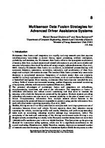
Figure 1. An early Groupware System. Another example of a body-worn sensor network is the cellphone network of the participants of the reality mining project [3]. In this project the 81 participants’ locations, their proximity information, their cellphone usages, and their cellphone states were continuously collected over a period of nine months. As in the Groupware example, the cellphone data collection for the individuals experienced several different types of abnormalities, and the cellphone data for different individuals are correlated. Thus a good data mining algorithm should be robust to abnormalities, and be able to discover the structural relationships among different participants. We believe that our latent structure influence model is an efficient, robust method for analysing these sort of multisensor dynamics problems. It is in the tradition of N-heads dynamic programming on coupled hidden Markov models [4], the observable structure influence model [5], and the partially observable influence model [6], but extends these 1

previous models by providing greater generality, accuracy, and efficiency.

mation is given as follows:

α  ∗t

2. Influence modeling of multi-sensor dynamics The influence model is a tractable approximation of the intractable hidden Markov modeling of multiple interacting dynamic processes. While the number of states of the hidden Markov model is the multiplication of the number of states for individual processes, the number of states of the corresponding influence model is the summation of the number of states for individual processes. The influence model attains this tractability by linearly combining the contributions of latent state distributions of individual processes at time t − 1 to get the latent state distributions of individual processes at time t. Let us assume that we have C interacting stochastic processes and mc (1 ≤ c ≤ C) number of latent states corresponding to process c in the system’s behavior space. Following Asavathiratham [5] we use DC×C as the network (influence) matrix, whose columns each add up to 1, and A(c1 ,c2 ) (1 ≤ c1 , c2 ≤ C) as the inter-process state transition matrix, whose rows adds up to 1. The influence matrix is defined as the Kronecker product H = D ⊗ A = (dc1 ,c2 A(c1 ,c2 ) ) where H is a block matrix whose sub-matrix at row c1 and column c2 is dc1 ,c2 A(c1 ,c2 ) . We express the marginal probabilistic distributions of states (c) st for process c at time t as a row vector consisting (1) (2) (C) of row vectors p(st ) = (p(st ), p(st ), . . . , p(st )), (c) (c) (c) (c) where p(st ) = (p(st,1 ), p(st,2 ), . . . , p(st,mc )), 1 ≤ c ≤  (c) C, j p(st,j ) = 1 is the row vector of the probability distribution on each latent state. Using this notation, the influence process is then p(st+1 ) = p(st ) · H, p(s1 ) = π , so that the marginal distributions at the next time step is a linear combination of the marginal distributions in the current time step. There are many ways to map from an influence matrix H to a master Markov G =   matrix (c ,c) (gi,j ), gs(1) s(2) ···s(C) →s(1) s(2) ···s(C) = c c1 h (c11 ) (c) . t

t

t

t+1 t+1

st

t+1

Nt

=

⎜ ⎜ ⎜ ⎜ ⎝

m P1

i=1

∗(1)

α  t,i

... mC

P

i=1

1 ∗(C)

⎟ ⎟ ⎟ ⎟ ⎠

α  t,i

α  ∗ · Nt t 1P mc ×1 H · diag[bt ]Nt+1 βt+1

α t

=

βt

=

γt

=

t ] α  t · diag[β

ξt−1→t

=

t ] diag[ αt−1 ] · H · diag[bt ] · Nt · diag[β mc  ∗(c) ( α  t,i )

p(o) =

t=T t 1 ⎛ ⎞ 1

(c) (c) T (c) ot  (c)  γt · 1mc ×1 t t

γt,i ot

· δyt ,o(c) ]

(c) T

− μi

(c)

·μ i

3. Experimental Results In this section, we illustrate how an influence model can capture the correlations among different dynamic processes and thus improve the overall classification performance. The noisy body sensor net example illustrates the structure that the influence model tries to capture, and how an influence model can be used to improve classification precision. We then extend the noisy body sensor net example and compare the training errors and the testing errors of different

(c)

represent the observation matrix p(ot ) = p(st ) · B (c) . When the observations for process c are Gaussian, we use nc to represent the dimensionality of the mc number of Gaussian distributions corresponding to each latent state (c) st ∈ [1 . . . mc ]. The EM algorithm for latent state esti2

In the noisy body sensor net example, we have six stochastic processes, and we sample these six processes with six body sensors. Each process can be either signaled (one) or non-signaled (zero) at any time, and the corresponding body sensor has approximately 10% of its samples flipped. The interaction of the six stochastic processes behind the scene looks like this: processes one through three tend to have the same states; processes four through six tend to have the same states; the processes are more likely to be non-signaled than to be signaled; and the processes tend to stick to their states for a stretch of time. The parameters of the model are given as the following and are go .99 .01 , 1 ≤ i, j ≤ 6, ing to be estimated: Aij = .08 .92

 .9 .1 , 1 ≤ i ≤ 6, dij = .33, 1 ≤ i, j ≤ 3, and Bi = .1 .9 dij = .33, 4 ≤ i, j ≤ 6. In Figure 2, (a) shows the sampled latent state sequences, (b) shows the corresponding observation sequences, (c) shows the influence matrix reconstructed from sampled observation sequences, and (d) shows the reconstructed latent state sequences after 300 observations. The (i, j)th entry of the (c1 , c2 )th sub-matrix of an influence matrix determines how likely that process c1 is in state i at time t and process c2 is in state j at time t + 1. It can be seen from Figure 2 (c) that the influence model computation recovers the structure of the interaction. The influence model can normally attain around 95% accuracy in predicting the latent states for each process. The reconstructed influence matrix has only 9% relative differences with the original one. Using only observations of other chains we can predict a missing chain’s state with 87% accuracy.

2 4 6

(d)

500 1000 time step

process id

process id

3.1. Noisy body sensor net example

(c) 1 2 3 4 5 6 1 2 3 4 5 6 process id (a)

2

process id

process id

dynamic models. Finally, we show a wearable sensor net example in which the goal is real-time context recognition, and the influence model is used to discover hidden structure among speech, location, activity, and posture signals in order to allow for more accurate and robust classification of the wearers state.

2 4 6

4 6

500 1000 time step (b)

500 1000 time step

Figure 2. Inference from observations of interacting dynamic processes.

A comparison of different dynamic latent structure models on learning complex stochastic systems 50

testing error (HMM16) testing error (HMM64) 40

error rate (%)

training error (HMM16)

testing error (HMM/chain) 30

training error (HMM/chain) training error (HMM64) training error (influence) 20

testing error (influence) 0

50

100

150

iteration step

Figure 3. Comparison of dynamic models. (c)

the mc = 2 evaluations of “digit” st corresponds a dif(c) (c) ferent 1-d Gaussian observation ot : Digit st = 1 cor(c) (c) 2 responds to ot ∼ N [μ1 = 0, σ1 = 1] ; Digit st = 2 (c) corresponds to ot ∼ N [μ2 = 1, σ22 = 1] . In most real sensor nets we normally have redundant measures and an insufficient observations to accurately characterize sensor redundancy using standard methods. Figure 3 compares the performances of several dynamic latent structure models applicable to multi-sensor systems. Of the 1000 samples (ot )1≤t≤100 , we use the first 250 for training and all 1000 for validation. There are two interesting points. First, the logarithmically scaled number of parameters of the influence model allows us to attain high accuracy based on a relatively small number of observations. This is because the eigenvectors of the master Markov model we want to approximate are either mapped to the eigenvectors of the corresponding influence model, or mapped to the null space of the corresponding event matrix thus is not observable from the influence model, and that in addition the eigenvector with the

3.2. Comparison of dynamic models The training errors and the testing errors of the coupled hidden Markov model, the hidden Markov model, and the influence model are compared in this example. The setup of the comparison is described as the following. We have a Markov process with 2C , where C = 10, number of states and a randomly generated state transition matrix. Each sys(1) (C) tem state st is encoded into a binary st · · · st . Each of 3

largest eigenvalue (i.e., 1) is mapped to the eigenvector with the largest eigenvalue of the influence matrix [5]. Secondly, both the influence model and the hidden Markov model applied to individual processes are relatively immune to overfitting, at the cost of low convergence rates. This situation is intuitively the same as the numerical analysis wisdom that a faster algorithm is more likely to converge to a local extremum or to diverge.

3.3. Real-time Context Recognition An early version of the Groupwear real-time context recognition system was developed by Blum [2], and is comprised of a Sharp Zaurus PDA, an ambient audio recorder, and two accelerometers, worn on hip and wrist (see Figure 1). This system is designed to classify in real time eight locations, six speaking/non-speaking status, six postures, and eight activities. The classification is carried out in two steps: A pre-classifier (single Gaussian, mixture of Gaussians, or C4.5) is first invoked on the audio and accelerometer features to get a moderate pre-classification result of the above four categories. The pre-classification result of different categories is then fed into an influence model to learn inter-sensor structure, and then this learned structure is used to generate an improved post-classification result. In this example the influence model learns the conditional probabilies that relate the four categories (location, audio, posture, and activity) and then uses this learned influence matrix to improve the overall performance. For example, given that the Groupwear user is typing, we can inspect the row of the influence matrix corresponding to “typing” and see that this person is very likely to be either in the office or at home, to not be speaking, and to be sitting. As a result, the action of typing can play a critical role to disambiguating confusions between sitting and standing, or between speaking vs notspeaking, but not between office and home. By combining evidence across different categories using the influence model, the classification errors for locations, speaking/non-speaking, postures, and activities decreased by an average of 23%, from 38%, 22%, 8% and 27% to 28%, 19%, 8%, and 17% respectively. The postclassification for postures does not show significant improvement because of two reasons: (1) it is already precise enough considering that we have labeling imprecision in our training data and testing data, and (2) it is the driving force for improving the other categories, and no other categories are more certain than the posture category.

Figure 4. Influence matrix learned by the EM algorithm.

and latent state estimation algorithms, and demonstrated the latent structure influence model’s superior performance in multi-sensor network analysis.

References [1] 2004. URL http://www.darpa.mil/ipto/ solicitations/open/04-38_PIP.htm. [2] Mark Blum. Real-time context recognition. Master’s thesis, Department of Information Technology and Electrical Engineering, Swiss Federal Institute of Technology Zurich (ETH), 2005. [3] Nathan Eagle and Alex Pentland. Reality mining: Sensing complex social systems. Journal of Personal and Ubiquitous Computing, 2005. [4] Nuria M. Oliver, Barbara Rosario, and Alex Pentland. A bayesian computer vision system for modeling human interactions. IEEE Transactions on Pattern Analysis and Machine Intelligence, (8):831–843, 2000. [5] Chalee Asavathiratham. The Influence Model: A Tractable Representation for the Dynamics of Networked Markov Chains. PhD thesis, MIT, 1996. [6] Sumit Basu, Tanzeem Choudhury, Brian Clarkson, and Alex Pentland. Learning human interactions with the influence model. Technical report, MIT Media Laboratory Vision & Modeling Technical Report #539, 2001. URL http://vismod.media.mit.edu/ tech-reports/TR-539.pdf.

4. Conclusion In this paper, we have presented the formulation of a latent structure influence model, given the parameter learning 4