Multigrid Method for Elliptic Control Problems - NUMA - JKU

JOHANNES KEPLER ¨ T LINZ UNIVERSITA N e t z w e r k f ¨u r F o r s c h u n g , L e h r e u n d P r a x i s

Multigrid Method for Elliptic Control Problems MASTERARBEIT zur Erlangung des akademischen Grades

MASTER OF SCIENCE in der Studienrichtung

INDUSTRIAL MATHEMATICS

Angefertigt am Institut f¨ ur Numerische Mathematik

Betreuung:

O. Univ. Prof. Dipl. Ing. Dr. Helmut Gfrerer Eingereicht von:

Muzhinji Kizito

Linz, August 2008

Johannes Kepler Universit¨ at A-4040 Linz · Altenbergerstraße 69 · Internet: http://www.jku.at · DVR 0093696

This dissertation is dedicated to my wife Wachenuka, our two girls Nyashadzashe and Tapiwanashe, my parents Mr and Mrs Muzhinji, brothers and Sisters, Dr and Mrs Unganai for their support and encouragement. A special dedication goes to my daughter, Tapiwanashe, she was born during the beginning of my two year study and I will see her for the first time when she is already two years old.

Contents Acknowledgements . . . . . . . . . . . . . . . . . . . . . . . . . . . . . . . . . . . . . . . . . . . . . . . . . . .

iv

Abstract . . . . . . . . . . . . . . . . . . . . . . . . . . . . . . . . . . . . . . . . . . . . . . . . . . . . . . . . . . . . .

v

1 Introduction

2

2 ELLIPTIC CONTROL PROBLEMS

5

2.1

2.2

Distributed Control Problems . . . . . . . . . . . . . . . . . . . . . . .

7

2.1.1

Model Problem . . . . . . . . . . . . . . . . . . . . . . . . . . .

7

2.1.2

First Order Optimality Condition . . . . . . . . . . . . . . . . .

8

2.1.3

Lagrange Principle . . . . . . . . . . . . . . . . . . . . . . . . .

9

Boundary Control Problem . . . . . . . . . . . . . . . . . . . . . . . . .

11

2.2.1

Neumann Boundary Control Problem . . . . . . . . . . . . . . .

11

2.2.2

Dirichlet Boundary Control Problem . . . . . . . . . . . . . . .

12

2.2.3

Existence and Uniqueness of the Function Minimum . . . . . . .

13

3 DISCRETIZATION

15

3.1

Variational Formulation . . . . . . . . . . . . . . . . . . . . . . . . . .

15

3.2

Finite Element Method . . . . . . . . . . . . . . . . . . . . . . . . . . .

17

3.2.1

Formulation of the Finite Element Method . . . . . . . . . . . .

17

3.2.2

Finite Elements . . . . . . . . . . . . . . . . . . . . . . . . . . .

20

3.2.3

Assembling of Matrices . . . . . . . . . . . . . . . . . . . . . . .

22

3.2.4

Approximation Properties . . . . . . . . . . . . . . . . . . . . .

24

Discrete Optimality System . . . . . . . . . . . . . . . . . . . . . . . .

27

3.3.1

29

3.3

Integral Equation Characterizing the Optimal Control . . . . .

ii

4 Solution of the Discretized Optimal Control System

31

4.1

Multigrid Algorithm . . . . . . . . . . . . . . . . . . . . . . . . . . . .

31

4.2

Convergence of the Multigrid Method . . . . . . . . . . . . . . . . . . .

35

5 Numerical Results

42

5.1

Test Example 1 . . . . . . . . . . . . . . . . . . . . . . . . . . . . . . .

44

5.2

Example 2 . . . . . . . . . . . . . . . . . . . . . . . . . . . . . . . . . .

49

5.3

Example 3 . . . . . . . . . . . . . . . . . . . . . . . . . . . . . . . . . .

49

5.4

Conclusion . . . . . . . . . . . . . . . . . . . . . . . . . . . . . . . . . .

52

iii

Acknowledgments This work presented so many new challenges during the inceptional and implementational phases. Without the support, patience and guidance of the following people, it would have taken years to be completed. I owe my profound gratitude to the following: 1. Professor Helmut Gfrerer who undertook to act as my supervisor despite his various commitments. Without his support, patience and guidance this work could have been hardly a success. 2. My wife, Wachenuka and our two daughters, Nyashadzashe and Tapiwanashe for allowing me to be away from them for two years of study. My parents Mr and Mrs Muzhinji who always supported, encouraged and prayed for my studies. Above all, a Big Thanks to Dr and Mrs Unganai, without them I could have failed to make it for my studies. 3. My Lecturers both at TU Kaiserslautern(Germany) and Johannes Kepler Linz University(Austria) for providing all the necessary knowledge during the course of my studies. 4. All my friends who were always with and inspired me in this programme. Finally, I would like acknowledge the European Union for financing my studies through the Erasmus Mundus Scholarship.

Muzhinji Kizito Linz, August 2008

iv

Abstract In this work we studied elliptic control problem. It is an optimization problem that consists of the cost functional to be minimized subject to constraints governed by elliptic differential equations with a Neumann boundary condition. We transformed the optimization problem to the optimality system which was characterised in the form of the integral equation on which the multigrid method is applied to find an optimal control. The major goal is to find the optimal control. We achieve this by computing the distributed control problem using finite element method with piecewise linear functions. The domain was partitioned by regular triangulation. The existence and uniqueness of the solutions to the optimal control and the discrete optimal problem is studied and error estimates obtained. Different examples were considered. The convergence of the multigrid method is analysed and the numerical results agree with the theoretical claims.

v

List of Figures Figure

Description

Page

2.1

Model Domain Ω

6

3.1

Initial Mesh and Refinements of Ω

19

3.2

Triangulation of Ω

20

5.1

Example of Refinement Levels

43

5.2

Example 1: Target and Exact Solution

45

5.3

Behaviour of the L2-error

47

5.4

Snapshot of the optimal control at level 4

48

5.5

Desired/Target State at level 4

50

5.6

Example 3: Initial Control and Approximate Control

52

vi

List of Tables Table

Description

Page

5.1

Refinement Levels and Number of Nodes

44

5.2

Convergence results, Error at level 4

46

5.3

Convergence results, Error at level 5

46

5.4

Convergence Results of Different Levels

47

5.5

Convergence Results for Different Weighting Parameter δ

48

5.6

Example 2: Convergence Results at level 4

49

5.7

Example 2: Convergence Results at level 5

49

5.8

Example 3: Control Values at Different levels

50

5.9

Example 3: Convergence Results at level 4

51

5.10

Example 3: Convergence Results at level 5

51

vii

List of Notation and Symbols Symbol

Description

Ω

Solution Domain, Ω ⊂ R2

Ωl

Discrete domain Ωl ⊂ Ω

Γ = ∂Ω

Boundary of Ω

H m (Ω)

 v ∈ L2 (Ω) : ∀α, |α| ≤ m, ∂ |α| v ∈ L2 (Ω)

y, yl

Continuous and discrete state solution

p

Adjoint variable

u, ul

Continuous and discrete control solutions

yd

Desired/target state

A, A⋆

Elliptic differential operators and adjoints

Al , Nl

Stiffness and mass matrices at grid level l

K, Kl

Continuous and discrete integral operators

rl,l−l , pl−1,l

The restriction and the prolongation operators

MGM

Multigrid Method

1

Chapter 1 Introduction An optimal control problem consists of a governing system, a description of the control mechanism, and a criterion defining the cost functional, that models the purpose of the control and describes the cost of its action. The system is governed by the elliptic partial differential equations in our case. The formulation of an optimal control problem involves the cost functional to minimize under the constraint given by the modeling equations. The necessary conditions for such a minimum result in a set of coupled equations called the optimality system. In this and in the next section we describe a control- and a state-constrained optimal control problems. The main thrust of this work is to apply the multigrid method to solve for the constrained optimization problem governed by the partial differential equations. The multigrid method is applied to find the optimal control which is the minimiser of the cost functional. The multigrid method has been shown to be very efficient and successful in solving elliptic control problems(Hachbusch, Borzi). The first step is to transform the optimization problem to the first order optimality system then characterize the first order necessary optimal condition by an integral equation on which the multigrid method is developed, analyzed and finally numerically implemented. The key features of the multigrid method are smoothing and coarse grid correction that involves the inter-grid transfers and a solution correction step. The main results of the work are the convergence of the multigrid method in calculating the control variable. We make numerical experiments for the elliptic control problem

1 δ min(y,u)∈(Y ×U ) J(y, u) = ky − yd k2L2 (Ω) + kuk2L2 (Ω) 2 2 subject to

−∆y + y = f + u ∂y = g ∂n 2

in

Ω

on ∂Ω

(1.1)

The Lagrangian Principle is applied to the elliptic control problem to get the optimal control system(2.13). With u we denote the control function belonging to a set of admissible controls Uad ⊂ U, where U is a real Hilbert space. The state of the system is a function of the control denoted by y(u) ∈ Y , where Y is a real Hilbert space. The optimal control u together with the corresponding state variable y and the co-state/adjoint variable p is the solution of the system

−∆y + y ∂y ∂n −∆p + p ∂p ∂n

= f +u

in Ω

= g

on ∂Ω

= y − yd

in Ω

= 0

on ∂Ω

1 u = − ·p δ

in Ω

Where • y(u) is the solution of the state elliptic partial differential equation corresponding to the control u. • p(u) is the solution of the adjoint elliptic partial differential equation corresponding to the state y(u). • yd is the desired/target state. The state and adjoint solutions depend on the control function u. The control may be involved by the differential equation as above or by the boundary condition. The coupled system is decoupled into an integral equation form(chapter 2 and chapter 3). The decoupling results into a single equation which is not more expensive to solve than the system of elliptic partial differential equations if the fast solver is applied Hachbusch([6], [7]). The optimal control is the solution of the equation of the form

(I − K)u = q where • K is the integral operator(3.34) • I is the identity operator • q is the right hand side involving the yd , f and g. 3

(1.2)

The idea of solving the integral equation characterisation of the optimality system using the multigrid method was used by Hachbusch ( [6] and [7]). The optimal system is discretized using the finite element method. The integral equation replaces the system of elliptic equations on which the multigrid method is applied. The solution of the resulting discrete integral equation is presented in (chapter 5). The two grid method which is the basis of the multigrid is elaborated. The multigrid method algorithm is formulated based on the application of the two grid recursively. The convergence of the multigrid is also analyzed with the main results. In chapter 2 the notion, notations and the several examples of control problems are presented. The finite element discretization which is vital for the assembling of matrices is reviewed in chapter 3 and the characterization of the optimal control by the integral equation including the discretization of the operator. Chapter 4 contains the description of the multigrid method and its properties. The discussion of the numerical solution is presented in chapter 5.

4

Chapter 2 ELLIPTIC CONTROL PROBLEMS The formulation of optimal control of systems governed by elliptic partial differential equations requires the following terms: • The definition of a control function u that represents the driving influence of the environment on the system. • The elliptic partial differential equations modeling the controlled system, represented by the state function y(u). • The cost functional which models the purpose of the control on the system. This work is done on an open domain Ω ⊂ R2 . The domain Ω = (0, 1)2 with boundary ∂Ω = Γ as shown on the figure below.

5

Figure 2.1: Model Domain Ω ∈ R2 with boundary ∂Ω = Γ. The control can be defined in the following ways: Definition 2.1. With reference to the domain figure 2.1 define 1. Distributed Control- if the control is defined on the whole or in some parts of the inside of the domain. 2. Boundary Control- if the control is defined on the whole or parts of the boundary. The examples of the elliptic differential equations for the distributed and boundary control problems are as follows: Distributed Control: Find the state y(u) so that for the given control u ∈ U the following equation is satisfied: Ay(u) = f + u in Ω By(u) = g on ∂Ω

(2.1)

Boundary Control: Find the state y(u) so that for the given control u ∈ U the following equation is satisfied: Ay(u) = f in Ω By(u) = u + g on ∂Ω

(2.2)

This means that y(u) is the solution of (2.1) or (2.2) for a given control u either in the whole domain or on the boundary. A full description of the examples of the distributed and boundary control is given below. Some important notations that are used in the descriptions are given below. 6

• Let A be a differential operator of the second order for example A = (−∆ + I) and A∗ is the adjoint of the operator A. • Let B and C be boundary operators of the first order with smooth coefficients such that the Green’s formula holds

hAy, piL2(Ω) − hy, A⋆piL2 (Ω) = hy, CpiL2(Γ) − hBy, piL2(Γ)

(2.3)

. • Let U be the linear space of control functions that are either distributed(defined on Ω) or boundary(defined on Γ). If U is defined on Γ we have boundary control problem for example the optimal temperature distribution otherwise we have a distributed control problem like the optimal heat source distributed on the whole domain. Define the set of admissible controls Uad ⊂ U. In our case we assume that there are no constraints on the control, then Uad = U. The space of the state, controls and the adjoint are defined on the Sobolev spaces order k, H k , H0k which is the closure of all smooth functions with compact support in Ω(chapter 3)

2.1

Distributed Control Problems

This section involves the study of the examples of the distributed control problems with the boundary condition either Neumann or Dirichlet type. In this case the control is distributed on the whole or on parts of the whole domain Ω. The first order necessary conditions will explicitly be given for the distributed control problems.

2.1.1

Model Problem

The goal is to find the control functions in the domain such that the objective functional is minimized. For this the optimisation problem is defined as: J(y, u) :=

δ 1 k y − yd k2L2 (Ω) + k u k2L2 (Ω) 2 2

(2.4)

which has to be minimized subject to the constraints Ay(u) = f + u in Ω By(u) = g on ∂Ω with 7

(2.5)

1

• f ∈ L2 (Ω) , g ∈ H 2 f ixed and u ∈ Uad = L2 (Ω) varies. • The goal is to get y(u) ≃ yd for a given function yd ∈ L2 (Ω) with the control as small as possible. • The equation (2.5) is called the state equation with the variable y(u) called the state and the yd is the desired/target state. • δ > 0 is the weighting parameter of the cost functional. Since for a given control u we can find the corresponding state y(u), then we can define the control to state mapping S : U → Y, Su := y(u) exists and is continuously differentiable such that the new cost functional will be defined as

F (u) = J(y(u), u) = J(Su, u)

(2.6) (2.7)

This means that S is the solution operator. The new cost functional for the optimization problem is now defined as F (u) :=

1 δ k Su − yd k2L2 (Ω) + k u k2L2 (Ω) 2 2

(2.8)

which has to be minimized

2.1.2

First Order Optimality Condition

Consider the objective function (2.8). The first order optimality condition is given by the theorem below Theorem 2.2. The control u ∈ Uad is optimal if and only if u ∈ Uad and v satisfies the variational inequality hF ′ (u), v − ui ≥ 0 ∀v ∈ U PROOF: Let u ∈ U be the optimal solution and choose v ∈ U By the convexity of Uad we have

wt = u + t(v − u) ∈ Uad 8

∀t ∈ [0, 1].

Now by the optimality of u yields F (wt ) − F (u) ≥ 0 for all t ∈ [0, 1]. Then hF ′(u), v − uiU ⋆ ,U = limt→0

F (u+t(v−u))−F (u) t

≥ 0 On the other hand, using the convexity of F and for all u ∈ Uad we have 0 ≤ hF ′ (u), v − uiU ⋆ ,U = limt→0

F (u+t(v−u))−F (u) t

tF (v) − (1 − t − 1)F (u) t→0 t

≤ lim

= F (v) − F (u). Hence u is optimal control. The multigrid algorithm is applied to find the optimal control of the optimality system(chapter 4). To apply this algorithm we need the adjoint/costate variable which can be found by solving the adjoint elliptic differential equation of the given state partial differential equation. To find the adjoint elliptic partial differential equation, the Lagrangian Principle is used.

2.1.3

Lagrange Principle

In this section we apply the Lagrange Principle to derive the optimality system for the distributed control problem 1 δ J(y(u), u) := k y(u) − yd k2L2 (Ω) + k u k2L2 (Ω) which has to be minimized 2 2 subject to the constraints Ay(u) = f + u in Ω By(u) = g on ∂Ω Introducing the Lagrange multiplier p results in the Lagrange function:
L y(u), u, p = J(y(u), u) − hAy(u) − f − u, piL2 (Ω) − hBy(u) − g, piL2(Γ) = J(y(u), u) − hAy(u), piL2(Ω) + hf + u, piL2(Ω) − hBy(u), piL2(Γ) +hg, piL2(Γ) From the Green’s formula(2.3) we get 9

(2.9)

hAy, piL2(Ω) = hy, A⋆ piL2 (Ω) + hy, CpiL2(Γ) − hBy, piL2(Γ)

(2.10)

This results in the formulation
L y(u), u, p = J(y(u), u) − hy(u), A⋆piL2 (Ω) − hy(u), CpiL2(Γ) + hBy(u), piL2(Γ) +hf + u, piL2 (Ω) − hBy(u), piL2(Γ) + hg, piL2(Γ) = J(y(u), u) − hy(u), A⋆piL2 (Ω) − hy(u), CpiL2(Γ) + hf + u, piL2 (Ω) + hg, piL2(Γ)

This implies that we are looking for the optimality conditions of the linear optimization problem under the assumptions 1. for all u ∈ U there exists a unique y = y(u) such that Ay(u) = f + u in Ω, By(u) = g on ∂Ω 2. Uad is convex, bounded and closed. Theorem 2.3. Let (y(u), u) be an optimal solution then under the assumptions(1-2) there exists a Lagrangian multiplier p such that the optimality system holds • Ay(u) = f + u state equation.
• Ly y(u), u, p = 0 adjoint equation
• hLu y(u), u, p , v − uiU ⋆ ,U ≥ 0 for all v ∈ Uad

From the theorem(2.2), we can observe that u ∈ Uad is an optimal control iff hF ′ (u), v − ui ≥ 0 ∀ v ∈ Uad This means that hy(u) − yd , y(v) − y(u)iL2(Ω) + δhu, v − uiL2 (Ω) ≥ 0 ∀ v ∈ Uad

Now let p(u) be chosen such that A⋆ p(u) = y(u) − yd Cp(u) = 0

in Ω on ∂Ω

(2.11)

and we characterize the optimal control u by

u = −δ −1 p(u) 10

(2.12)

From the relations (2.9), (2.11) and the Green formula(2.3) we get hy(u) − yd , y(v) − y(u)iL2(Ω) = hA⋆ p(u), y(v) − y(u)i
L2(Ω)
= hp(u), A y(v) − y(u) iL2 (Ω) + hp(u), B y(v) − y(u) iL2 (Γ) −hCp(u), y(v) − y(u)iL2(Γ) = hp(u), v − uiL2 (Ω) Since Uad is a linear space,
hp(u) + δu, v − u iL2 (Ω) ≥ 0, ∀ v ∈ Uad We obtain (2.12). Now eliminating u in (2.9) by (2.12) , we get a coupled system of two elliptic partial differential equations. Ay(u) By(u) A⋆ p(u) Cp(u)

= = = =

f − δ −1 p(u) in g on y(u) − yd in 0 on

Ω ∂Ω Ω ∂Ω

(2.13)

A multigrid method is applied to a coupled system(chapter5). The boundary conditions are Neumann type. By and Cp can be replaced by y(u)|Γ and p(u)|Γ to get the analogous results for the Dirichlet problem. The optimality system can be represented in different ways. The next section deals with the representation of the control on the boundary that is the boundary control.

2.2

Boundary Control Problem

This section involves the study of the examples of the boundary control problems with the boundary condition either Neumann or Dirichlet type. In this case the control is restricted on the whole or on some parts of the boundary of the domain Ω. The first order necessary conditions will explicitly be given for the two boundary control problems.

2.2.1

Neumann Boundary Control Problem

The boundary control is an example of the control problem involving an elliptic differential equation with Neumann boundary conditions where the control in defined on ∂Ω. Let y(u) be defined by Ay(u) = f in Ω By(u) = u + g on ∂Ω for u ∈ Uad = U = L2 (Γ). The cost functional δ 1 k y(u) − yd k2L2 (Ω) + k u k2L2 (Γ) 2 2 2 which has to be minimized where yd ∈ L (Ω) is the target state. J(y(u), u) :=

11

(2.14)

The optimal control is defined on the boundary and is given by

u = −δ −1 p(u)|Γ

(2.15)

where p(u) is the solution of the adjoint elliptic differential equation(2.11). The resulting optimality system

Ay(u) By(u)|Γ A⋆ p(u) Cp(u)

= = = =

f g − δ −1 p(u)|Γ y(u) − yd 0

in on in on

Ω Γ Ω Γ

(2.16)

The system above describes the behaviour on the boundary. The other way in which the boundary control problem with Neumann boundary condition can be represented is: Consider the cost functional which describes the behaviour on the boundary 1 δ k y(u) − yd k2L2 (Γ) + k u k2L2 (Γ) 2 2 2 which has to be minimized where yd ∈ L (Γ) is the target state. J(y(u), u) :=

Let y(u) fulfils the state equation ( 2.14) with (2.15) yields the optimal control provided p(u) solves the adjoint partial differential equation A⋆ p(u) = 0 Cp(u)|Γ = y(u)|Γ − yd

in Ω on Γ

(2.17)

Then the resulting optimality system becomes Ay(u) By(u)|Γ A⋆ p(u) Cp(u)|Γ

= = = =

f in −1 g − δ p(u)|Γ on 0 in y(u)|Γ − yd on

Ω Γ Ω Γ

(2.18)

which is a coupled by the boundary condition.

2.2.2

Dirichlet Boundary Control Problem

Let the target/desired state yd ∈ L2 (Ω) and the set of admissible controls defined as Uad = U = L2 (Γ). Let y(u) be defined by Ay(u) = f in Ω y(u) = u + g on ∂Ω The cost functional J(y(u), u) :=

δ 1 k y(u) − yd k2L2 (Ω) + k u k2L2 (Γ) 2 2 which has to be minimized. 12

(2.19)

The optimal control on the boundary is given u = −δ −1 p(u)|Γ where p(u) is the solution of the adjoint elliptic differential equation. A⋆ p(u) = y(u)|Γ − yd p(u) = 0

in Ω on Γ

(2.20)

in on in on

(2.21)

Then the resulting optimal system becomes Ay(u)) y(u)|Γ A⋆ p(u) p(u)

= = = =

f g − δ −1 p(u)|Γ y(u)|Γ − yd 0

Ω Γ Ω Γ

which is a coupled by the boundary condition.

2.2.3

Existence and Uniqueness of the Function Minimum

In this section, the existence and uniqueness of the control function as the minimizer of the cost functional is analyzed. We have the cost functional J(y(u), u) with J : Y × U −→ R is investigated with y(u) and u related by the operator S : U −→ Y. With the new cost functional defined by (2.6, 2.7, 2.8). Theorem 2.4. (Existence of the minimiser) Let U be a Hilbert space, Uad ⊂ U non-empty, bounded, closed and convex and F : U −→ R weakly lower semi-continuous and U radially unbounded, that is 1. un ⇀ u⋆ follows that F (u⋆ ) ≤ lim inf n→∞ F (un )(Weakly lower semi-continuous). 2. k u k−→ ∞ follows that F (u) −→ ∞.(radially unbounded) With linear and bounded operator S, assume F is bounded from below by a constant C ∈ R with C ≤ F (u) ≤ ∞ for u ∈ U. Then the minimization problem minu⋆ ∈Uad F (u) has a solution u⋆ ∈ Uad .

PROOF. Let F be bounded from below, it implies the existence of the infimum. This means that there is a sequence (un ) ⊂ Uad with F ⋆ = limn→∞ F (un ). By the radial unboundedness of F , (un ) is bounded, and there exists a weakly converging subsequence (unk ) of un such that 13

unk ⇀ u⋆ as k → ∞. Since Uad is closed and convex subset of the Hilbert space it is weakly closed and hence u⋆ ∈ Uad . Since S is linear and bounded, it follows weak convergence in Y; Sunk ⇀ Su⋆ as k → ∞. Due to weakly lower semi continuity of F we obtain F (u⋆ ) ≤ lim inf n→∞ F (unk ) = F ⋆ f or k → ∞. Since F ⋆ is the infimum if and only if F (u⋆ ) = F ⋆ Hence the minimum is attained at u⋆ . Theorem 2.5. (Uniqueness) Let the conditions of theorem(2.4) holds. If additionally F is strictly convex, then there exists at most one optimal control.

14

Chapter 3 DISCRETIZATION This chapter deals with the discretization of the optimization model(optimality system(2.13)) problem, distributed control by the finite element method. The ingredients of the finite element discretization are the variational formulation where the test spaces are introduced, the existence and uniqueness of the solution. The finite element method described here is based on the references (Braess([3]), Knabner and Angermann([11])). The convergence, stability and the approximation property of the solution are also going to briefly discussed. The discretization of the optimality system and finally the discretization of the operator K of the integral equation characterisation of the optimality system are also going to be demonstrated. In this chapter the Galerkin method is used to discretize the distributed control problem (2.4, 2.5) with Neumann boundary ∂ condition. From now on we assume that A = −∆ + I and B = ∂n .

3.1

Variational Formulation

Assuming the existence of a classical solution, the following steps are performed in general: • Step 1: Multiplication of the differential equation by test functions that are chosen compatible with the type of boundary condition and subsequent integration over the domain Ω. • Step 2: Integration by parts and incorporation of the boundary conditions in order to derive a suitable bilinear form. • Step 3: Verification of the required properties like ellipticity and continuity(Knaber and Angermann([11])). The solution of the elliptic differential equation is based on the weak formulation in the Sobolev spaces.

We demonstrate the variational formulation of the state partial differential equation and that for the adjoint follows immediately.

15

We choose the test function w ∈ W = H 1 , multiply by the test function and integrate by parts Z R (−∆y + y) · wdx = Ω (f + u) · wdx ZΩ Z Z R ∇y · ∇wdx − (∇y · n)wds + y · wdx = Ω (f + u) · wdx Ω

Z

Γ

∇y · ∇wdx +

Ω

Z

Ω

y · wdx

=

Ω

R

Ω

(f + u) · wdx +

R

Γ

g · wds

Define • the bilinear form a : H 1 × H 1 −→ R Z Z a(y, w) = ∇y · ∇wdx + y · wdx Ω

(3.1)

Ω

• the linear form

F (w) =

Z

F : H 1 −→ R (f + u) · wdx + Ω

Z

g · wds

(3.2)

Γ

• The variational formulation Find y ∈ H 1 such that a(y, w) = F (w) ∀w ∈ W = H 1

(3.3)

Definition 3.1. Let W be a Hilbert space. A bilinear form a : W × W −→ R is called: • symmetric if a(y, w) = a(w, y)

∀w, y ∈ W.

• continuous if |a(y, w)| ≤ C k y kW · k w kW . • coercive if a(w, w) ≥ γ k w k2W . The variational formulation for the adjoint and the state elliptic partial differential equations for the distributed optimal control system(2.15, 2.16), for the given control u a(y(u), w) = hf + u, wiL2(Ω) + hg, wiL2(Γ) a(w, p(u)) = hw, y(u) + yd iL2 (Ω)

for all w ∈ W = H 1 for all w ∈ W = H 1

In this work we consider a(y(u), w) = a(w, p(u)), so it will be enough to assemble a(y(u), w). The central theorem the ensure the unique solvability of the variational problem is the Lax Milgram theorem which holds for convex sets. 16

Theorem 3.2. The Lax Milgram Theorem Let W be a Hilbert space. Let a : W × W −→ R be a continuous, coercive bilinear form and F : W −→ R a linear functional. Then the variational equation

a(y, w) = F (w)

for all w ∈ W

(3.4)

has a unique solution y ∈ W . Moreover, the solution satisfies the estimate

k y kW ≤

3.2

1 k F kW ⋆ γ

(3.5)

Finite Element Method

In this section we discuss the finite element discretization of our domain Ω = (0, 1)2 . This can be achieved with the following general steps. 1. Discretize the domain Ω, that is to divide the solution region into finite elements(subdomains). The solution domain is divided into several simpler finite elements, where each element has a simple geometry, so appropriate assumed solutions can easily be written for the element. In this thesis the sub-domains are the triangles. 2. Establish the matrix equation for the finite element which relates the nodal values of the unknown function to other parameters. In this work we use the Galerkin method. 3. To find the global equation system for the whole solution, all element equations must be assembled. This involves the combination local element equations for all elements used for discretization. The Neumann boundary condition is incorporated on the right hand side 4. Solving the global equation system. Since the finite element global equation system is typically sparse, symmetric and positive definite, direct and iterative methods can be used for the solution. In this work the multigrid method which is an iterative solver is used. The nodal values of the sought function are produced as a result of the solution, since approximating functions are determined in terms of nodal values of as physical field which is sought.

3.2.1

Formulation of the Finite Element Method

As we have mentioned in (1-4) above, several approaches can be used to transform the physical formulation of the problem to its finite element discrete state. Since the formulation of the problem is described by an elliptic differential equation then the most popular method of its finite element formulation is the Galerkin method. 17

The Galerkin Method The Variational Problem of the model problem is given by Find y ∈ W : a(y, w) = F (w), where

∀w∈W

• W is the solution space with W = H 1 • a(., .) is a continuous bilinear form on W × W . • F (.) is a continuous linear form on W . The idea is to replace the infinite dimensional space W by a finite dimensional space Wh ⊂ W which consists of a fixed degree associated with the subdivisions of the computational domain. Let Hl for l ∈ N0 be a sequences of subspaces of the finite dimensional subspace Wh defined on each level of refinement l. Hl ⊂ Hl+1 ⊂ Wh ⊂ W = H 1 where Hl+1 subspace which correspond to Ωl+1 is the refinement of Ωl with subspace Hl such that Ωl ⊂ Ωl+1 ⊂ Ω. An example is illustrated in the figure below where Ω0 is the initial mesh l = 0 and Ω1 is a refinement of Ω0 as shown on the figure below

18

Figure 3.1: Left: Initial Mesh Ω0 , Right: One Refinement Ω1 Now consider the variational problem in the finite dimensional subspace

Find yl ∈ Hl : a(yl , wl ) = F (wl ),

∀wl ∈ Hl

Suppose that the dimHl = Nl and to calculate the solution we choose the basis functions which are linearly independent with a small support n o Hl = span φ1 , φ2 , ..., φNl Now expressing the approximate solution yl in terms of the basis functions l yl = ΣN i=1 ξi φi

ξi ∈ R i = 1, 2, ..., Nl

Then the new variational problem reads

19

Find ξ = (ξ1 , ξ2, ..., ξNl ) ∈ RNl :

l ΣN i=1 a(φj , φi )ξi = F (φj ) j = 1, ..., Nl

(3.6)

This is a linear system of equations for ξ = (ξ1 , ξ2 , ..., ξNl )T with matrix Al = a(φj , φi) ∈ RNl ×Nl and bj = F (φj ) ∈ RNl ×1 Since φi have small support, a(φj , φi ) = 0 for most i and j the matrix Al is sparse(most of the entries are zeros). Lemma 3.3. Let a be a coercive, bilinear form then the matrix Al is positive definite. A symmetric bilinear form implies symmetry of matrix Al .

3.2.2

Finite Elements

In this section the construction of the Finite Element method is described. Let Hl ⊂ Wh consists of continuous piecewise linear functions. Let Ω = (0, 1)2 be a bounded domain, with boundary ∂Ω = Γ. The domain Ω can be covered with a finite number of triangles as shown on the figure below

Figure 3.2: An example of a triangulation

20

The subdivision of the domain into triangles is called triangulation. Definition 3.4. (Triangulation) n o Let Ω ⊂ R2 . A partition Th = T1 , T2 , ..., TN of Ω into triangular elements is called admissible provided the following properties hold 1. Ω = ∪T ∈Th T . 2. if Ti ∩ Tj consists of exactly one point, then it is a common vertex of Ti and Tj . 3. if for i 6= j, Ti ∩ Tj consists of more than one point, then Ti ∩ Tj is a common edge of Ti and Tj . Where h := max1≤i≤N diam(Ti ) denotes the maximum diameter of all T ∈ Th . The items 2 and 3 implies that Ti and Tj are adjacent. With each node we associate the basis function φ which is equal to 1 at the node and 0 at all other nodes. For example at node xj , we have that

φi (xj ) =



1 if i = j 0 if i 6= j

φ is assumed to be a continuous function on Ω and linear on each of the triangles. Suppose that the nodes are labeled 1, ..., Nl and let φ1 (x, y), ..., φNl (x, y) be the corresponding basis functions. The functions φ1 , ..., φNl are linearly independent and span a Nl dimensional linear subspace Hl at level l. For our the model problem the finite element can be restated as

Find ξ = (ξ1 , ξ2, ..., ξNl ) ∈ RNl : Z

∂φi ∂φj ∂φi ∂φj ( + + φi φj )ξi dxdy = ∂y ∂y Ω ∂x ∂x for j = 1, ..., Nl . l ΣN i=1

Z

Ω

(f + u)φj dxdy +

Z

gφj ds

∂Ω

Letting Al = (aij ) and bl = (F1 , ..., FNl )T where • aij = aji = • bj =

R

Ω

R  ∂φi ∂φj Ω

∂x ∂x

+

∂φi ∂φj ∂y ∂y

 + φi φj dxdy


R f + u φj dxdy + ∂Ω gφj ds

The finite element approximation can be written as a system of linear equation Al ξ = bl 21

(3.7)

3.2.3

Assembling of Matrices

In subsection(3.2.2), we have developed a system of equations. We now want to calculate each of these terms involved in these systems. It is important to note that each φi defined in the previous subsection has support over at most two elements thus when a regular triangulation Th has been generated for the domain, we can calculate the stiffness matrix Al , the mass matrix Nl and the right hand side bl which is the sum of f l and gl at each level l. For the stiffness matrix and the mass matrix we have

Aij =

P

T ∈Th

R

∇φi ∇φj dx,

T

Nij =

R

P

T ∈Th

T

φi φj dx

and for the right hand side we consider the construction of f and g.

fj =

P

T ∈Th

R

T

f φj dx and gj =

P

T ∈Th

R

E

gφj ds

Definition 3.5. The local stiffness and mass matrices ATl , NlT ∈ R3×3 are defined by Z (T ) (Al )ij = ∇φi ∇φj dx for i, j = 1, 2, 3 (3.8) T

(T ) (Nl )ij

=

Z

φi φj dx

for i, j = 1, 2, 3

(3.9)

T

For a triangular element T ∈ Th , with vertices (x1 , y1 ), (x2 , y2 ), (x3 , y3) and φ1 , φ2 , φ3 be the corresponding basis functions in Hl . We denote the area of the triangle by |T | with

1 1 1 |T | = x1 x2 x3 y1 y2 y3

Since 

  −1   φ1 (x, y) 1 1 1 1  φ2 (x, y)  =  x1 x2 x3   x  φ2 (x, y) y y1 y2 y3 It can easily be computed that   1 yi+1 − yi+2 ∇φi (x, y) = 2 xi+2 − xi+1 22

indices are modulo 3

(3.10)

(3.11)

Then

 yj+1 − yj+2 yi+1 − yi+2 xi+2 − xi+1 xj+2 − xj+1 R This means that we get the local stiffness matrix for the term T ∇φi ∇φj dx. This can be expressed as (T )

Al

Z

=




1 ∇φi ∇φj dx = 4|T | T

|T | 2



· Grad · GradT where the  −1   0 0 1 1 1 Grad =  x1 x2 x3   1 0  0 1 y1 y2 y3

Now for the mass matrix which is from the term we get (T )

Nl

=

|T | (1 12

R

T

(3.12)

φi φj dx. Using the quadrature rule

+ δij ) i, j = 1, 2, 3

which is (T )

Nl



 2 1 1 |T |  1 2 1  = 12 1 1 2

(3.13)

After computing the element stiffness and mass matrices we sum over all the elements to obtain the global matrices. As mentioned already above the stiffness and the mass matrix for the state and the adjoint equations take the same form.

The Right Hand Side Since we are going to apply the multigrid method to a system of elliptic partial differential equations, we need only to assemble the desired state. The solution procedure will require us to input the initial control into the state equation, solve for the state, input the state into the adjoint equation and finally find the optimal control. To assemble R for the desired state, we use the quadrature rule. To assemble the term involving y φ dx. This can be written as Ω d,l j Z XZ yd,l φj dx (3.14) yd,l φj dx = Ω

T ∈Th

T

R We approximate the integral T yd,l φj dx using the midpoint rule such that (xs , ys ) is the centroid of each element. Numerical realization of this term also in the simplest case involves one point numerical quadrature. The integral can be evaluated as Z |T | yd,l φj dx = yd,l (xs , ys ) (3.15) 3 T And this is the same as multiplying the element mass matrix by the value of yd,l at the nodes. (T ) (yd,l )(T ) = Nl · yd (xi , yi) i = 1, 2, 3 (3.16) 23

R To assemble the term involving Ω fl φj dx. This can be written as Z XZ fl φj dx fl φj dx = Ω

T ∈Th

(3.17)

T

R We approximate the integral T fl φj dx using the midpoint rule such that (xs , ys ) is the centroid of each element. This can be written as Z XZ f (xs , ys )φj dx (3.18) fl φj dx = Ω

T

T ∈Th

Numerical realization of this term also in the simplest case involves one point numerical quadrature. The integral can be evaluated as Z |T | fl (xs , ys ) (3.19) fl φj dx = 3 T Now for the boundary term gj =

XZ

T ∈T

gl φj ds

(3.20)

E

where E is the edge of one of the element. Let (xm , ym) be the midpoint of the edge. Then the integration over the edge yields Z gl φj ds ≃ gl (xm , ym )|E| (3.21) E

where |E| is the length of the edge.

3.2.4

Approximation Properties

In this section, having established the construction of the finite element for the state and the adjoint elliptic equation, now we establish approximation properties of our solutions. We have the variational formulation for the state and the adjoint elliptic partial differential equations a(y(u), w) = hf + u, wiL2(Ω) ∀w ∈ H 1 a(w, p(u)) = hw, y(u) − yd iL2 (Ω) ∀w ∈ H 1 We keep in mind that the two equations have the same bilinear a(., .) form which is W − elliptic, continuous and symmetric. Let Hl for l ∈ N0 be a sequence of subspaces with

24

Hl ⊂ Hl+1 ⊂ H s

s ≥ 1.

In our case s = 1. Then the discrete solutions at each level of discretization is defined by Definition 3.6. Find discrete solutions yl (v), pl (v) ∈ Hl such that

a(yl (v), wl ) = hfl + v, wl iL2 (Ω) ∀wl ∈ Hl a(wl , pl (v)) = hwl , yl (v) − yd,l iL2 (Ω) ∀wl ∈ Hl

(3.22) (3.23)

This means that at each level, we can compute the discrete solutions for the state, adjoint depending on the discrete control vl . The subspaces Hl are connected by the step size hl and the approximation property. To begin the approximation property is the C e´a’s lemma in the general subspace.. Lemma 3.7. Let the bilinear form a : W × W → R be continuous and W-elliptic. Suppose y and yh are the solutions of variational formulation in W and Wh ⊂ W respectively then

k y − y h kW ≤

C infwh ∈Wh k y − wh kW γ

PROOF: by the definition of y and yh a(y, w) = F (w) a(yh , w) = F (w)

∀w ∈ W ∀w ∈ Wh

Since Wh ⊂ W , by subtraction

a(y − yh , w) = 0

∀w ∈ Wh

Galerkin Orthogonality

Let wh ∈ Wh with w = wh − yh ∈ Wh ⊂ W , then

a(y − yh , wh − yh ) = 0 and by coercivity and continuity γ k y − yh k2W ≤ a(y − yh , y − yh ) = a(y − yh , y − wh ) + a(y − yh , wh − yh ) ≤ C k y − yh kW · k y − wh kW ∀wh ∈ Wh hence dividing by k y − yh kW the result follows. 25

(3.24)

• The C e´a’s lemma says that the accuracy of the numerical solution depends on the choice of the function spaces which are capable of approximating the solution y. • The choice of Wh is important. Let the space Wh be a space of linear piecewise finite elements

 Wh = y ∈ C 0 (Ω) : y|Ti ∈ P1 , Ti ∈ T • The error estimates are primarily based on the estimating the approximation error infwh ∈Wh k y − wh kW . • From the C e´a’s lemma the discretization error is estimated by the approximation error which is estimated by the interpolation error Let the continuous solution be regular enough, that is y ∈ H 2 (Ω). Now for arbitrary w ∈ H 2 (Ω) define the interpolation operator

Πh : H 2 (Ω) → Wh w 7→ Πh w Hence it follows that infwh ∈Wh k y − wh kH 1 ≤k y − Πh y kH 1

(3.25)

As a consequence, it is enough to deal with the interpolation error k y − Πh y kH 1 for convergence results. The main ideas are 1. localise the error on the triangles(elements) 2. transformation of the triangles on the reference triangles. 3. compute the local interpolation error. 4. inverse transformation back to the triangles(elements). Following the ideas 1-4 above, the interpolation error in our case is given by the theorem Theorem 3.8. Let y ∈ H 2 (Ω) with Ω = (0, 1)2. Then the interpolation error satisfies

k y − Πh y kH 1 ≤ Ch k y kH 2 26

Then the convergence follows from the C e`a’s Lemma. Theorem 3.9. Let T a quasi-uniform triangulation of Ω. Let y and yh be the solutions of the continuous and discrete variational equations respectively. Then for y ∈ H 2 (Ω).

k y − yh kH 1 ≤ Ch k y kH 2

(3.26)

Where C is independent of the level l This gives the convergence in H 1 -norm. This means that there is a linear convergence for finite element error in H 1-norm, that is k y − yh kH 1 = O(h) Similarly, the convergence in L2 -norm follows for the Aubin-Nitsche theorem on shape regular triangulation. Theorem 3.10. (Aubin-Nitsche) Suppose that Ω is a convex polygon and that Th is regular family of meshes on Ω. Then

k y − yh kL2 (Ω) ≤ Ch2 k y kH 2

(3.27)

for some constant C > 0 This implies that we have a quadratic convergence for the finite element in L2 -norm, that is k y − yh kL2 (Ω) = O(h2 ). Hence for our case the following stability estimates are valid for f = yd = 0 and g = 0

k yl (u) kH 1 (Ω) ≤ C k u kL2 (Ω) k pl (u) kH 4 (Ω) ≤ C k yl (u) kH 1 (Ω)

3.3

Discrete Optimality System

For the optimization problem there are two ways: first optimize, then discretize or first discretize, then optimize(Hinze[10]). In this work the approach is optimize the optimization problem then discretize. The continuous optimal system(2.17) was transformed into the discrete optimal system by discretization using finite element method. Consider a sequence of discretizations with different step sizes h and level of refinement l. Fix the coarsest grid size h0 and define hl = 2−l h0

l ∈ N0 = 0, 1, 2, ... 27

where l is the level number. The discrete optimal system resulting from the Galerkin method is min(yl ,ul )∈L2 ×L2 J(yl , ul ) =

δ 1 k yl − yd,l kL2 (Ω) + k ul k2L2 (Ω) 2 2

(3.28)

subject to the constraints Al yl + Nl yl = Nl fl + Nl ul Al pl + Nl pl = Nl yl − Nl yd,l 1 Nl ul = − Nl pl δ

(3.29) (3.30) (3.31)

where Al and Nl are the stiffness and mass matrices at level l respectively. Remark 3.11. The state and adjoint elliptic partial differential equations have the same stiffness and the mass matrices at each level The idea is to solve a set of constraints for the values of the state and the control that minimise the objective function. Then the solution procedure is defined as follows(Hackbusch[6]) 1. choose the initial control u0 2. find yl = Su0 , solve the elliptic state equation, where S involves Al and Nl . 3. find pl = S ⋆ (yl − yd,l ) 4. find ul = − 1δ · pl 5. where S is the solution operator with S = S ⋆ 6. set u0 = ul and go to (1) with the multigrid method coming into play. From (1-6) above it means that we can calculate the discrete state yl (vl ) from the discrete control vl and the discrete adjoint pl (vl ) from the discrete state yl (vl ). Then we can define the optimal discrete control ul for the distributed control problem as

ul = −δ −1 · pl (vl )

(3.32)

The whole set of constraints of our discrete optimal control system (3.28 - 3.30)can be expressed as a matrix system      Al + Nl O −Nl yl Nl fl  −Nl Al + Nl O   pl  =  −Nl yd,l  (3.33) O Nl δNl ul O This defines the matrix equation of our solution procedure for the optimal control. The formulation(3.33) can be characterized by an integral equation. 28

3.3.1

Integral Equation Characterizing the Optimal Control

The Operator K The mapping u 7→ y(u) 7→ p(u) 7→ −δ −1 p(u) is affine and defined on a linear operator K such that the optimal control(2.15) can have the representation −δ −1 p(u) = Ku + q

(3.34)

This defines the solution procedure(Hackbusch[6]). The operator K is a linear operator. The operator K or the powers of K map into the space with finer topology. The powers of K signifies the number of times the operator K is applied in the solution process. Let B0 and B1 ⊂ B0 be two Banach spaces, where B1 is finer than B0 . K m has to satisfy k K m kB0 →B1 ≤ C, m ≥ 1 f ixed In Ref.(5), for the choices of the two Banach spaces B0 and B1 for the distributed control equation(2.15, 2.16). Let u ∈ L2 (Ω) implies that y(u) ∈ H 2 (Ω) and p(u) ∈ H 4 (Ω), if Γ and the coefficients are smooth. If m = 1, B0 = L2 (Ω), B1 = H 4 (Ω). This means that more generally, K m : L2 (Ω) → H 4m (Ω) continuous f or all m ≥ 1 For the other examples 1. Considering the Distributed control with Dirichlet boundary condition K m : L2 (Ω) → H m (Ω) continuous 2. the Neumann boundary control problem(2.19) K m : L2 (Γ) → H 3m (Γ) continuous 3. Considering the Boundary control with Dirichlet boundary condition(2.24) K m : L2 (Γ) → H m (Γ) continuous The discrete optimality system (3.28 - 3.31 ) is going to be solved using the multigrid method. Let the discrete control vl , discrete state and the adjoint yl (vl ), pl (vl ) and the desired control ul . The discrete optimality system(3.33) simplifies to h i 1 −1 N A N (u + f ) − y Nl ul = − Nl A−1 l l l l d,l l l δ

29

(3.35)

Definition 3.12. (Discrete Integral Equation) The discrete optimality system(3.28 - 3.30) is equivalent to the discrete integral equation (Il − Kl )ul = ql

(3.36)

with 1 Nl (A−1 Kl = − A−1 l Nl ) δ l i 1 −1 h −1 Al Nl Al Nl fl − yd,l ql = δ Kl is the discrete operator of K. The knowledge of the entries of the matrix K is not necessary except at the coarsest level(l = 0). The similar approach can be used to derive the analogous discrete integral equation for the boundary control problem. In Hachbusch([6]), the most important requirement for Kl is that k Klm kB0l →B1l ≤ C, l ∈ N0 . This will be applied in the next in chapter 4, on the convergence analysis of the multigrid method. The solution of the discrete integral equation is clearly the optimal control. To solve the discrete system the multigrid method(chapter 4) is applied.

30

Chapter 4 Solution of the Discretized Optimal Control System In this chapter we want to develop a multigrid algorithm for solving the discretized optimal control system. The main goal being to find the pair (yl , ul ) of the discrete control and the discrete state variables at the finest level l. To calculate this, an multigrid algorithm is developed over the discrete integral equation that characterizes the discrete optimal control. As has been already been highlighted in section(3.3.1), the discrete optimal constraints are reduced to one system of elliptic equations. So the multigrid algorithm will require only the numerical solution of a sequence of single elliptic equations. The optimal control can be obtained by solving one system of two elliptic equations. In this work we will illustrate the numerical treatment of a discrete optimal control problem by applying the multigrid method(MGM).

4.1

Multigrid Algorithm

In this section the multigrid algorithm is developed for the distributed control problem with the Neumann boundary condition(2.9). In this case we take m = 1 for the power of integral operator K. The multigrid algorithm adopted in this work is based on the work by Hachbusch([6]). The main ingredients of the multigrid iteration are the smoothing and coarse grid correction. The coarse grid correction process is carried out by a restriction, coarse grid solve, interpolation. Let l ∈ N0 be the refinement levels. • For l = 0 the equation ul = Kl ul + ql where ul is the desired control, is solved exactly by LU-decomposition of I0 − K0 . At this level the entries matrix K0 are known by evaluation of K0 v0 + q0 for q0 = 0 and all unit vectors v0 . • Smoothing: for l > 0, that is if the level of refinement is not the coarsest, firstly the initial control uνl at the level l(finest level) is smoothed by ν+ 12

ul

= Kl uνl + ql

(4.1)

where ql and Kl are defined in (3.35, 3.36). For ql is involved by fl , gl , yd,l and if we consider f, g = 0, then ql will be involved by the desired state yd,l only. So we need to solve Kl ul separately. The explicit illustration follows 31

1. We need to solve the equation uνl 1 = Kl uνl – choose the initial value uνl 0 – With the initial control, solve for the state variable using the equation Al yl = Nl uνl 0 where Al and Nl are the stiffness and mass matrices respectively at level l. – With yl solve for the adjoint variables using the equation Al pl = Nl yl with same matrices defined above. – With pl find the new control using the relation uνl 1 = −δ −1 pl . ν+ 21

2. finally, ul

= uνl 1 + ql ν+ 12

3. repeat the smoothing process(1) with the initial ul uνl 2

=

ν+ 1 Kl u l 2

to the equation, to get

+ ql

4. result(2) is a smoother control than the initial one. • Calculating the defect: After the smoothing process we calculate the corresponding defect ν+ 21

dl = (Il − Kl )ul = = =

− ql

ν+ 1 − Kl u l 2  ν+ 1  Kl uνl − ul 2 ν+ 1 ul 2 − uνl 2 ν+ 1 ul 2

− ql

(4.2) (4.3) (4.4) (4.5)

• From the two smoothing processes above the defect can be expressed as dl = ν+ 1 ul 2 − uνl 2 • Restrict the defect: The restriction is an inter-grid transfer process. The process transfers the defect from the finer grid to a coarser grid. By a suitable restriction rl,l−1 : B0l → B0l−1 to a coarser grid, we obtain the result dl−1 = rl,l−1dl ∈ B0l−1

(4.6)

• Approximate on the coarser grid that is on the level l − 1 by wl−1 = (Il−1 − Kl−1 )−1 dl−1

(4.7)

two iterations of the multigrid method on the level l − 1. • Prolongate the Approximate: The prolongation/interpolation is an inter-grid transfer process. The process transfers the smooth error from the coarser grid to a finer grid. It is a linear mapping. By a suitable prolongation pl−1,l : B0l−1 → B0l to a finer grid and coarse grid correction, we obtain the result ν+ 21

uν+1 = ul l

32

− pl−1,l wl−1

(4.8)

The above description gives the two grid algorithm. Applying the two grid recursively results in multigrid algorithm. Defining the multigrid method(MGM) recursively. We define the algorithm MGMl at level l > 0 by means of the algorithm MGMl−1 corresponding to the coarser grid. Now we define the multigrid algorithm.

Multigrid Algorithm We define the multigrid algorithm at level l as MGMl (unew , uold l l , ql ) where

• unew is the output of one step of the multigrid algorithm at level l. l • uold is the input at level l. l • ql is defined implicitly by fl , gl , yd,l at level l. • uνl := uold 7→ uν+1 =: unew l l l Algorithm MGMl (unew , uold l l , ql ) if l = 0(coarsest grid) u0 = (I0 − K0 )−1 q0 = MGM0 (u0 , q0 ) else l > 0 define MGMl (unew , uold l l , ql ) 1. Smoothing

• defect computation

2. restrict the defect

u el = Kl uold l + ql

dl = u el − Kl u el − ql

dl−1 = rl,l−1 dl 3. approximate solution

vl−1 = Kl−1 vl−1 + dl−1 33

4. Applying two iterations of MGMl−1 at the recursive call: (0)

• Set vl−1 = 0 • compute

(1)

(1)

(0)

(2)

(2)

(1)

vl−1 = MGMl−1 (vl−1 , vl−1 , dl−1 ) • compute

vl−1 = MGMl−1 (vl−1 , vl−1 , dl−1 ) • If l = 1, one call of MGM0 (v02 , d0 ) is sufficient. 5. Correction Step Define the new iterate by

(2)

unew := u el − pl−1,l vl−1 l

Remark 4.1. From the above multigrid algorithm

• The entries of the matrix Kl may be unknown • We need the performance of mapping vl 7→ Kl vl which involves vlold 7→ yl (v) 7→ pl (v) 7→ −δ −1 pl (v) = vlnew • The whole smoothing process involves the mapping vl 7→ Kl vl +ql where ql involves fl , gl , yd,l • restriction: rl,l−1 is a restriction operator that takes the fine mesh function dl to the coarse grid function dl−1 . In this work, restriction was be chosen by simply taking the fine-grid values at coarse-grid points (injection) of the parent nodes of the triangle elements. • prolongation: pl−1,l is the prolongation operator of the coarse grid function (2) vl−1 to the fine mesh function wl . This involves the parent grid points(coarse grid points) and their intermediate values obtained by averaging In this work we use a multigrid w-cycle which starts at a finest level l. The fine level solution is then transferred to next coarser level, (restriction). After some relaxation(smoothing) cycles on the coarse level, the solution is then restricted to next coarser level until the coarsest level is reached. The solution obtained at the coarsest level is than interpolated back to the finer level(prolongation). The solution from this finer level is interpolated to next finer level after some relaxation iterations. The solution is prolongated till the finest level is reached. The whole process is repeated until satisfactory convergence is reached. 34

4.2

Convergence of the Multigrid Method

In this section we look at the convergence analysis of the multigrid method in finding the optimal control with an aim of establishing the convergence rates. From the chapter 3 we realize that: • Integral characterisation of the continuous optimality system u = Ku + q and its corresponding discrete system ul = Kl ul + ql which represent the desired control. • K is a linear operator such that K and powers of K map into a finer topology with B1 ⊂ B0 such that K m : B0 → B1 , k K m kB0 →B1 ≤ C1 ,

k · k0 ≤k · k1

(4.9)

• Let B1l ⊂ B0l be discrete vector spaces of the discrete control vl Assumption 4.2. Let l, l − 1 be the two levels with l finer and l − 1 coarser • The norms of discrete spaces B0l and B1l with norms | · |0,l and | · |1,l and the continuous spaces B0 and B1 are connected by the continuous restriction and prolongation operators Rl : Bi → Bil , i = 0, 1 and Pl : B0l → B0 respectively. • The corresponding discrete restriction and prolongation operators rl,l−1 : Bil → Bil−1 and pl−1,l : Bil−1 → Bil for i = 0, 1 respectively. • The continuous and discrete integral equation matrices is invertible and bounded

k (I − K)−1 kB0 →B0 ≤ C2 ,

k (Il − Kl )−1 kB0l →B0l ≤ C2 , ∀l.

(4.10)

This is the stability condition. • The continuous and the discrete operators bounded

k K kB0 →B0 ≤ C3 ,

k Kl kB0l →B0l ≤ C3 , ∀l.

k K kB1 →B1 ≤ C3 ,

k Kl kB1l →B1l ≤ C3 , ∀l.

(4.11)

(4.12)

• Analogous to (4.9) is

′

k Klm kBl0 →B1l ≤ C1 , 35

k · k0,l ≤k · k1,l

(4.13)

• The discrete restriction and prolongation operators are bounded

k rl,l−1 kBl →Bl−1 ≤ C4 , 0

k pl−1,l kBl−1 →Bl ≤ C4 , ∀l.

0

0

0

(4.14)

and also

k rl,l−1 kBl →Bl−1 ≤ C4 , 1

1

k Rl kB1 →B1l ≤ C4 ,

∀l.

(4.15)

k Pbl kB1l →B1 ≤ C4

(4.16)

Then there exists

• The condition

Pbl : B1l → B1 with Rl Pbl = Il ,

k Il − pl−1,l rl,l−1 kB1l →B0l ≤ C5 (nl−1 )−α

(4.17)

∀nl−1 ∈ N dimension of coarser grid , α ≥ 0 means that the smooth functions from B1l to B0l−1 can be approximated. • Remark 4.3. From (4.9), (4.10) and (4.12) it can be concluded that The continuous and discrete integral equation matrices is invertible and bounded

′

k (I − K)−1 kB1 →B1 ≤ C2 := C1 C2 + 1 + C3 + ... + C3m−1

(4.18)

PROOF Let q ∈ B1 , u := (I − K)−1 q, with the repeated application of K from the beginning u := Ku + q, we have

u = K 2 u + Kq + q = K m u + K m−1 q + ... + Kq + q Then from (4.9) we get k K m u k1

≤ = ≤(4.10) ≤(4.9)

C1 k u k0 C1 k (I − K)−1 q k0 C1 C2 k q k0 C1 C2 k q k1

and the term K υ q with 0 ≤ υ ≤ m − 1 using (4.13) gives 36

k K υ q k1 ≤ C υ k q k1 Hence the result. • The consistence condition is formulated   | (Il − Kl )Rl − Rl (I − K) u|0,l = |(Kl Rl − Rl K)u|0,l = |(Il − Kl )Rl u − Rl q|0,l (4.19) ≤ C6 n−β k q k1 l ∀nl ∈ N dimension of finer grid and β > 0 • Stability(4.10) and Consistency(4.19) implies convergence |ul − Rl u|0,l ≤ C7 n−β k q k1 l

(4.20)

ANALYSIS OF THE MULTIGRID ALGORITHM An iteration of single multigrid step consists of a combination of smoothing step and a coarse grid correction step. The following relations result from the application of each step • The exact solution is given by the relation ul = Kl ul + ql

(4.21)

• Smoothing: is done by the application of the relation

uνl 7→ u el := Kl uνl + ql

(4.22)

u el − ul = K m (uνl − ul ) = K m △uνl

(4.23) (4.24)

dl = (Il − Kl )e ul − ql

(4.25)

apply K m-times m > 1 we have the error

• Calculating the defect

• From the exact solution and the defect relations we get

37

From this relation we have

ul = uel − (Il − Kl )−1 dl

(4.26)

dl = (Il − Kl )(uel − ul )

(4.27)

• Coarse grid correction: Produces the relation for the new iterate

uν+1 l

= uel − pl−1,l (Il−1 − Kl−1 )−1 rl,l−1dl = uel − pl−1,l (Il−1 − Kl−1 )−1 rl,l−1(Il − Kl )(uel − ul ) |{z}

(4.28) (4.29)

4.27

• The error of the new iterate, subtract the exact solution from both sides uν+1 − ul = uel − pl−1,l (Il−1 − Kl−1 )−1 rl,l−1 (Il − Kl )(uel − ul ) − ul l △uν+1 = uel − ul − pl−1,l (Il−1 − Kl−1 )−1 rl,l−1(Il − Kl )(uel − ul ) l = K m △uνl − pl−1,l (Il−1 − Kl−1 )−1 rl,l−1 (Il − Kl )K m △uνl |{z} 4.23   = Il − pl−1,l (Il−1 − Kl−1 )−1 rl,l−1 (Il − Kl ) K m △uνl • The above relation for the error can be expressed as

△uν+1 = Ml △uνl l

(4.30)

where Ml is the iteration matrix given by

  Ml = Il − pl−1,l (Il−1 − Kl−1 )−1 rl,l−1 (Il − Kl ) K m

(4.31)

• The idea is to establish the convergence rates for our multigrid algorithm which are defined by the relation

k0 k △uν+1 l =k Ml kB0 →B0 ν k △ul k0 The convergence property of the iterative process depends on k Ml kB0 →B0 38

(4.32)

n

< 1, then from the conditions (4.9), Theorem 4.4. Let l, l − l ∈ N and 0 < σ ≤ nl−1 l (4.10), (4.11), (4.12), (4.13), (4.14),(4.15), (4.16), (4.17) and (4.20) it holds

k Ml kB0 →B0 ≤ C10 n−σ + C11 n−β l l The method converges for sufficiently large nl . PROOF Let wl ∈ B0l with norm k wl k0,l = 1. and vl = Klm wl (by smoothing). Applying (4.13) we get ′

|vl |1,l ≤ C1

(4.33)

Since the right hand side cancels out, set • defect: dl = vl − Kl vl • restriction: dl−1 = rl,l−1dl • approximation: vl−l = (Il−1 − Kl−1 )−1 dl−1 With the continuous solution v ∈ B1 gives defect v − Kv = d := Pbdl The new iterate applying the iteration matrix to initial value is given by Ml wl = vl − pl,l−1vl−1

(4.34)

The equation (4.34) can be divided into three parts 1. error after smoothing vl − Rl v where Rl is a continuous restriction operator 2. prolongation of the error pl−1,l (Rl−1 v − vl−1 ) 3. prolongation of the continuous value Rl v − pl−1,l Rl−1 v Now analysing the items (1-3) • For (1) show that it is bounded |vl − Rl v|0,l

≤ C7 n−β k d k1 l |{z} 4.20

≤ C4 C7 |dl |1,l n−β l |{z} 4.16

≤ (1 + C3 )C4 C7 n−β l |vl |1,l |{z} 4.12

≤ C1 (1 + C3 )C4 C7 n−β l |{z} ′

4.33

39

• For (2) we follow the same process |pl,l−1(Rl−1 v − vl−1 )|0,l

≤ |{z}

C4 |Rl−1 v − vl−1 |0,l

4.14

C42 C7 (nl−1 )−β |dl−1|1,l−1

≤ |{z}

as above

C43 C7 (nl−1 )−β |dl |1,l

≤ |{z} 4.15

nl−1 0

41

Chapter 5 Numerical Results In this chapter we present the result of a distributed optimal control problem with Neumann boundary condition. We pay particular attention to the computational performance of the proposed multigrid scheme as a solver of the distributed control problems. In chapter 2 we considered the distributed control problem(2.4, 2.5), transformed it into an optimality system(2.17) and finally the characterization by integral equation(3.34, 3.35) as applied by Hachbusch([6]). We consider examples where f = g = 0 and the right hand side q will only depend on the target state yd . The numerical treatment is given to the integral equation which characterises the optimality system. Implementations were performed on a windows XP platform with 1.6 GHz speed intel(R) processor by using Matlab 7 programming language. For all the examples, we approximate Ω = (0, 1)2 by a triangular mesh and use the Matlab pdetool for the mesh generation. The mesh data describes the triangulation and it consists of a list of coordinates for nodes p(array of coordinates), geometry g, a list of triangles t(array of the vertices of p), edge connections e and a list of all edges that describe the Neumann boundary(has no contribution in this work since the Neumann condition is zero). The mesh is stored for each refinement and the assembled matrices are also stored for each refinement level. The Mesh In this work we use the structured mesh and regular refinements. The meshes are generated by the matlab pdetool. Since the multigrid method requires a hierarchy of grids which are produced by successive refinements, we need to choose the coarse mesh(should be as coarse as possible), finest mesh which corresponds to the maximum level of refinement. The figures below show an example of the refinement levels(the examples below we use the coarse level to have 25 nodes).

42

Figure 5.1: Levels of refinement The table below shows the refinement levels and the number of grid points for each level.

43

Refinement Level(l) 0 1 2 3 4 5

mesh size(hl ) Nodes(number of grid points) 1 25 4 1 81 8 1 289 16 1 1089 32 1 4225 64 1 16641 128

Table 5.1: Refinement Levels and Number of Nodes Since we have the Neumann condition, the number of nodes is the same as the degrees of freedom. In this work we consider the coarse level to have 25 nodes. The following cases for the examples which we tackle numerically in this chapter are • when the exact solutions for u, p, y are known. • testing with different target state. • testing with different initial control u0 at the finest level that is – the initial control u0 = 0. – the initial control u0 = exact solution We have established from literature that accuracy of the approximation by applying piecewise linear functions is O(h2 ) in L2 -norm. To compute the L2 -error, we approximate the element with both the numerical solution ul and the exact solution u at the centroid 2 (x(s), y(s)) of p each P of the triangles Ti . Then the L -error 2is calculated according to k u − ul kL2 = area(Ti ) · (u(x(s), y(s)) − ul (x(s), y(s))) . We have also established that the convergence rate of the multigrid algorithm is proportional to hβl , β > 0.

5.1

Test Example 1

In this example we consider the target state depending on the exact solutions of the state, control and the adjoint. The exact solutions for the distributed optimality system(2.17) are

y = cos(πx1) cos(πx2) u = (2π 2 + 1) cos(πx1) cos(πx2) p = −δ(2π 2 + 1) cos(πx1) cos(πx2) We get the corresponding desired state as

44

(5.1) (5.2) (5.3)

yd = (δ(2π 2 + 1)2 + 1) cos(πx1) cos(πx2) The graphs of the target state and the exact solution for the control are given below

Figure 5.2: Above: Target state. Below: Exact solution for the control at level 4

45

We will consider two cases for the initial control • example 1: we take the initial control u0 = 0. • example 2: we take the initial control u0 = exact solution The goal is to find the optimal control so that the target state can be achieved by solving the integral equation(3.36) as outlined in chapter 4. In the tables (5.2) and (5.3) below, we present the numerical results of the multigrid method with l = 4 and l = 5 grid levels with the weighting parameter α = 1e − 2 chosen. On the finest grid l = 5, it is important to note that in both cases the multigrid method converges very fast in 3 iterations. This means that in successive iterations the distance between the iterates of the control becomes continuously small. The stopping criteria(tolerance) was chosen to be tolerance = 10−8 . That is k uk+1 − ukl kL2 (Ω) ≤ 10−8 . The results on the tables l also confirms a well known result that k u − ukl kL2 (Ω) = O(h2l ). This means that the multigrid method converges very fast. This feature is also reflected in the error. iterations k 1 2 3

Control tolerance k+1 k k ul kL2 (Ω) k ul − ukl kL2 (Ω) 10.36169892 10.36169892 10.36035543 3.446123e-6 10.36035560 8.1541817e-14

Table 5.2: l = 4, nodes = 4225, δ = 1e − 2, hl =

iterations k 1 2 3

Control tolerance k+1 k k ul kL2 (Ω) k ul − ukl kL2 (Ω) 10.36062264 10.36762264 10.36029109 2.1515235e-7 10.36029109 3.17562278e-16

Table 5.3: l = 5, nodes = 16641, δ = 1e − 2, hl =

error k u − ukl kL2 (Ω) 0.008463995 0.009776728 0.009767091 1 , 64

tolerance = 1e − 8

error k u − ukl kL2 (Ω) 0.002118022 0.002118023 0.002443111 1 , 128

tolerance = 1e − 8

In table (5.4), a detailed consideration of the iteration errors for all the levels. The table also shows that the iteration errors are reduced from the coarse level to finest level by 14 with the fineness of the grids. This means that further refinement reduces the error and as the step size becomes smaller and the iteration error approaches zero. All these confirms what the theory says.

46

level l 0 1 2 3 4 5

iterations k 1 5 3 3 3 3

Control error k k ul kL2 (Ω) k u − ukl kL2 (Ω) 8.27853197 2.178158212 9.79716843 0.602113822 10.22288193 0.154778976 10.33267581 0.038988659 10.36035560 0.009767709 10.36029109 0.002443111

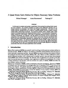
Table 5.4: Convergence results δ = 1e − 2, tolerance = 1e − 8 The behaviour of the error from the coarse level to the finest level is represented in the figure below. The figure gives the visual representation of the behaviour of the error in table(5.4). It depicts a rapid convergence.

Figure 5.3: Behaviour of L2-error The weighting factor of the control has also an impact in the results. The table below shows the effects of the weighting factor on the performance of the method. The results in the table show that the change weighting factor lead the change in the optimal control and the error. The increase in error with increase in the weighting factor means that the weighting factor of the cost functional should be chosen reasonably small. If we take 47

large values of δ the error increases. For this work the value δ = 1e − 2 produce optimal results. The table shows that for large values of weighting factor the discretization error grows. It has been noted in this work that at any grid level the method diverges for the values δ ≤ 1e − 3. The results in the table demonstrates the effect at finest level. w. parameter δ 1e-2 5e-2 1e-1 5e-1 7.5e-1

iterations k 3 3 3 2 2

Control error k k ul kL2 (Ω) k u − ukl kL2 (Ω) 10.36029109 0.00244311 10.36686262 0.00290681 10.36679819 0.00306427 10.36674483 0.00428668 10.36674001 0.00490374

Table 5.5: Changes in δ, l = 5, nodes = 16641, hl = Snapshot of the approximate optimal control at level 4

Figure 5.4: Snapshot of the optimal control at l=4

48

1 128

5.2

Example 2

In this section we focus on the same distributed optimality system in example 1 and solve it with the initial control different from zero. For example, we take u0 = (2π 2 + 1) cos(πx1) cos(πx2). That is taking the exact solution as the initial control. We observe that we achieve the same convergence results and that it converges fast in 2 iterations. The figures in example 1 are the same for this case. We present the results at levels 4 and 5. From the calculations on the finest level we achieve the following results iterations k 1 2

Control tolerance k k k ul kL2 (Ω) k ul − uk+1 kL2 (Ω) l 10.36035509 1.83907065e-5 10.36035560 1.35312409e-13

Table 5.6: l = 4, nodes = 4225, δ = 1e − 2, hl =

iterations k 1 2

Control tolerance k k k ul kL2 (Ω) k ul − uk+1 kL2 (Ω) l 10.36029106 1.15190037e-6 10.36029109 2.0581872e-15

Table 5.7: l = 5, nodes = 16641, δ = 1e − 2, hl =

5.3

error k u − ukl kL2 (Ω) 0.00976765 0.00976709 1 , 64

tolerance = 1e − 8

error k u − ukl kL2 (Ω) 0.002444314 0.002443111 1 , 128

tolerance = 1e − 8

Example 3

In this section we consider the case where the exact solutions are not known. We choose the target state not depending on the exact solutions. We choose the target state as yd = x1 + x2 and the using a zero initial control.

49

Figure 5.5: Desired/Target State at l=4

The behaviour of the control and the stopping criteria on tables(5.8, 5.9, 5.10) from the coarse grid to the finest grid reflect that the method converges to the optimal control. level l 1 2 3 4 5

iterations k 4 3 3 3 3

Control k ukl kL2 (Ω) 2.23636568 2.24634503 2.24879971 2.24941154 2.24946390

Table 5.8: Control, δ = 1e − 2, tolerance = 1e − 8

50

In this case we illustrate the results at levels 4 and 5. The results for all the levels are presented in the tables(5.9) and (5.10). no. of iterations Control tolerance k k k k ul kL2 (Ω) k ul − uk+1 kL2 (Ω) l 1 2.24956732 5.06055475 2 2.249411145 2.680565e-7 3 2.249411154 5.1360268e-15 Table 5.9: l = 4, nodes = 4225, δ = 1e − 2, hl =

1 , 64

tolarence = 1e − 8

The results for the finest level no. of iterations Control error k k 2 k k ul kL (Ω) k ul − uk+1 kL2 (Ω) l 1 2.24960274 5.0607125 2 2.24995638 1.674958e-8 3 2.24946390 2.0000481e-17 Table 5.10: l = 5, nodes = 16641, δ = 1e − 2, hl =

1 , 128

tolerance = 1e − 8

The figure below represents the optimal control for this case. The result was achieved in 5 iterations of the multigrid method,

51

Figure 5.6: Above: Initial Control. Below: Approximate solution for the control at level 4

5.4

Conclusion

In this work we considered the mathematical model of the optimal control problems governed by the elliptic partial differential equations. We have highlighted that the model can be described by the distributed control or boundary control with Neumann or Dirichlet boundary conditions. However, in this work we have given the mathematical treatment to the distributed control model governed by the elliptic partial differential equation with a zero Neumann boundary data. The same mathematical treatment can be applied to control problems the with Dirichlet, non-zero Neumann data. Also the same treatment can be applied to the models where the control is on the boundary, boundary control optimal problems. We described the existence of minimizer of the cost functional which is the control variable. For the distributed control we have shown that the optimal control problem can be expressed as a integral equation where the multigrid method is applied to compute for the optimal control. We have established that multigrid method converges by a factor proportional to the refinement step h between consecutive multigrid iterations. In this work we have used the W-cycle of the multigrid method. We started with an initial guess for initial control, smooth, calculate the defect, restrict, solve exactly on the coarse grid then prolongate and coarse grid correction. For the numerical implementation we use the finite element with piecewise linear elements.

52

We test our method by an example with different cases namely, non-zero initial control, zero initial control and a case where the exact solutions are unknown where the target state is prescribed. We observe that the iteration for the multigrid method decreases rapidly with the fineness of the grids.

53

Bibliography [1] Borzi, A. and Kunisch, K. A Multigrid Scheme for Elliptic Constrained Optimal Control Prpblems, Computational Optimaization and Applications, 31(2005), 309333. [2] Borzi, A . Smoother for Control-and State- constrained Optimal Control Problems, Computational Science, 11(2008), 59-66. [3] Braess, D. Finite Elements, Cambridge University press, 2007. [4] Brenner , C. S and Scott, R. L. The Mathematical Theory of Finite Element Methods, Springer, New York, 2008. [5] Ciarlet, Philippe G. The finite element methods for elliptic problems, North- Holland publishing company, 1978 [6] Hackbusch, W. Fast solution of elliptic control problems, Journal of Optimization Theory and Appli- cation, 31 (1980), 565581. [7] Hackbusch, W. On the fast solving of parabolic boundary control problems, SIAM J. Control and Optim., 17 (1979), pp. 231244. [8] Hackbusch, W. Multi-grid Methods and Applications, Springer-Verlag, New York, 1985. [9] Hackbusch, W. Die schnelle Auflsung der Fredholmschen Integralgleichung zweiter Art, Beitrige Numer. Math 9.(1981), 47-62. [10] Hinze, M.(etal). Modelling and Optimization of PDE-constrained problems, Short Summary of Autumn School 2005, 26.-30. September 2005, Hamburg. [11] Knabner, P. and Angermann, L. Numerical Methods for Elliptic and Parabolic Differential Equations, Springer, Berlin, 2003

54

Eidesstattliche Erkl¨ arung Ich, Kizito Muzhinji, erkl¨are an Eides statt, dass ich die vorliegende Diplomarbeit selbst¨andig und ohne fremde Hilfe verfasst, andere als die angegebenen Quellen und Hilfsmittel nicht benutzt bzw. die w¨ortlich oder sinngem¨aß entnommenen Stellen als solche kenntlich gemacht habe.

Linz, August 2008 Muzhinji Kizito