Multilayer Perceptron Neural Network (MLPs) For ...

World Applied Sciences Journal 5 (5): 546-552, 2008 ISSN 1818-4952 © IDOSI Publications, 2008

Multilayer Perceptron Neural Network (MLPs) For Analyzing the Properties of Jordan Oil Shale 1

2

3

Jamal M. Nazzal, Ibrahim M. El-Emary and Salam A. Najim

1,3

2

Al Ahliyya Amman University, P.O. Box 19328, Amman, Jordan King Abdulaziz University, P.O. Box 18388, Jeddah, King Saudi Arabia

Abstract: In this paper, we introduce the multilayer preceptron neural network and describe how it can be used for function approximation. The back propagation algorithm (including its variants) is the principle procedure for training multilayer perceptrons. Car must be taken when training perceptron network to ensure that they do not over fit the training data and then fail to generalize well in new situations. So the main purpose of this paper lies in studying the effect of changing both the No of hidden layers of MLPs and the No of processing elements that exist in the hidden layers on the analyzed properties of Jordan Oil Shale. After constructing such a MLP and changing the number of hidden layers, we found that with increasing the number of processing elements in the hidden layers. We reach to an optional output results w.r.t the experimental one or the analytical formulated one. This obtained output is completely matched with the main concepts of theoretical visions of ANN. Key words: MLP El-lojjin oil sigmoid perceptron DM-1 Dm-2 •

•

•

•

•

INTRODUCTION

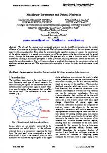
principles. In this paper we want to give a complete description to neural networks and their application in analyzing and studying the properties of Jordan oil shale as a recent technique. At the same time, we would like to investigate the effect of changing the number of processing elements that exist in the hidden layer of the ANN on the forecasted parameters. To check the effectiveness of the described ANN, a comparative study was done between the estimated parameters by ANN and that one that is obtained through experiment or calculated using the formula given in Eg.1. In this paper, we concentrate on the most common neural network architecture called the multilayer perceptron MLPs. For the purpose of this paper, we will look at neural network as function approximators [3]. As shown in Fig. 1, we have some unknown function that we wish to approximate. We want to adjust the parameters of the network so that it will produce the same response as the unknown function, if the same input is applied to both systems. For our application, the unknown function may correspond to a system (oil shale) we are trying to control as a result of analysis, in which case the neural network will be the identified plant model. The unknowing function could also represent the inverse of a system (oil shale) we are trying to control and analyze, in which case the neural network can be used to implement the controller. This paper is organized from six sections. In section two, we describe the

A geochemical analysis of El-Lajjun oil shall in Jordan was carried out [1]. It was found that El-Lajjun oil shale consists of the following group: Organic matter, biogenic calcite and apatite, detrital clay minerals and quartz. The calorific values of 100 samples were determined. The effect of bore depth, calcium carbonate, organic carbon and sulfur content on the calorific values was studied [1]. The results were well correlated by some empirical formula given by [1]: Calorific value=352.44 (CaCo3)-0.066(S) 0.257(Corg)1.143

(1)

With correlation coefficient of 0.983 and with an average standard error of 2.63%. The current resurgence of interest in ANNs is largely due to the emergence of powerful new methods as well as to the availability of computational power suitable fir simulation. The field is particularly exciting today because ANN algorithms and architectures can be implemented in VLSI technology for real time applications [2]. Currently two principal streams can be identified in ANN research. Researches in the first stream are concerned with modeling the brain and thereby explain its cognitive behavior. On the other hand, the primary aim of researches in the second streams is to construct useful computers for real world problems of pattern recognition by drawing these

Corresponding Author: Dr. Jamal M. Nazzal, Al Ahliyya Amman University, P.O. Box 19328, Amman, Jordan

546

World Appl. Sci. J., 5 (5): 546-552, 2008 Unknown Function

-

Input

+ Neural Network

Error

Output

+ Predicted Output

Adaptation

Fig. 1: Neural network as function approximator neuron model. Section three was devoted to Multilayer Perception Architecture. Section five discusses a lot of obtained results. Finally section six presents the results, conclusion and future works done by others. Section four was dedicated to describe the operation of Multilayer Perception Neural Networks. NEURON MODEL The multilayer perception neural network is built up of simple components. In the beginning, we will describe a single input neuron which will then be extended to multiple inputs. Next, we will stack these neurons together to produce layers [4]. Finally, the layers are cascaded together to form the network.

Fig. 2: Single input neuron [4]

Single-input neuron: A single-input neuron is shown in Fig. 2. The scalar input p is multiplied by the scalar weight W to form Wp, one of the terms that is sent to the summer. The other input, 1, is multiplied by a bias b and then passed to the summer. The summer output n often referred to as the net input, goes into a transfer function f which produces the scalar neuron output a (sometimes "activation function" is used rather than transfer function and offset rather than bias). From Fig. 2, both w and b are both adjustable scalar parameters of the neuron. Typically the transfer function is chosen by the designer and then the parameters w and b will be adjusted by some learning rule so that the neuron input/output relationship meet some specific goal. The transfer function in Fig. 2 may be a linear or nonlinear function of n. A particular transfer function is chosen to satisfy some specification of the problem that the neuron is attempting to solve. One of the most commonly used functions is the log-sigmoid transfer function, which is shown in Fig. 3 [4]. This transfer function takes the input (which may have any value between plus and minus infinity) and

Fig. 3: Log-sigmiod transfer function squashes the output into the range 0 to 1 according to the expression: a=

1 1 + e− n

(2)

The log-sigmoid transfer function is commonly used in multi-layer networks that are trained using the back propagation algorithm. Multiple-input neuron: Typically, a neuron has more than one input. A neuron with R inputs is shown in Fig. 4. The individual inputs p 1 , p 2 ,……, p g are each 547

World Appl. Sci. J., 5 (5): 546-552, 2008

dimensions of p are displayed below the variable as Rx1, indicating that the input is a single vector of R elements. These inputs go to the weight matrix W, which has R columns but only one row in this single neuron case. A constant 1 enters the neuron as an input and is multiplied by a scalar bias b. The net input to the transfer function f is n, which is the sum of the bias b and the product Wp. The neuron's output is a scalar in this case. If there exit more than one neuron, the network output would be a vector. Fig. 4: Multiple-input neuron

MULTILAYER PERCEPTRON NETWORK ARCHITECTURES Commonly one neuron, even with many inputs, may not be sufficient. We might need five or ten, operating parallel, in what we will call a “layer". This concept of a layer is discussed below. A layer of neurons: A single-layer network of S is shown in Fig. 6. Note that each of the R inputs is connected to each of the neurons and that the weight matrix now has s rows. The layer includes the weight matrix, the summers, the bias vector b, the transfer function boxes and the output vector a. Each element of the input vector p is connected to each neuron through the weight matrix W. Each neuron has a bias b i , a summer, a transfer function f and an output a i . Taken together, the outputs form the output vector a. It is common for the number of inputs to a layer to be different from the number of neurons (i.e. R≠S). The input vector elements enter the network through the weig ht matrix W:

Fig. 5: Neuron with R inputs, abbreviated notations weighted by corresponding elements W 1,1 W 1,2 ,….W 1,R of the weight matrix W. The neuron has a bias b, which is summed with the weight inputs to form the net input n: = n W1,1 p1 + W1,2 p 2 + ... + W1,R p R + b

(3)

This expression can be written in matrix form as: = n Wp + b

(4)

Where the matrix W for the single neuron case has only one row. Now the neuron output can be written as: = a f(Wp + b)

(5)

A particular convention in assigning the indices of the elements of the weight matrix has been adopted [4]. The first index indicates the particular neuron destination for the weight. The second index indicates the source of the signal fed to the neuron. Thus, the indices in W 1,2 say that this weight represents the connection to the first (and only) neuron from the second source [4]. A multiple-input neuron using abbreviated notation is shown in Fig. 5. As shown in Fig. 5, the input vector p is represented by the solid vertical bar at left. The

Fig. 6: Layer of S neurons 548

World Appl. Sci. J., 5 (5): 546-552, 2008

weight matrix W, its own bias vector b, a net input vector n and an output vector a. Some additional notation should be introduced to distinguish between these layers. Superscripts are used to identify these layers. The number of the layer as a superscript is appended to the names for each of these variables. Thus, the weight matrix for the second layer is written as W 2 . This notation is used in the three-layer network shown in Fig. 8. As shown in Fig. 8, there are R inputs, S 1 neurons in the first layer, S 2 neurons in the second layer, etc. The output of layers one and two are the inputs for layers two and three. Thus layer 2 can be viewed as a one-layer network with R=S1 inputs, S= S 2 neurons and an S 1 *S 2 weight matrix W2 . The input to layer 2 is a 1 and the output is a 2 . A layer whose output is the network output is called an output layer. The other layers are called hidden layers. The network shown in Fig. 8 has an output layer (layer3) and two hidden layers (layers 1 and 2)

Fig. 7: Layer of S neurons, abbreviated notation W1,1

...

W1,R

W=    Ws,1 ... WS , R

(6)

The row indices of the elements of matrix W indicate the destination neuron associated with that weight, while the column indices indicate the source of the input for that weight. Thus, the indices in W3,2 say that this weight represents the connection to the third neuron from the second source. The S-neuron, R-input, one-layer network also can be drawn in abbreviated notation as shown in Fig. 7. Here again, the symbols below the variables tell that for this layer, p is a vector of length R, W is an S*R matrix and a and b are vectors of length S. As defined previously, the layer includes the weight matrix, the summation and multiplication operations, the bias vector b, the transfer function boxes and the output vector.

STRUCTURE AND OPERATION OF MULTILAYER PERCEPTRON NEURAL NETWORK (MLP) MLP neural networks consist if units arranged in layers [5]. Each layer is composed of nodes and in the fully connected network considered here each node connects to every node in subsequent layers. Each MLP is composed of a minimum of three layers consisting of an input layer, one or more hidden layers and an output layer. The input layer distributes the inputs to subsequent layers. Input nodes have liner activation functions and no thresholds. Each hidden unit node and each output node have thresholds associated with them in addition to the weights. The hidden unit nodes have nonlinear activation functions and the outputs have linear activation functions. Hence, each signal feeding into anode in a subsequent layer has the original input multiplied by a weight with a threshold added and then

Multiple layers of neurons: Now consider a network with several layers which has been implemented in this paper for the purpose of analyzing Jordan oil shale properties. In this network each layer has its own

Fig. 8: Three layer network 549

World Appl. Sci. J., 5 (5): 546-552, 2008

Fig. 9: Typical three layer multilayer perceptron neural network is passed through an activation function that may be linear or nonlinear (hidden units). A typical three layer network is shown in Fig. 9. Only three layer MLPs will be considered in this work since these networks have been shown to appro ximate any continuous function [6-8]. For the actual three layers MLP, all of the inputs are also connected directly to all of the outputs [5]. The training data consist of a set NV training patterns (x p ,t p ) where P represents the pattern number. In Fig. 9, XP corresponds to the N-dimensional input vector of the Pth training pattern and YP corresponds to the M-dimensional output vector from the trained network for the Pth pattern. For ease of notation and analysis, threshold on hidden units and output unit s are handled by assigning the value of one to an augmented vector component denoted by Xp (N+1). The output and input units have linear activations. The input to the Jth hidden unit, net P (j) is expressed [5] as: = net p (j)

∑

N +1 k =1

Whi (j,k)Xp (k) 1 ≤ j ≤ N h

The overall performance of the MLP is measured by the mean square error (MSE) expressed by : = E

1 Nv 1 Nv M = ∑ Ep N ∑ ∑i 1[t p (i) − y p(i)]2 = p 1= N =p 1

Where: = Ep

∑

M i= 0

[t p (i) − yp (i)]2

= Ei

1 M ∑ [t p (i) − y p (i)]2 N v p =1

(7)

1+ e

− n e tp( j )

CONCLUSION

(9)

In (7) and (8), the N input units are represented by the index K and Whi (J,K) denotes the weight connecting the Kth input unit to the Jth hidden unit.

(13)

In (13), Woi (i,k) represents the weight from the input nodes to the output nodes and Woh (i,j) represents the weight from the hidden nodes to the output nodes.

(8)

The nonlinear activation is typically chosen to be the sigmoid function f(net p (j)) =

(12)

with the i th output for the Pth training pattern expressed by: h

1

(11)

Ep Corresponds to the error for the Pth pattern and t p is the desired output for the Pth pattern. This is also allows the calculation of the napping error for the i th output unit to be expressed by:

N +1 N With the output activation for the Pth training pattern, = Yp( i ) ∑ k 1= Woi (i,k)X p (k) + ∑ j 1 Woi (i,j).O p (j) = Op (j), being expressed by:

O p( j) = f(net p( j))

(10)

550

When investigators design neural networks for the application presented in this paper, there are many ways used to investigate the effects of network structure which refers to the specification of network size (i.e. number of hidden units) when the number of inputs and

World Appl. Sci. J., 5 (5): 546-552, 2008

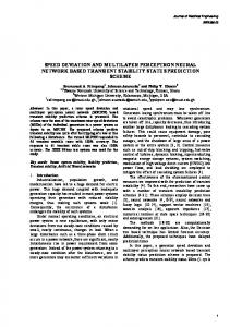
Fig. 10: CaCo3 versus gross calorific value

Fig. 11: Corg versus gross calorific value

Fig. 12: S versus gross calorific value 551

World Appl. Sci. J., 5 (5): 546-552, 2008 Table 1: Results summary Performance

MLP ANN 3:10:1

MLP ANN 3:20:1

MLP ANN 3:10:10:1

MLP ANN 3:20:10:1

MSE

120517.0498

94695.29502

105564.1689

96255.51725

NMSE

0.019660591

0.01544815

0.017221248

0.015702678

MAE

239.4225634

213.4408001

220.7435148

209.1266576

Min Abs Error

7.123826454

1.171097513

8.106955387

1.71756787

Max Abs Error

1427.779547

1184.631573

1375.296117

1307.388839

r

0.990186314

0.992293629

0.991392243

0.992167131

REFERENCES

outputs are fixed (5) which in turn affects on the o/p predicted parameters. A well organized one maybe based on designing a set of different size networks in an ordinary fashion, each with one or more hidden units than the previous one. This approach can be designated as design methodology one (DM -1). Alternatively, the second one is based on designing different size networks in no particular order. This approach can be designated as design methodology two (DM-2). These two design approaches are significantly different and the approach chosen often is based on the goals set for the network design and the associated performance. In general, the more thorough approach often used for DM-l may take more time to develop the selected network since we may be interested in trying to achieve a trade-off between network performance and network size. However, the DM-1 approach used in this work may produce a superior design since the design can be pursued until we will be satisfied that future increases in network size produces diminishing returns in terms of decreasing training time or testing errors. When we design MLP network to analyze the properties of Jordan oil shale, we reach to the following facts: MLP with a lot of hidden layers (3) performs more better than with one or two hidden layer specially regarding the output performance parameters. Also, when we compare between the o/p of MLP and the mathematical formula, we found that our o/p performance parameter are best suited with the experimental. As a future work, we recommend to use hybrid approaches, which are a combination of ANN with other techniques like expert systems, Fuzzy logic and Genetic Algorithm (GA) to make such analysis of Jordan oil Shale properties.

1.

2.

3. 4. 5.

6. 7.

8.

552

Anabtawi, M.Z. and jamal M. Nazzal, 1994. Effect of composition of el-lajjun oil shale on its calorific value. Journal of Testing and Evaluation, pp: 175-178. Nitin Malik, 2005. Artificial Neural Networks and their Applications. National conference on Unear thing Technological Developments & their transfer for serving Masses, GLA ITM, Mathura, Mathura, India. Martin, T. Hagan and Howard B. Demuth, Neural Networks for control, www.uldaho.edu Haykin, S., 1999. Neural Networks: A Comprehensive Foundation, 2nd Edn., New Jersey: Prentice-Hall. Walter, H. Delashmit and Michael T. Manry, 2005. Recent Developments in Multilayer Perceptron Neural Networks. Proceedings of the 7th Annual Memphis Area Engineering and Science Conference, MAESC 2005. Hornik, K., M. Stinchcombe and H., White, 1989. Multilayer feed forward Networks are Universal Approximators, Neural Networks, 2 (5): 35g, 366. Hornik, K., M. Stinchombe and H. White, 1990. Universal Approximation of an unknown Mapping and its Derivatives Using Multilayer Feed forward Networks. Neural Networks, 3 (5): 551-560. Cybenko, G., 1989. Approximation by superposition of a sigmoidal function. Mathematics of control, Signal and Systems, 2 (4): 303-314.