Key words: phase-change memory (PCM), multilevel cell (MLC), non-volatile memory. 1. ... sub-threshold conduction regime in conjunction with the trap-limited ...
B02
E*PCOS2009
Multilevel Phase-Change Memory Modeling and Experimental Characterization A. Pantazi, A. Sebastian, N. Papandreou, M. J. Breitwisch*, C. Lam*, H. Pozidis, E. Eleftheriou IBM Research - Zurich, CH-8803 Rüschlikon, Switzerland *IBM Research - T.J. Watson Research Center, 1101 Kitchawan Road, Yorktown Heights, NY 10598 ABSTRACT Phase-change memory (PCM) has emerged in recent years as the most promising technology for non-volatile memory due to its very high throughput performance and read/write endurance as well as future scalability. Multilevel functionality is crucial for increasing the capacity and thus enhancing the cost per GByte competitiveness of the PCM technology. However, storage of multiple resistance levels in a PCM cell is a challenging problem; issues like process variability, as well as intra-cell and inter-cell material parameter variations give rise to deviations in the achieved resistance levels from their intended target values. Therefore, iterative programming schemes are required employing multiple write-verify steps until the desired resistance level is reached. A thorough understanding of the characteristics of the PCM cells is essential for the design of an effective programming algorithm. In this paper, we present a systems-based model that captures the essential behavior of the PCM cell. In particular, the model captures the interplay between the electrical, thermal and phase-change parts of the system. Experimental results at various intermediate cell states were utilized to characterize the PCM cell behavior and fit the model parameters. The systemsbased model of the PCM cell is a powerful tool for the design of efficient iterative multilevel programming algorithms. Finally, schemes that adaptively control parameters of the programming pulse in an iterative manner are presented, and experimental results on PCM cells demonstrating the efficacy of the presented programming schemes in achieving multilevel functionality are discussed. Key words: phase-change memory (PCM), multilevel cell (MLC), non-volatile memory 1. INTRODUCTION Phase-change memory is an emerging non-volatile solid-state memory technology relying on the reversible, thermally-assisted phase transitions of chalcogenide materials. Besides the superior write speed, PCM offers in addition multilevel cell (MLC) functionality by exploiting the wide resistance range between the crystalline (SET) and amorphous (RESET) states. During device fabrication, process variability can create dimensional and material nonuniformities across an array of PCM cells that give rise to variations of the achieved resistance level in a single-pulse programming approach. The common solution is to employ iterative programming schemes for MLC programming [1], [2]. Characterization and modeling of the PCM cell is essential for the design of effective MLC programming algorithms. In this paper, we present an efficient cell characterization method based on simple electrical measurements and a systems-based modeling approach that captures the essential behavior of the PCM cell. Experimental studies of the sub-threshold conduction regime in conjunction with the trap-limited transport model of Ielmini-Zhang [3] provide useful cell parameters, such as the effective thickness of the amorphous part, and form the basis of the electrical part of the PCM model. The thermal and phase-change parts of the model are also described and a comparison of simulated and experimental data is presented. The systems-based model is a powerful tool for the development of efficient MLC programming schemes. In the multilevel programming approach presented in this work the PCM cell is viewed as an operator, mapping an input signal, i.e., an attribute of the programming pulse, to the output, i.e., the resulting resistance level of the memory cell. MLC programming schemes based on different operators are presented and experimental results demonstrate their convergence to various target resistance levels.
34
B02
2. CELL CHARACTERIZATION AND MODELING The memory cells studied in this work are of the commonly used “mushroom” type, where a doped Ge2Sb2Te5 (GST) phase change material is sandwiched between TiN electrodes. The thickness of the phase change material is approx. 100 nm and the bottom electrode has a diameter of approx. 40 nm. The phase change element (PCE), comprising the GST material and the electrodes, is connected in series with an nMOSFET access device based on 180 nm CMOS technology [4]. A 10x10 array test structure of memory cells is connected to the experimental setup as shown in Fig. 1. A pulse pattern generator is used to provide the word-line (WL) programming pulse, while a custom-made hardware board is utilized for the bit-line (BL) programming voltage and for high precision current measurements through an off-chip load resistance RL. Switching between the memory cells of the 10x10 array is provided by a programmable switch system.
Fig. 1 Experimental set-up.
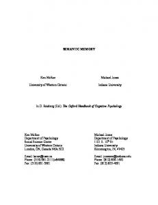
Fig. 2 Block diagram of PCM model.
For a complete description of the characteristics and the MLC functionality of the phase-change memory the PCM cells were experimentally characterized and a systems-based model has been developed. The model of the PCE, the block diagram of which is shown in Fig. 2, captures the interplay between the electrical, thermal and phase-change parts of the system. The PCM cell model includes the characteristics of the transistor that has been independently characterized. Fig. 3 shows the experimentally measured current at the drain ( I d ) versus the gate voltage ( Vg ) and the drain voltage ( Vd ) of the access transistor.
Fig. 3 FET access device characteristics.
Fig. 4 Cell resistance corresponding to programming pulses of varying amplitude applied at the WL.
The experimental procedure for characterizing the behavior of the PCM cells at various intermediate cell states includes three steps for each resistance state. In the first step, the memory cell is programmed in the SET (lowest resistance) state. In the second step, it is programmed in an intermediate resistance level. In the third and final step, the I-V characteristic of the cell being at that resistance level is obtained. Programming of the cell is achieved by operating the transistor as a current source, i.e. the BL is kept constant at a voltage of 3 V and the current through the
35
B02
cell is controlled by varying the WL voltage. To achieve various resistance levels, a rectangular voltage pulse is applied to the WL with amplitude ranging from 0 to 4 V in steps of 0.1 V. The rectangular pulse has a leading edge (LE) of 50 ns, trailing edge (TE) of 10 ns and a pulse width of 200 ns in all cases. Fig. 4 shows the resistance of the cell measured at low voltage Vread = 0.3 V as a function of the programming voltage applied at the WL. As the cell is initially in the SET state, corresponding to the minimum thickness of the amorphous material, application of lowamplitude pulses does not change the state of the cell. As the voltage (and equivalently the current) increases, the local temperature exceeds the melting point and results in the formation of new amorphous material, therefore the resistance of the cell increases.
Fig. 5 I-V characteristics of the PCM cell at the RESET and SET states.
Fig. 6 Subthreshold I-V curves. Marks indicate measured data, whereas lines are model fits to the data.
Having programmed the cell in a particular resistance level, I-V measurements in both the subthreshold conduction regime as well as in the dynamic programming regime are collected. Fig. 5 shows the characteristic I-V of the memory cell in the SET state and in the RESET (high resistance) state. Starting from the RESET state, as the voltage increases a critical threshold voltage, Vth , is exceeded and a characteristic resistance drop is observed. At this point the cell switches rapidly from the so-called “OFF” state into the dynamic “ON” state. In the case of a SET state, the cell exhibits a low electrical resistance and as the voltage increases the I-V curve eventually coincides with that of the RESET state. In the specific experimental data, the characteristic I-V of the access transistor dominates because the resistance of the PCE in the “ON” regime is very low and the Vg voltage was set to 1 V (see Fig. 3). Only after the cell has switched to the “ON” state, a phase-change transition is possible via Joule heating by the current that flows through the cell. Therefore, cell programming can be achieved in the “ON” state, whereas cell read-out is performed in the “OFF” state to avoid disturbance of the phase of the material. In the subthreshold regime the I-V curves exhibit a linear behavior for small voltages, followed by an exponential one at higher voltages [3]. This behavior can be described by expressing the current at the subthreshold regime by the following formula:
I=
1 sinh (Va β ) R0 β
(1)
where R0 is the low-field resistance, Va is the applied voltage and β describes the subthreshold slope, which is defined as
β=
qΔz kT 2ua
36
(2)
B02
where q is the elementary charge, k is the Boltzmann constant and T is the temperature [3]. The slope β is proportional to Δz u a , that is, the average inter-trap distance normalized to the amorphous material thickness. By fitting the model of (1) to the subthreshold I-V measurements, we can extract the values of β and R0 for the various cell resistance levels between the SET and RESET states. Fig. 6 shows the results of the fit. Very good agreement between measurements and model is obtained, verifying once more the theory of trap-limited transport in the subthreshold regime, proposed in [3]. Less accurate fitting is achieved for low cell resistance states, where alternate conduction mechanisms become significant and the accuracy of the trap-limited transport model deteriorates. Using the estimated values of β and R0 for the various resistance levels and a methodology similar to the one presented in [5], the amorphous fraction can be estimated. Specifically, the estimation procedure is as follows: 1) First obtain an estimate of the maximum thickness of the amorphous material in the RESET state using the equation ua = Vth Fth , where Fth is the critical switching field [3]. For Vth = 1.35 V, as extracted from Fig. 5, and Fth = 0.44 MVcm-1, a typical literature value, we get a maximum u a = 30 nm. 2) Based on the above estimate of u a , the estimated value of β in the RESET state and the equation (2) the material parameter Δz is extracted. 3) Keeping the material parameter Δz fixed, an estimate of the effective amorphous thickness u a for the different resistance levels corresponding to the I-Vs of Fig. 6 is extracted using equation (2). Based on the above experimental characterization of the PCM cell behavior, an electrical model that accounts for the intermediate resistance levels can be defined. The amorphous fraction parameter Ca is defined as Ca = u a t gst , where t gst is the total thickness of the phase-change material within the PCE. Based on the estimated amorphous thickness in the SET and RESET states the minimum and maximum achievable values of Ca , i.e., Ca min and Ca max can be derived. In practice, and as it was also verified experimentally, u a does not reach the value of t gst as the low thermal resistance of the top electrode prohibits the temperature from reaching the melting temperature in the area close to the top electrode. Similar to Ca , the minimum and maximum values of β and R0 can be defined. Therefore, based on the experimental data, the electrical part of the model shown in Fig. 2 can be described using equation (1), where β −1 and R0 are linear functions of the amorphous fraction Ca and are given by the following equations
⎛R − R0 min R0 (C a ) = R 0 min + ⎜⎜ 0 max ⎝ C a max − C a min
⎞ ⎟(C a − C a min ) ⎟ ⎠
⎛ β −1 max − β −1 min β −1 (C a ) = β −1 min + ⎜⎜ ⎝ C a max − C a min
⎞ ⎟(C a − C a min ) ⎟ ⎠
(3)
(4)
Fig. 7 shows the model response compared with the experimentally estimated data for the low-field resistance of the cell. As shown in the figure the proposed model accurately captures the behavior of the PCM cell in the subthreshold regime. For modeling the threshold switching regime, a constant threshold switching current I t is assumed [6]. The value of I t is set at 3.5 μA based on the experimental data shown in Fig. 5. The resistance of the cell after threshold switching is assumed to be small and independent of the amorphous fraction Ca .
37
B02
Fig. 7 Low-field resistance vs amorphous fraction.
Fig. 8 Measured and simulated response.
The thermal system model is similar to that presented in [6]. However, to capture the significant difference in the width of the bottom and top electrodes, the thermal resistances and the subsequent temperature distribution is evaluated slightly differently. For a bottom electrode radius Rb and top electrode radius Rt the thermal resistances of the amorphous and crystalline regions are given by
⎤ ⎥ , respectively, where ρ a and ρ c are the thermal ⎥⎦ Rb t gst resistivities of amorphous and crystalline GST, respectively, and x = . Rt − Rb
Rta =
ρa x2 πRb 2
⎡1 1 ⎤ and ρ x2 Rtc = c 2 ⎥ ⎢ − πRb ⎣ x x + ua ⎦
⎡ 1 1 ⎢ − ⎢⎣ x + ua x + t gst
The crystallization and amorphization dynamics are modeled in a similar manner as in [6]. The crystallization rate is calculated based on the nucleation-growth model and the melting rate is calculated using the latent heat. Finally, the full systems-based model is derived by interconnecting the electrical, thermal and phase-change subsystems as shown in Fig. 2. Fig. 8 shows the comparison of the experimental data with the response of the model for the low-field cell resistance as a function of the programming voltage applied at the WL. There is good agreement between the two given that the model is very simplistic compared to elaborate 3-D simulation models. Similarly we can obtain the cell resistance as a function of the amplitude of the voltage pulses applied at the BL. The PCM cell can be viewed as an operator mapping the parameter of the programming pulse to the resulting resistance value that is achieved. The system level model helps generate and understand these operators. These operators are essential for multilevel programming and in particular for the design of iterative programming schemes for multilevel recording. This will be addressed in the next section.
3. MULTILEVEL CELL PROGRAMMING Reliable multilevel functionality is crucial for cost and performance competitiveness of the PCM technology. However, in multilevel storage, issues like process variability give rise to deviations of the achieved resistance levels from their intended values. For example, Fig. 9 shows the programming curves of various cells from the 10x10 array that can be obtained with a single 200 ns programming pulse of varying amplitude at the WL. As shown in the figure, even though the programming curves exhibit similar overall behavior, there are variations between them that would result in broad cell resistance distributions if a single step programming approach were utilized. Therefore, an iterative programming scheme is required, with multiple write-verify steps until the desired resistance level is reached [1], [2].
38
B02
Fig. 9 Programming curve for various cells.
Fig. 10 Block diagram of the control scheme.
In the multilevel programming approach, presented in this work, the PCM cell is viewed as an operator mapping an input signal to the output, i.e. the resulting resistance level. As there are several input signals that can be varied in order to modify the resistance of the memory cell, different operators are defined and utilized for multilevel programming. In this paper the following operators are explored: 1) an operator mapping the amplitude of the WL programming pulse to the cell resistance, 2) an operator mapping the amplitude of the BL programming pulse to the cell resistance, and 3) an operator mapping the duration of the trailing edge of the WL programming pulse to the cell resistance. After the operator is defined, a control structure that generally consists of a feedback and a feedforward part is utilized for MLC programming. The structure of the control scheme is illustrated in Fig. 10. The PCM cell is described by the operator which maps an input V (k ) to the resulting cell resistance R(k ) . The controller consists of a feedback part that takes as an input the resistance error with respect to a reference resistance and a feedforward term that provides faster response to the control loop. As a continuous measure of the resistance is not available, a read operation is performed after each write cycle to reliably measure the cell resistance. Different feedback controllers can be designed, ranging from PID to more complicated algorithms, but a simple integral controller is utilized in this work. Integral control is particularly suitable for systems which are susceptible to significant model variation. Control using the first operator i.e., the amplitude of the gate voltage, amounts to controlling the current that flows through the cell as the transistor is biased at a high drain voltage thus operating as a current source. Fig. 11 shows the programming curves mapping the amplitude of the WL pulse to the resistance of the cell measured at low voltage. Two programming curves are shown where either the RESET or the SET states are considered as the initial state of the cell at each programming point. Two operating regimes are possible; the left slope, obtained by progressively crystallizing the phase-change material with increasing amplitude pulses and the right slope, where application of each programming pulse is melting the material. The left slope is typically steeper and uni-directional, that is, starting from a specific point only decreasing the resistance is possible by increasing the pulse amplitude. The right slope is bidirectional, as shown in Fig. 11 by the overlapping of the curves starting from RESET or SET initial states, but higher amplitude pulses are required to operate in this regime. From a control point of view, it is simpler to operate in the right slope since overshooting or undershooting the target resistance can be compensated with decreased or increased amplitude pulses, respectively. Fig. 12 shows two sets of intermediate resistance level programming experiments using this operator and the right programming slope. The target resistances were set to 2 MΩ and 500 KΩ. Several experiments were performed and, as shown in Fig. 12, the algorithm has converged to the target resistance within a few iterations. Also shown in Fig. 12 is the bi-directional flexibility of the right slope in the case of overshooting/ undershooting the target resistance. For simplicity, the feedforward term was chosen to be a constant corresponding to the middle of the right slope. A multiplicative gain, as shown in Fig. 10, may be a more appropriate selection for multilevel experiments.
39
B02
Fig. 11 Cell resistance corresponding to programming pulses of varying amplitude applied at the WL.
Fig. 12 Experimental results showing convergence to two intermediate resistance levels.
Programming by varying the WL voltage may have limitations on the chip level since simultaneous programming of multiple cells in the same array may not be possible. Fig. 13 shows another operator that can be used for programming, in particular the programming curve mapping the amplitude of the voltage pulse at the BL to the resistance of the cell, measured at low read voltage. The disadvantage of this operator is that some operating regions are not accessible, for example, for a given cell state the amplitude of the BL voltage must be greater than the Vth at that state in order to enable threshold switching and subsequent programming of the cell. The programming curve for this operator, shown in Fig. 13, starts from the SET state at each programming point and is compared with a similar curve without SET initialization at each point. This operator is also bi-directional as melting occurs at each programming step. Fig. 14 shows similar multilevel programming experiments using this operator, in which convergence is again achieved after a few iterations.
Fig. 13 Cell resistance corresponding to programming pulses of varying amplitude applied at the BL.
Fig. 14 Experimental results showing convergence to two intermediate resistance levels
In contrast to varying the amplitude of a rectangular programming pulse, a third operator can be defined that maps the duration of the trailing edge of the WL programming pulse to the cell resistance and is characterized by the programming curve of Fig. 15. This operator is also bi-directional as the amplitude of the programming pulse is chosen so as to enable melting and the different levels of crystallization are achieved by varying the duration of the trailing edge of the pulse. Fig. 15 shows that the curves both with a RESET at each step and without RESET at each step are matching, as each programming pulse enables melting of the cell at each point. The same set of multilevel
40
B02
experiments is also shown, demonstrating the programming efficacy of the operator based on the trailing edge of the WL voltage pulse.
Fig. 15 Cell resistance corresponding to programming Fig. 16 Experimental results showing convergence to pulses of varying trailing edge duration applied at the WL. two intermediate resistance levels Using the multilevel programming approach in which the PCM cell is viewed as an operator mapping an input signal to the output resistance level, different operators can be compared in terms of reliability, number of iterations, required power etc. The selection of the optimal operator may depend on a number of factors and requires statistical characterization over a large number of cells and resistance levels.
4. CONCLUSIONS A systems-based model for the PCM cell that captures the interplay between the electrical, thermal and phase-change sub-systems was presented. Multilevel programming approaches that utilize different ways of mapping input signals to appropriate resistance levels were studied and compared and experimental results demonstrating the efficacy of each scheme were shown.
REFERENCES 1. T. Nirschl, et. al., “Write Strategies for 2 and 4-bit Multi-Level Phase-Change Memory”, IEDM Tech. Dig., pp. 461-464, 2007. 2. F. Bedeschi, et. al.,“A Bipolar-Selected Phase Change Memory Featuring Multi-Level Cell Storage”, IEEE JSSC, v.44, pp. 217-227, 2009. 3. D. Ielmini and Y. Zhang, “Analytical model for subthreshold conduction and threshold switching in chalcogenidebased memory devices”, J. Appl. Phys. 102 (2007) 054517. 4. B. Rajendran et al., “Dynamic resistance – a metric for variability characterization of phase-change memory,” IEEE Electron Device Lett. 30 (2009) 126. 5. N. Papandreou et al., “Estimation of amorphous fraction in multilevel phase change memory cells”, to appear in ESSDERC 2009. 6. K. Sonoda et al., “A compact model of phase-change memory based on rate equations of crystallization and amorphization”, IEEE Trans. Electron Devices 55 (2008) 1672.
41