Multiperiod Portfolio Selection and Bayesian Dynamic

Multiperiod Portfolio Selection and Bayesian Dynamic Models Techniques inspired by Bayesian statistics provide an elegant solution to the classic investment problem of optimally planning a sequence of trades in the presence of transaction costs, according to Petter Kolm1 and Gordon Ritter1 .

Bayesian statistics. Intuition is most valuable when it is also useful, however, and perhaps the best feature of our framework is that intuition leads to a straightforward algorithm for solving the problem. This algorithm applies to the realistic case when market impact is nonlinear and overall trading cost may not even be differentiable, and with real-world portfolio constraints. We plan to provide more technical details and numerical examples in a companion paper.

Planning a sequence of trades extending into the future is a very common problem in finance. All trading is costly, and the need for intertemporal optimization is more acute when trading costs are considered. The total cost due to market impact is known to be superlinear as a function of the trade size (Almgren et al. (2005) measured an exponent of about 0.6 for impact itself, hence 1.6 for total cost), implying that a large order may be more efficiently executed as a sequence of small orders. Indeed, optimal liquidation paths had already been studied by Almgren and Chriss (1999) under an idealized linear impact model, leading to quadratic total cost. A similar, but more complex problem is faced by the discretionary trader, who can set the time horizon and who can wait to deploy an alpha strategy until there is a trading path with favorable expected utility. Further, the drivers of demand for trading may differ vastly at different horizons. Disagreement among alpha models defined at various horizons is, in fact, commonplace in quantitative trading. Gârleanu and Pedersen (2013) studied the multiperiod quantitative-trading problem under the somewhat restrictive assumptions that the alpha models follow mean-reverting dynamics and that the only source of trading frictions are purely linear market impacts (leading to purely quadratic impact-related trading costs). A third problem, related to the first two, is the practicality of hedging derivative contracts when trading cost of dynamic offsetting replicating portfolios is taken into account. This problem is routinely faced by the office of the CIO at an investment bank, who must balance risk with the cost of trading a large hedging position. In this paper we present a general framework which encompasses all of these types of problems, and which establishes an intuitively appealing link to the theory of 1 Courant

Intuition and a Probabilistic View We now place ourselves into the position of a rational agent planning a sequence of trades beginning presently and extending into the future. Specifically, a trading plan for the agent is modeled as a specific portfolio sequence x = (x1 , x2 , . . . , xT ), where xt is the portfolio the agent plans to hold at time t in the future. If rt+1 is the vector of asset returns over [t, t + 1], then the trading profit (ie. difference between initial and final wealth) associated to the trading plan x is given by X π(x) = [xt · rt+1 − ct (xt−1 , xt )] (1) t

where ct (xt−1 , xt ) is the total cost (including but not limited to market impact, spread pay, borrow costs, ticket charges, financing, etc.) associated with holding portfolio xt−1 at time t − 1 and ending up with xt at time t. Trading profit π(x) is a random variable, since many of its components are future quantities unknowable at time t = 0. The distribution of π(x) need not be normal, and we do not assume normality in this paper. However, a number of important calculations are only tractable if we assume that the investor’s utility function can be approximated by the first two terms in its Taylor series. Thus the problem we treat initially is that of maximizing u(x), where u(x) := E[π(x)] − (γ/2)V[π(x)]

Institute of Mathematical Sciences, New York University, 251 Mercer St, New York, NY 10012

February 11, 2015

1

(2)

Just after Intuition 1 below, we discuss how our framework can be applied to more general problems which transcend (2). We will often refer to a planned portfolio sequence x = (x1 , x2 , . . . , xT ) simply as a “path.” Similarly we sometimes refer to (2) as the “utility of the path x,” while remembering the more complex link to utility theory noted above. Our task, in this simpler language, is to find the maximum-utility path x∗ = argmaxx u(x). Combining (1) with (2), and defining αt := E[rt+1 ] and Σt := V[rt+1 ], one has i Xh γ > x Σ x − c (x , x ) (3) u(x) = x> α − t t t t−1 t t t 2 t t

in the original Black-Litterman model, the two-moment approximation to utility is exact, and one simply replaces αt and Σt with the appropriate quantities. In practice, investors’ utility functions may depend on higher moments (skewness, kurtosis) or partial moments of the distribution of final wealth (Zakamouline and Koekebakker, 2009). Optimal portfolio selection in this case is a hard problem even without transaction costs, as the objective function need not be convex. Suppose, however, that an investor with such a utility function has decided on the trading path y = (yt ) to follow in an ideal world without trading costs. Presumably this has been accomplished via solving a difficult four-moment or mean-CVaR optimization problem. Once y has been determined, we may proceed with maximization of (6) for the purpose of tracking y in a cost-efficient manner. As we shall see, the quadratic distance function bγΣt in (6) may be replaced with any smooth, convex function of its arguments and the optimization technology we discuss later will still apply. For our next piece of intuition, consider the random process model for x = (x1 , x2 , . . . , xT ) given by Z 1 (7) p(x) = exp(κ u(x)), Z := exp(u(κ x))dx Z

Neglecting terms that do not depend on x, the first two terms of (3) are (up to a sign) equivalent to bγΣt (xt , yt ) :=

1 (yt − xt )> γΣt (yt − xt ) 2

(4)

where yt := (γΣt )−1 αt .

(5)

The latter is a classic mean-variance portfolio, which is well-known to be the solution to a myopic problem without costs or constraints, and bγΣt measures variance of the tracking error. Then up to x-independent terms, for an arbitrary constant κ > 0. In realistic models, Z is always finite. The constant κ is analogous to the inverse X u(x) = − [bγΣt (xt , yt ) + ct (xt−1 , xt )] (6) temperature in statistical physics. t Optimizing expected utility is then equivalent to predicting the most likely action of a randomly-acting agent In any multiperiod optimization problem with transwhose actions are probability-weighted by (7). We will action costs, one can always ask what the solution would refer to this agent as the random trader. be in an ideal world without transaction costs, or equivIf u(x) is of the form (6) for any ideal sequence yt , alently, in the limit as costs tend to zero. We call this then p(x) naturally has a product form: solution the ideal sequence, and always denote it by yt . Y Intuition 1. Multiperiod portfolio optimization is mathep(x) = p(yt | xt )p(xt | xt−1 ) (8) matically equivalent to optimally tracking a sequence yt , t called the ideal sequence, which is the portfolio sequence where that would be optimal in a transaction-cost free world. The general guiding principle expressed as Intuition 1 extends beyond the case in which the ideal sequence is (γΣt )−1 αt , and indeed, beyond the case in which yt has a clean derivation from a utility function. For computing optimal liquidation paths in the spirit of Almgren and Chriss (1999), the ideal sequence is clearly yt = 0 for all t. For hedging exposure to derivatives, yt should be our expectation of the offsetting replicating portfolio at all future times until expiration. Tracking the portfolios of Black and Litterman (1992) is also a special case of our framework in which yt is the solution to a meanvariance problem with a Bayesian posterior distribution for the expected returns. Since the posterior is Gaussian February 11, 2015

p(yt | xt ) ∝ exp(−κ bγΣt (xt , yt ))

(9)

p(xt | xt−1 ) ∝ exp(−κ ct (xt−1 , xt ))

(10)

In fact, (8) should remind us of random process models we have seen before in other contexts: Intuition 2. The process model of the random trader is a hidden Markov model (HMM). The optimal trading path is the most likely sequence of hidden states, conditional on the ideal path y = (y1 , . . . , yT ). A Hidden Markov Model is based on a pair of coupled stochastic processes (Xt , Yt ) in which Xt is Markov and is never observed directly. Information about Xt can 2

only be inferred by means of Yt which is observable and “contemporaneously coupled,” meaning that Yt is coupled to Xt , but not to Xs for s 6= t. This coupling has a stochastic component, and the conditional probability p(Yt | Xt ) is known to us, along with the transition probability p(Xt | Xt−1 ) of the hidden process. These two types of terms will turn out to be exactly what we need to model the multiperiod portfolio problem. In a given optimization problem, trading paths x of the random trader will be modeled as realizations of the Markov process Xt , and the ideal sequence y = (yt ) will correspond to a realization of the observable Yt . The random trader’s process model, called simply p(x) above, is actually the density of x conditional on the ideal sequence y, denoted by p(x | y). The most likely realization of Xt conditional on y is the true optimal sequence in the presence of trading costs. The Markov property and the assumption that Yt has only contemporaneous coupling to Xt together imply Y p(x | y) = p(yt | xt )p(xt | xt−1 ) (11)

thing related to portfolio transitions. Defining b(xt , yt ) as the total dis-utility related to not tracking yt exactly, we are led to − log p(yt | xt ) = b(xt , yt ) (15)

Relations (14)-(15) mirror the relations seen above in (9)(10) but they hold in greater generality as they need not come from an explicit utility function. We conclude this section by showing how our framework handles two important extensions: statistical uncertainty in parameter estimation, and portfolio constraints. The parameter estimates (or distributional inferences) that go into return forecasts, αt , and risk forecasts, Σt , are subject to estimation error. Out-of-sample variance depends on the precision of parameter estimates. Fortunately, this type of variance is easily handled by standard Bayesian methods. One must compute (2) with respect to a different probability measure, ie. compute Epb[π(x)] − (γ/2)Vpb[π(x)], where the mean and the variance must use the posterior predictive density pb for returns. Letting θt denote the full collection of all parameters in our model for rt , and letting pt (θt ) denote the t posterior density of θt in our Bayesian model after all Any factorization of a joint density can be represented data has been assimilated, the predictive density for rt is graphically in a way that highlights conditional depenZ dence relations. From each variable, one draws arrows to pbt (rt ) := pt (rt | θt )pt (θt ) dθt , any other variables which are conditioned on that variable in the given factorization. The graph for (11) is and the mean-variance investor must calculate Epb and Vpb using rt ∼ pbt (rt ). yt yt+1 x x A strength of the probabilistic framework is its elegant   p(yt | xt ) p(yt+1 | xt+1 ) (12) conceptual handling of constraints. . . . −−−−→ xt −−−−−−−→ xt+1 −−−−→ . . .

Intuition 3. Constraints are regions of path space with zero probability.

p(xt+1 | xt )

Such graphical models are often referred to as Bayesian For example, a long-only constraint simply means that networks. Taking logs, (11) becomes p(x) = 0 if the path x contains short positions. PractiX cally, this means that sampling from p will never generate log p(x | y) = [log p(yt | xt ) + log p(xt | xt−1 )] (13) sample paths which are infeasible with respect to the cont straints, and that the global maximum of p is always a Logical reasoning about the structure of the terms in feasible path, if one exists. (13) reveals the economic aspects of the utility function to which they must correspond. The term log p(xt | xt−1 ) is the only term which couples xt with its predecessor Finding Optimal Paths: Reduction of the Multi-Asset xt−1 , so this term must account for all trading frictions. Case to the Single-Asset Case In other words, up to the normalization constant which We consider the general case of N assets, N > 1, and makes p(xt | xt−1 ) a density, show that this problem can be reduced to iteratively op− log p(xt | xt−1 ) = ct (xt−1 , xt ) (14) timizing single-asset paths, a fact which greatly simplifies the computation, and does not seem to be widely known. Similarly, log p(yt | xt ) is the only term which couples We then solve the single-asset case in the next section. yt and xt , and so it must model the utility from “closeWe will make the fairly weak assumption that our noness” or “proximity” to y. Since this term only concerns tion of distance b(xt , yt ) from the ideal sequence yt is a a single moment in time, it could not possibly model any- function that is convex and differentiable. These condiFebruary 11, 2015

3

2. Update x by setting the coordinates relevant to the ˆi. i-th asset, xi , equal to x

tions are satisfied by the positive-definite quadratic form (yt − xt )> (γΣt )(yt − xt ) =: bγΣt (xt , yt )

(16) 3. If i = N , set i = 1; otherwise set i = i + 1.

considered above, and many other distance functions. We assume that trading costs can be separated into a sum of differentiable terms and non-differentiable terms. Total cost due to market impact in the asset being traded has the form |δ|1+β where β ≈ 0.6 (Almgren et al., 2005) and is thus differentiable. Hence it is also reasonable to assume that any cross-asset impact is also a differentiable term. Gârleanu and Pedersen (2013) in their eq.(3) propose c(δ) ∝ δ T Λδ where Λ is a positive-definite matrix; this is of course differentiable. We assume that the non-differentiable part of trading cost is separable in the sense that it is additive over assets, X ct (xt−1 , xt ) = cit (xit−1 , xit ) (17)

Seminal work of Tseng (2001) shows that for f (x) of the form (18), under fairly mild continuity assumptions, any limit point of the BCD iteration is a minimizer of f (x). Note that for a generic non-differentiable convex function, there is no reason to expect BCD to find the global minimum, and it’s trivial to construct examples where it fails to do so for almost any starting point. The key assumption that makes this algorithm work is that “the non-differentiable part is separable” as in (18). Intuition 4. The globally optimal multi-asset trading path x can be found by treating each asset in turn, keeping positions in the others held fixed. Each single-asset optimal path is immediately incorporated into x before proceeding to the next asset.

i

where the superscript i always refers to the i-th asset. For some kinds of costs, such as commissions or borrow costs, separation (17) is true by construction. For spread pay, (17) is also reasonable; crossing the spread to execute at the inside market in one asset should not necessarily cause price impact in any other assets. If the differentiable term (16) were also separable, we could optimize each asset’s trading path independently without considering the others, but we can’t: the differentiable term is usually not separable. Intuitively, trading in any one asset could either increase or decrease the tracking error variance, depending on the positions in the other assets. Since x = (x1 , . . . , xT ) denotes a trading path for all assets, let xi = (xi1 , . . . , xiT ) denote the projection of this path onto the i-th asset. Let ci (xi ) denote the total cost of the i-th asset’s trading path. We require that each ci be a convex function on the T -dimensional space of trading paths for the i-th asset.2 Putting this all together, we want to minimize f (x) = −u(x) where X f (x) = b(y − x) + ci (xi ) (18)

If b(y−x) is a quadratic function, such as (16) summed over t, then it projects to a lower-dimensional quadratic when xj (j 6= i) are held fixed and xi alone is allowed to vary. In this case, each iteration calls for minimizing q(xi ) + ci (xi ) where q(xi ) is quadratic. This subproblem is, mathematically, a single-asset problem, and yet the coefficients of the quadratic function q(xi ) depend on the rest of the portfolio. This is as it should be. Intuitively, increasing holdings of the i-th asset could increase the portfolio risk, or it could actually reduce the portfolio risk if the i-th asset is a hedge. One needs to at least know the risk exposures of the rest of the portfolio when performing optimization for the i-th asset’s trading path. Finding Optimal Paths: One Asset, Multiple Periods

Now let us consider the multiperiod problem for a single asset, in which case the ideal sequence y = (yt ) and the optimal holdings (or equivalently, hidden states) x = (xt ) are both univariate time series. Since the multiperiod many-asset problem can be reduced to iteratively solving a sequence of single-asset problems, the methods we i develop in this section are important even if our main b : convex, continuously differentiable interest is in multi-asset portfolios. ci : convex, non-differentiable Certain special cases lend themselves to treatment by fast special-purpose optimizers. For example, if all of Consider the following blockwise coordinate descent the terms in (13) happen to be quadratic (i.e. logs of (BCD) algorithm. Choose an initial guess for x, and set Gaussians) and there are no constraints, then the assoi = 1. Iterate the following until convergence: ciated HMM is a linear-Gaussian state space model and 1. Optimize f (x) over xi , holding xj fixed for all j 6= i. the appropriate tool is the Kalman smoother. If the state ˆi. Denote this optimum by x space is continuous, and if the objective function and all 2 This

is true for a wide variety of cost functions that have been considered. For example, the model of Kyle and Obizhaeva (2011) has this property, as does borrow cost, market impact as in Almgren et al. (2005), piecewise-linear functions, etc.

February 11, 2015

4

from xt−1 to xt . By the optimality principle of Bellman (1957), the subsequence contributing to vt (xt ) must have been the most probable sequence ending at xt−1 in t−1 steps, so its probability is vt−1 (xt−1 ). Hence, for every xt ∈ St , compute   vt (xt ) = max p(xt | xt−1 , yt )vt−1 (xt−1 ) (20)

constraints are convex and differentiable, then modern convex solvers apply. A very important class of examples arises when there are no constraints, but the cost function is a convex and non-differentiable function of the difference δt := xt − xt−1 . This allows for non-quadratic terms as in Almgren et al. (2005) and non-differentiable terms such as Kyle and Obizhaeva (2011)’s spread term. In this case, we can use Tseng’s theorem again, applied to trades rather than positions. Writing xt = x0 +

t X

xt−1

and save the state which achieved the maximum for later use. The endpoint of the optimal sequence is then x∗T = argmaxxT vT (xT ). Finally, backtrack from x∗T using the states saved in the previous step to recursively find the full optimal sequence. Eqn. (20) is essentially the Bellman equation. For numerical stability one typically works with log-probability. Taking logs transforms (20) to an additive form in which log vt (xt ) is Bellman’s value function. If K = maxt |St | is the maximal number of states, the time and space requirements of the Viterbi algorithm are both O(K 2 T ), which means that we need to control K by working in a judiciously-chosen smaller state space, yet we must ensure that a good approximation to the optimal path can still be found in this smaller state space. This is precisely what sampling from p(x) accomplishes, because it typically generates paths in the region of path space near the mode, where most of the probability mass is located, and we are free to tune the arbitrary constant κ in (7) to achieve reasonable coverage of the relevant region of path space. The union of all points comprising all of the paths sampled from p(x) is the smaller state space we need. In fact, sampling from p(x) is much easier than sampling from a generic KT -dimensional density because the structure of (11) allows the use of sequential monte carlo (SMC) methods. The nonlinear filtering technique based on SMC is known as the particle filter ; for details see Doucet and Johansen (2009, and references therein).

δs ,

s=1

the utility function becomes " # t  X  X u(x) = − b x0 + δs , yt + ct (δt ) t

(19)

s=1

One then performs coordinate descent over the trades δ1 , δ2 , . . . , δT , using a warm start from a previous optimization if one is available. Eq. (19) satisfies the convergence criteria of Tseng (2001) that the non-differentiable term is separable across time, while the non-separable term is differentiable. We now present a general-purpose method which is slower than the method just described, because it is a Monte Carlo statistical method, but which works for absolutely any cost function (irrespective of differentiability, convexity, or other concerns), and any constraints which can be expressed as single-asset constraints. It handles cases where a discrete solution is actually preferred over a continuous one, such as when trading is desired to be in round lots. This method is based on the HMM representation (11), (12), and (13). Stocks and most other assets trade in integer multiples of a fundamental unit, so the state space is finite, but so large that it is well approximated by a continuous one. Nonetheless, a finite state space could be a useful tool. If the state space were finite, we could follow standard practice for finding the most likely state sequence in a finite HMM, which is to use the ingenious algorithm due to Viterbi (1967). Viterbi’s algorithm is general enough to allow the set of available states to change through time. Let St denote the (finite) state space at time t. First, run through time in the forward direction, calculating for each time t and every state xt ∈ St , the probability vt (xt ) of the mostprobable state sequence ending in state xt after t steps. Calculation of vt (xt ) is done recursively, noting that any sequence ending in state xt can be broken up into a subsequence of t−1 steps (ending, say, at xt−1 ) plus a transition February 11, 2015

Intuition 5. If we draw sufficiently many sample paths from the density p(x), then the union of the points in all of those paths is a discretization of the region of path space near the optimal path. Applying the Viterbi algorithm to this “smaller state space” gives a good approximation of the optimal path, which becomes a better approximation as more sample paths are added. Godsill, Doucet, and West (2001) proved that the algorithm suggested by Intuition 5 converges to the most likely hidden state sequence, ie. the mode of p(x | y). This algorithm works in part because the Viterbi algorithm has full freedom to choose any path through the set of points formed as the union of the Monte Carlo samples. As a proof of concept, we study optimal trading with a stylized alpha term structure (specified explicitly be5

position

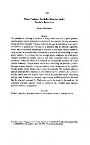
low), and a cost function which provides a realistic model net regression. The particle filter and subsequent Viterbi of impact and spread. We chose the model of Kyle and estimation ran in a few seconds on a notebook computer. Obizhaeva (2011) for this example because it is theoretitrading paths cally justified by basic microstructure invariance assumptions, and it was fit to a large data set of portfolio tran40000 sitions, hence it also has empirical support. variable For simplicity we assume that the asset being traded is 0 Viterbi the “benchmark asset” which Kyle and Obizhaeva (2011) Kalman use to center their model. This asset has price P = 40, −40000 daily volatility of σ = 0.02, and average daily volume 6 V = 10 shares. When using the reference asset, the 0 5 10 15 20 Kyle-Obizhaeva cost function simplifies to days

ct (δt ) = κ1 |δt | +

κ2 δt2 /(0.01P V

)

(21)

Figure 1: The solid line (“Kalman”) is the solution to a where we take κ1 = 2.89 × 10 and κ2 = 7.91 × 10 . quadratic-cost problem which has the highest true-utility With these parameter settings, the cost to trade one per- among all solutions to all quadratic-cost problems with cent of the average daily volume is 10.8 basis points of the same yt , γΣt . The dashed line (“Viterbi”) is the path the trade size. We assume an initial holding of x0 = 0 which optimizes true-utility over all possible paths. and take γ = 10−5 as our risk-aversion parameter. Our stylized alpha term structure is a simple sum of two Conclusions exponential-decay curves: model 1 is initially 25bps, with half-life 4 periods, while model 2 is initially −40bps with The framework presented here renders multiperiod opa shorter half-life of 2 periods. Adding these two models timization and multiperiod tracking problems computaproduces a term structure that is negative, then positive, tionally accessible, even with realistic costs such as bidthen decays to almost zero within about 20 periods. ask spread pay and nonlinear market impact. One of It is tempting to wonder whether a purely-quadratic the more striking conclusions is that a sequence of singleapproximation to cost (ie. κ1 = 0 and some other value asset trading path optimizations provably converges to of κ2 ) might suffice, since such a problem could be eas- the globally optimal multi-asset solution. ily solved by the Kalman smoother. However, such apIn our view, the main limitations of the model are proximations can be misleading. Consider the class of as follows. We treat the trading cost as non-stochastic, problems with the same yt , γ, and Σt as in the numerical whereas in real quantitative trading scenarios, a meanexample above, but with purely-quadratic costs; call this ingful part of the volatility (and higher moments) may the “quadratic class.” We propose that no solution in the arise from randomness in realized trading costs (or “slipquadratic class is particularly close to the solution which page”). Liquidity events such as August 2007, and the globally optimizes true utility (ie. utility computed with subsequent return of liquidity, provide empirical evidence the non-quadratic cost function), and that the closest is that realized slippage has meaningful left and right tails. the solid line shown in Fig. 1. The model as presented here does not take into account The best possible Kalman path (solid line) places a investors’ aversion to such higher moments. In a related limitation, the model is formulated as if larger number of trades than the Viterbi path, but the individual trades are smaller. This is because the purely- we expect to completely fill each order. Hence it does not quadratic approximation is over-estimating the cost of attempt to find the optimal solution for a passive execularge trades and under-estimating the true cost of small tion strategy in which order fill percentages are stochastrades relative to (21), which happens to be closer to lin- tic. This is of great interest, however, as passive strateear in the region of interest. The absolute-value term in gies typically pay lower costs on the orders that are filled. (21) allows sparse solutions, as is familiar from elastic- These represent exciting directions for future research. −4

February 11, 2015

−4

6

References Almgren, Robert and Neil Chriss (1999). Value under liquidation. In: Risk 12.12, pp. 61–63. Almgren, Robert et al. (2005). Direct estimation of equity market impact. In: Risk 57. Bellman, R. (1957). Dynamic Programming. Princeton University Press, Princeton, NJ. Black, Fischer and Robert Litterman (1992). Global portfolio optimization. In: Financial Analysts Journal, pp. 28–43.

February 11, 2015

Doucet, Arnaud and Adam M Johansen (2009). A tutorial on particle filtering and smoothing: Fifteen years later. In: Handbook of Nonlinear Filtering 12, pp. 656– 704. Gârleanu, Nicolae and Lasse Heje Pedersen (2013). Dynamic trading with predictable returns and transaction costs. In: The Journal of Finance 68.6, pp. 2309–2340. Godsill, Simon, Arnaud Doucet, and Mike West (2001). Maximum a posteriori

7

sequence estimation using Monte Carlo particle filters. In: Annals of the Institute of Statistical Mathematics 53.1, pp. 82–96. Kyle, Albert Pete and Anna Obizhaeva (2011). Market Microstructure Invariants: Theory and Implications of Calibration. In: Available at SSRN 1978932. Tseng, Paul (2001). Convergence of a block coordinate descent method for nondifferentiable minimization. In: Journal of optimization the-

ory and applications 109.3, pp. 475–494. Viterbi, Andrew (1967). Error bounds for convolutional codes and an asymptotically optimum decoding algorithm. In: Information Theory, IEEE Transactions on 13.2, pp. 260–269. Zakamouline, Valeri and Steen Koekebakker (2009). A Generalisation of the MeanVariance Analysis. In: European Financial Management 15.5, pp. 934–970.