Multiple Capacity Vehicle Routing on Paths

Multiple Capacity Vehicle Routing on Paths D. J. Guan and Xuding Zhu Department of Applied Mathematics National Sun Yat Sen University Kaoshiung, Taiwan 80424 R. O. C. {guan,zhu}@math.nsysu.edu.tw

March 21, 1997 Abstract Consider the problem of transporting a set of objects between the vertices of a simple graph by a vehicle that traverses the edges of the graph. The problem of finding a shortest tour for the vehicle to transport all objects from their initial vertices to their destination vertices is called the vehicle routing problem. The problem is multiple capacity if the vehicle can handle more than one objects at a time. The problem is preemptive if objects can be unloaded at the intermediate vertices. In this paper, we present an O(kn + n2 ) time algorithms for multiple capacity preemptive vehicle routing problem on paths, where k is the number of objects to be moved and n is the number of vertices in the path. Keywords. Vehicle routing, motion planning, graph algorithms. AMS Subject Classification: 05C85, 05C90, 68Q25.

i

1

Introduction

Consider an edge weighted graph with objects located at some vertices. Associated with each object is a destination vertex, to which that object is to be moved by a vehicle that traverses the edges of the graph. A fundamental problem in motion planning is to determine a tour of minimum cost for the vehicle to transport all objects from their initial positions to their destinations. The determination of a minimum cost tour for the problem is called the vehicle routing problem, and we are interested in the computational complexity of the vehicle routing problems. One factor that affects the complexity of the vehicle routing problem is whether or not we allow drops in the process of transportation. A drop is an unloading of an object at a vertex that is not its destination. If an object is dropped, its movement is not immediately completed, and the object will be picked up and transported farther at some later time in the transportation. Based on whether or not we allow drops in the transportation, we have two versions of the vehicle routing problems. We shall use nonpreemptive to denote the version in which no objects can be dropped at intermediate vertices, and preemptive to denote the version in which objects can be dropped at intermediate vertices. Another factor that makes a difference on the complexity of the vehicle routing problem is whether the capacity of the vehicle is 1, or greater than 1. Suppose the vehicle can transport c objects at a time. We refer the problem as unit capacity vehicle routing problem if c = 1; and refer it as multiple capacity vehicle routing problem if c ≥ 2. Combined with the preemptive version and nonpreemptive version, we have four kinds of vehicle routing problems: unit capacity preemptive vehicle routing problem, unit capacity nonpreemptive vehicle routing problem, multiple capacity preemptive

1

vehicle routing problem and multiple capacity nonpreemptive vehicle routing problem. For general graphs, all the four problems are NP-hard [2]. However, for practical applications such as elevators and those that arise in robotics, it suffices to consider more restricted classes of graphs. Indeed, for all the recent research in this area, focus has been on solving the vehicle routing problems on paths, cycles and trees [1, 3, 4, 5, 6, 7]. The unit capacity (preemptive and nonpreemptive) vehicle routing problems on paths and cycles are shown to be polynomial time decidable by Atallah and Kosaraju [1] and Frederickson [3]. For unit capacity vehicle routing problem on trees, Frederickson and Guan [4] proved that the preemptive version is polynomial time decidable, while the nonpreemptive version is NP-complete. For multiple capacity nonpreemptive vehicle routing problems, Gaun [6] proved that the problem is NP-complete even if the underlying graph is a path. This of course implies that the problem is NP-complete on cycles and trees. Summing up the results above, the only cases that remain open are the multiple capacity preemptive vehicle routing problems on paths and cycles. (Note that multiple capacity nonpreemptive routing problem on trees is NP-complete, as an instance of unit capacity nonpreemptive routing problem on trees can be easily reduced to a multiple capacity preemptive routing problem on trees.) The multiple capacity preemptive routing problem on paths were investigated by Karp [7] and Guan [6]. Karp constructed a polynomial time algorithm for this problem under two constraints: (1) the starting vertex is an endpoint of the path; (2) the number of objects located at each vertex before and after the transportation should be the same. In [6], Guan analyzed the time complexity of Karp’s algorithm, and showed that the algorithm takes O(kn log log n) time, where k is the number of 2

objects and n is the number of vertices. Then Guan constructed an algorithms with time complexity O(k + n), and which does not require that the number of objects located at each vertex before and after the transportation be the same. However, it is crucial for both Karp’s and Guan’s algorithms that the starting vertex is an end vertex of the path. In this paper, we give a polynomial time algorithm for the multiple capacity preemptive routing problem on paths, without imposing any constraints. The time complexity of our algorithm is O(kn + n2 ). Then we go on to show that our algorithm can actually be applied to the multiple capacity preemptive routing problem on cycles, under the constraint that for each object the direction of transportation is given. (Note that to transport an object from vertex i to vertex j on a cycle, we can go either the clockwise direction or the counterclockwise direction.) We remark that in practice, an object is usually transported along the shorter arc connecting the two vertices. Thus the constraint is not very unnatural. However, there are cases that we can reduce the cost by allowing some objects go along the longer arc connecting their initial positions and destinations.

2

Preliminary

An instance of a vehicle routing problem consists of an edge weighted graph G, a set O of objects together with their initial positions and destinations, a designated vertex s of G which is the starting position as well as the ending vertex of the vehicle, and a constant c which is the capacity of the vehicle. The weight of an edge represents the distance or the cost of transporting the objects between the two vertices of the edge and which is assumed to be non-negative. We shall assume throughout the paper that the number of vertices of the graph G is n and that the number of objects is k. We 3

shall concentrate on the case that the graph G is a path whose vertices are labeled 1, 2, . . . , n, where (i, i + 1), i = 1, 2, . . . , n − 1, are the edges of G. The k objects will also be labeled by 1, 2, . . . , k. The initial vertex and destination vertex of object j are uj and vj , respectively. We represent an object j by a directed edge from uj to vj with label j. Thus an instance of a vehicle routing problem can be represented by a mixed graph which has undirected edges as well as directed edges. Each undirected edge has a non-negative weight, and each directed edge has a label from the integer set {1, 2, . . . , k}. A move from a vertex x to a vertex y of the vehicle carrying a set of objects Z is designated by (x, y; Z). Each move (x, y; Z) with Z 6= ∅ is called a carrying move, otherwise, it is called a non-carrying move. Let c be the capacity of the vehicle. A carrying move with |Z| = c is called a full-carrying move. An object j is transported from x to y by a move (x, y; Z) if j is at vertex x before the move, and j ∈ Z. After the move, the object j will be at vertex y. A transportation, Q from v0 to vr , is a sequence of moves Q = (v0 , v1 ; Z1 ), (v1 , v2 ; Z2 ), . . . , (vr−1 , vr ; Zr ).

Let Q be a transportation. Let Q(j) be a subsequence of moves obtained from Q by deleting those moves that does not involve the object j. An object is transported from x to y by a transportation Q, if Q(j) is a transportation from x to y. If objects cannot be dropped at the intermediate vertices, then Q(j) must be a consecutive subsequence of moves of Q. A transportation is em valid, if v0 = vr = s, and each object is transported 4

from its initial position to its destination by Q. Unless stated otherwise, we consider only valid transportations, and we should use transportation, instead of valid transportation. The cost of the transportation, c(Q), is the distance the vehicle traversed. That is, c(Q) =

r X

d(vi−1 , vi ),

i=1

where d(vi−1 , vi ) is the sum of the weights of the edges from vi−1 to vi in the underlying graph. A transportation Q is an optimal transportation if c(Q) is minimum among all valid transportations. The vehicle routing problem is to find an optimal transportation. Let L be the underlying graph. Denote L[l, r] the subgraph of L induced by the vertices l, l + 1, . . . , r. Let L[u, v] and L[x, y] be two disjoint subgraphs of L. Define f ([u, v], [x, y]) to be the number of objects with initial position in L[u, v] and destinations in L[x, y]. Since the underlying graph is a path and the vehicle must return to s, each edge must be traversed by the vehicle at least twice, once in each direction. Furthermore, for each edge (u, v), the number of times the vehicle traverses the edge from u to v must be equal to the number of times the vehicle traverses the edge from v to u. We, therefore, define a balanced problem as follows. For each edge e = (v, v + 1), let λe = max{df ([1, v], [v + 1, n])/ce, df ([v + 1, n], [1, v])/ce, 1}. That is, λe is the minimum number of times that the vehicle must traverse the edge e in either direction. A problem with f ([1, v], [v + 1, n]) = f ([v + 1, n], [1, v]) = cλe , for each edge e = (v, v + 1), v = 1, 2, . . . , n − 1, is called a balanced problem. 5

1m

2m 1

3m

4m

5m

6m

-

2

3

-

4

-

5

-

6

-

7

-

8

-



9



10



11



12

7m

-

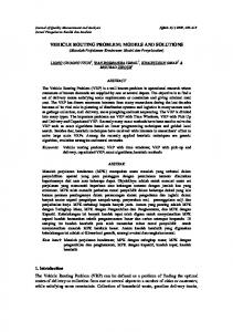
Figure 1: An example of the vehicle routing problem. Given an arbitrary instance of the vehicle routing problem, one can add objects to make it into a balanced problem without increasing the cost of an optimal transportation. A trivial method is to add cλe −f ([1, v], [v+1, n]) objects to be transported from v to v + 1, and add cλe − f ([v + 1, n], [1, v]) objects to be transported from v + 1 to v, for each edge e = (v, v + 1). It is clear that the total number of objects added to the problem is at most kn/2 and it can be done in O(kn) time. For the remaining part of this paper, we shall only consider balanced problems. Figure 1 is an example of vehicle routing problem, where the weight of each undirected edge is 1, the capacity of the vehicle is 2. For clarity, directed edges are drawn with vertical offsets. If the starting vertex is 1, then it is easy to verify that the following sequence of moves is a transportation of the given problem: (1, 2; {1, 3})(2, 4; {5, 7})(4, 6; {6, 8}) (6, 2; {9, 10})(2, 3; {1, 3})(3, 5; {2, 3})(5, 7; {2, 4})(7, 1; {11, 12}). Note that this transportation consists of only full-carrying moves and each object is transported in such

6

a way that it traverses the edges between its initial vertex and its destination vertex exactly once, and traverses no other edges. Therefore, this is an optimal transportation. Indeed, it was proved in [6] that for any balanced multiple capacity preemptive vehicle routing problem on a path there is a transportation that consists of only full-carrying moves. For the application in this paper, we shall briefly describe the algorithm given in [6], which are divided into two steps: 1. First we use a greedy algorithm, which starts at 1, and which arbitrarily picks c objects whose destinations are on the same side of the current vertex, and move them toward their destinations. The vehicle repeatedly moves objects in this direction. It changes the direction of movement only if, at the current vertex, there is not enough objects to be moved in the current direction. It was proved in [6] that if there is not enough objects to be moved to either direction, then the current vertex must be the starting vertex. In other words, the route of the vehicle is a closed walk of the underlying graph. Since the problem is balanced, when the above procedure stops, none of the remaining objects will be transported through the first edge. In other words, the first edge and hence the first vertex are irrelevant to the remaining problem. Let x be the first vertex which is relevant to the remaining problem. Then we start from vertex x, and apply the above greedy algorithm again, to obtain another sequence of moves, which form another closed walk of the underlying graph. Repeat this process to obtain a sequence of closed walks that together move every object to its destination. 2. As the second step, we cut and past these closed walks to form a single closed walk. This is very similar to the algorithm that finds an Euler tour of an 7

Eulerian graph. This single closed walk corresponds to a transportation which consists of only full-carrying moves. We remark that the algorithm above does not work if the starting vertex is not an end vertex of the path. Indeed, in Example 1, if the starting vertex s = 4, then there is no transportation in which all moves are full-carrying moves. We shall show how to compute an optimal transportation for the case that the starting vertex is not at the end-point of the path in the following section.

3

Preemptive Routing in Paths

In this section, we present an O(kn+n2 ) time algorithm to solve the multiple capacity preemptive vehicle routing problem on paths. We shall first establish a necessary and sufficient condition for a balanced problem to have a transportation that consists of only full-carrying moves. Theorem 1 Let P be a balanced instance of a multiple capacity vehicle routing problem on a path, in which the starting position of the vehicle is s. There is a transportation that consists of only full-carrying moves if and only if there exists a sequence of full-carrying moves from s to one of the end-points of the path. Proof

If P has a transportation Q that consists of only full-carrying moves that

starts from s, then of course there exists a sequence of full carrying moves from s to one of the end-points of the path. Assume that there exists a sequence of full carrying moves, say Q1 , from s to one of the end vertex, say 1. Let P 0 be the problem resulting from P by performing the sequences of moves in Q1 , and let P 00 be the problem obtained from P 0 by adding

8

¯ the set of c objects with initial vertex s and destination vertex 1. We denote by X added objects. The problem P 00 is “almost” balanced, except that there might be somes edges e for which λe = 0. For simplicity, we may assume that the problem P 00 is indeed balanced. In case there are edges e for which λe = 0, we only need to consider each sub-problem separately, and at the final stage, to combine the sub-transportation together. This is a quite routine process, and the same technique is also used in Guan’s algorithm described in the previous section. Now let P¯ be the problem obtained from P 00 by switching the initial position ¯ now have initial position 1 and the destination of each object. Thus the objects of X and destination s. Apply the algorithm described in the previous section to P¯ in such ¯ from 1 to s. Also when applying the second a way that the very first step moves X step of the algorithm to combine sub-transportations into a single transportation, we ¯ This is possible because objects in X ¯ are shall avoid splitting the move (1, s; X). added to make the problem balanced, and hence the vertices between s and 1 must ¯ be traversed by the vehicle transporting objects not in X. ¯ 0 . Let Q ¯ be Let the optimal transportation obtained by the algorithm be Q ¯ 0 , which is defined as the inverse of the sequence of the moves in Q the inverse of Q ¯ is a valid and each move (x, y; Z) is transformed into (y, x; Z). It is clear that Q transportation of P 00 that consists of only full-carrying moves. An optimal transportation for the original problem, starting and ending at ¯ by replacing the last move, which is the move for vertex s, can be obtained from Q ¯ with the sequence Q1 of full-carrying moves. the objects in X, Now we present an algorithm that determines whether or not there exists a sequence of full-carrying moves from s to 1 or n. 9

We say a vertex x of the path is reachable (from s) if there is a sequence of full-carrying moves from s to x. Suppose x is a reachable vertex. We define the predecessor p(x) of x as follows: If x ≥ s, then p(x) is the largest vertex such that p(x) ≤ s and any sequence of full-carrying moves from s to x pass through p(x). If x < s, then we define p(x) to be the smallest vertex such that p(x) ≥ s and any sequence of full-carrying moves from s to x pass through p(x). Intuitively, if there is a sequence of full-carrying moves from s directly to x, then p(x) = s. Otherwise, to have a sequence of full-carrying moves from s x, the vehicle may need to visit the vertices beyond s in order to pick up the necessary objects. The predecessor p(x) is the vertex closest to s such that the vehicle makes its last turn before reaching x. Note that the predecessor function p(x) is monotone, in the sense that if x ≤ y ≤ s then p(x) ≥ p(y); and if x ≥ y ≥ s then p(x) ≤ p(y). This monotone property reduces the computational complexity in finding an optimal transportation. Suppose x is a reachable vertex. We define a function cx : E → Z + , which is the smallest number of times the vehicle traverses the edge e, in the direction away from s, before it can reach the vertex x. The number of times the vehicle traverses the edge e in the direction towards s will not be counted in cx (e). The values of cx (e) are computed as follows. Initially, let cs (e) = 0 for every edge e ∈ E. Suppose p(x) is known and that cp(x) (e) is determined for each edge e. The value of cx (e) can then be computed as follows. For x 6= s, cx (e) = cp(x) (e) + 1 if the edge e is between the two vertices s and x, otherwise, cx (e) = cp(x) (e). It can be proved by induction on

X

cx (e) that for each reachable vertex x,

e∈E

there is a sequence of full-carrying moves from s to x that traverses the edge e in the 10

direction away from s exactly cx (e) times, and any other full-carrying moves from s to x traverses the edge e in the direction away from s at least cx (e) times. Therefore, the vehicle must traverse each edge e cx (e) times, in the direction away from s, before reaching x. The algorithm that determines the reachable vertex, the predecessor p(x), and the value of cx (e) for each reachable vertex x is described as follows. The algorithm keeps track of a set R, which is the set of currently known reachable vertices. By the definition of reachable vertex, the induced subgraph P [R] must be a connected subpath of P , which includes the start vertex s. We shall use the notation R = [l, r] to denote the set of researchable vertices l, l + 1, . . . , r. Initially, R = [s, s], p(s) = s, and cs (e) = 0 for every e ∈ E. Suppose that at the i-th iteration, R = [l, r]. Then, in the (i + 1)-th iteration, the algorithm checks whether or not the vertex l − 1 and the vertex r + 1 are reachable or not. The testing of whether the vertex l − 1 is a reachable vertex or not is described as follows. For each vertex x = p(l), p(l) + 1, . . . , r, the algorithm decides whether or not there is a sequence of full-carrying moves from s to x and then directly from x to l − 1 (i.e., without making another turn). We should prove that there is such a sequence of full carrying moves if and only if the following conditions are satisfied. 1. For each edge e = (a, b) ∈ E between s and l − 1, we have c · (cx (e) + 1) ≤ f ([b, x], [1, a]). 2. For each edge e = (a, b) ∈ E between s and x, we have c · cx (e) ≤ f ([b, x], [1, a]). If the inequalities above hold for all the edges e between x and l − 1, then the algorithm adds l − 1 to R, (that is, change R from [l, r] to [l − 1, r].) set p(l − 1) = x, 11

and set cl−1 (e) = cx (e) + 1 for those edges e between s and l − 1, and set cl−1 = cx (e) for other edges e. If the inequalities above do not hold for some edge e between x and l − 1, then the vertex l − 1 cannot be reached before the vehicle going further to the right of x. Thus the algorithm increases the value of x provided that x < r, and then repeats the procedure above. If x = r, the vertex l − 1 cannot be reached at the moment, and the algorithm starts checking whether r + 1 is a reachable vertex or not. The method for checking whether or not r + 1 is a reachable vertex is similar to the case for the vertex l − 1. The algorithm repeatedly checking if the end-points of R can be extended or not, and the algorithm stops when neither l − 1 nor r + 1 is reachable. We shall show that the algorithm above indeed finds all reachable vertices. Theorem 2 Let P be a balanced problem. At the end of the the algorithm, the interval R contains all reachable vertices. In other words, for each x ∈ R, there is a sequence of full-carrying moves from s to x; and for any x 6∈ R, there does not exist such a sequence of full-carrying moves. Proof

For simplicity, we may assume that x ≤ s. We shall prove by induction the

following stronger statement: For each x ∈ R, x ≤ s, there is a sequence of full-carrying moves from s to x, in which the vehicle traverses each edge e exactly cx (e) times along the direction away from s, and that p(x) is the largest vertex that the vehicle passes through before reaching x. Moreover, for any other sequence of full-carrying moves from s to x, the vehicle traverses each edge e at least

12

cx (e) times along the direction away from s, and that the vehicle must pass through p(x) before reaching x. For x > s, a corresponding result holds. Although in our argument we only consider vertices x ≤ s, our induction hypothesis is for all vertices added to R before the vertex x is added. At the initial step, R = [s, s], and the statement above is obviously true. Suppose x is added to R at step i. Then p(x) ≥ s is added to R at some previous step, and hence the statement above is true for any vertex y between s and p(x) by the induction hypothesis. Thus there is sequence of full-carrying moves from s to p(x) that traverses each edge e exactly cp(x) (e) times along the direction away from s. Now we shall extend such a sequence by adding some full-carrying moves from p(x) to x (without making turns). Of course the only concern is that whether or not there are enough objects to be picked up and moved along the way. There are such objects for the following two reasons: 1. The previous sequence of moves traverses each edge e = (a, b) ∈ E between s and p(x) exactly cp(x) (e) − 1 times in the direction from p(x) to x (note that for these edges, this is the direction towards s, and that the vehicle starts at s), and traverses each edge e = (a, b) ∈ E between s and x exactly cp(x) (e) times in direction from p(x) to x. 2. For each edge e = (a, b) ∈ E between s and p(x), we have c · cx (e) ≤ f ([b, x], [1, a]) holds for each edge e = (a, b) ∈ E between s and p(x), and for each edge e = (a, b) ∈ E between s and x, we have c · (cx (e) + 1) ≤ f ([b, x], [1, a]). 13

Next we show that each sequence of full-carrying moves from s to x must pass through p(x). Assume to the contrary that there is a sequence of full-carrying moves to x and that the maximum vertex that the vehicle passes through is y < p(x). Then an initial segment of this sequence forms a sub-sequence of full-carrying moves from s to y. By the induction hypothesis, for each edge e = (a, b) ∈ E between s and x, this sub-sequence of moves traverses e at least cy (e) times along the off s direction; and for each edge e = (a, b) ∈ E between y and s, this sub-sequence of moves traverses e at least cy (e) − 1 times along the towards s direction. On the other hand, it follows from the algorithm that, since p(x) > y, there is either an edge e = (a, b) ∈ E between s and x such that c · (cx (e) + 1) > f ([b, x], [1, a]), or there exists an edge e = (a, b) ∈ E between s and y such that c · cx (e) > f ([b, x], [1, a]). In either case, there are not enough objects to be picked up on the way for the vehicle to pass through the edge e. Therefore, every sequence of full-carrying moves from s to x pass through p(x). The argument above can be easily modified to show that every sequence of full-carrying moves from s to x traverses each edge e at least cx (e) times along the off s direction. We shall omit the details. Also the argument above can be modified to show that for any vertex x 6∈ R, there exists no sequence of full-carrying moves from s to x, and we shall omit the details. As shown by Example 1, for some balanced problems, it is possible that there does not exist a transportation which consists of only full-carrying moves. By Theo14

rem 1, for such a problem, there does not exist a sequence of full-carrying moves from s to an end-point of the path. In other words, the vertices 1 and n are not reachable. For such problems, the optimal transportation must contain moves (x, y; Z) with |Z| < c. It is straightforward to verify that, for balanced problems, we may restrict to full-carrying moves and non-carrying moves. To determine a minimum cost transportation for a problem, it suffices to determine the minimum distance traveled by the vehicle with non-carrying moves. As each edge must be traversed by the vehicle the same number of times in both directions and that the original problem is balanced, we conclude that for each edge e, the number of times the vehicle traverses e in the two directions with a non-carrying move is equal. Thus we may just count the number of times the vehicle traverses the edge e in the off s direction with a non-carrying move. We define the cost of a non-carrying move to be the distance of that move. Suppose there is a vertex x of the path which is not reachable. We define c(x) to be the minimum cost reaching x, i.e., the minimum total distance that the vehicle needs to travel with non-carrying moves before reaching x. We shall present an algorithm that determines recursively the values of all c(x). Before we present the algorithm, we consider again the example shown in Figure 1. Assume that the capacity of the vehicle c = 2. If the start vertex s = 6, then all the vertices are reachable vertices. However, if the start vertex s = 4, then the reachable set R = [2, 6]. Readers are advised to try to find the minimum cost of adding objects to make each of the other vertices reachable. In the algorithm, we keep track of the following parameters: S : the set of vertices whose optimal cost have already been computed.

15

v : the last vertex added to S. c(x) : the current known minimum cost of reaching x; cx (e) : the current known minimum number of times the vehicle traverses the edge e, in the direction away from s, in order to reach the vertex x with the cost c(x); x (e) : the currently known minimum number of times the vehicle crosses the edge e in the off s direction with a non-carrying move, in order to reach x. Our algorithm is similar to the Dijkstra’s algorithm for finding the shortest path between two vertices in a weighted graph. The above parameters will be updated at each iteration. Note that S must be a connected subgraph of the path, hence S = [l, r] is always an interval. Initially, we set S = [s, s], v = s, c(s) = 0, cs (e) = 0 and s (e) = 0 for every e ∈ E. For each x 6= s, we let c(x) = ∞, cx (e) = ∞ and x (e) = ∞ for every edge e. At each iteration, the parameters are updated by the following rules: If v ≤ s, then for each vertex x 6∈ S and x > s, we calculate the cost c0 (x) of moving the vehicle from s to x in such a way that the vehicle reaches v first (with cost c(v)) and then goes directly from v to x (with some additional cost that can be calculated easily). Then we compare the new cost c0 (x) with the current value c(x), and replace it with c0 (x) if c0 (x) < c(x). If v ≥ s, then we use the value of c(v) to update the cost of c(x) for all x < s, in the same way. After we finished updating the cost function, then we add the vertex x with the minimum cost c(x) among the vertices V − S into S, and then repeat the above process again.

16

This is exactly what was done in the the Dijkstra’s algorithm for finding the shortest path between two vertices in a weighted graph. However, we need some tools to calculate the cost c0 (x). In order to calculate the additional cost of moving the vehicle from v to x, we need to know how many times the vehicle traverses each edge e along the direction from v to x. Then we determine if there are enough objects to be transported by the the vehicle to cross the edge. In case there is not enough objects to be transported by the vehicle to cross the edge e = (a, b), then the vehicle needs to cross the edge e with a non-carrying move, and that will contribute to the cost of reaching x. As noted before, we may just count the number of times the vehicle traverses the edge e in the off s direction with a non-carrying move. We shall not consider the cost of moving the vehicle towards s. Let gx,v (e) be the minimum number of times the vehicles traverses the edge e in the direction from v to x, under the condition that the vehicle first reaches v and then directly goes to x. Then since cv (e) is the minimum number of times the vehicle traverses the edge e in the off s direction in the process of going from s to v, we conclude that: 1. for edges e between v and s, gv,x (e) = cv (e), and 2. for edges e between s and x, gv,x (e) = cv (e) + 1. Assume that v ≤ s < x. Let W (v, x) be the set of edges e = (a, b) between s and x such that f ([v, a], [b, n]) < c · (gv,x (e) − v (e)). Then it is clear that W (v, x) is the set of edges that the vehicle needs to traverse with a non-carrying move, along the way from v to x. (Note that f ([v, a], [b, n]) is the total number of objects that can be transported from a to b at present time; gv,x (e) is the total number of times 17

the vehicle traversed from a to b up to now, including the trip from v to x; and v (e)) is the total number of times the vehicle has already traversed from a to b with non-carrying moves.) X

Thus, we set c0 (x) = c(v) +

w(e). Then we compare c0 (x) with c(x). In

e∈W (v,x)

case that c0 (x) < c(x), we set c(x) = c0 (x); and set x (e) = v (e) for e 6∈ W (v, x) and x (e) = v (e) + 1 for e ∈ W (v, x); and set cx (e) = cv (e) if e is between v and s, and cx (e) = cv (e) + 1 if e is between x and s. Find a vertex x in V − S such that c(x) = min{c(y) : y ∈ V − S}, and then let S = S ∪ {x}. Then we set v = x, and repeat the procedure above. The algorithm terminates when one of the end vertices of the path is added to S. Without loss of generality, we assume that 1 is added to S. Then 2c(1) is the minimum distance that must be traveled by the vehicle with non-carrying moves in any transportation for the problem. Theorem 3 The algorithm described above indeed determines the minimum distance that must be traveled by the vehicle with non-carrying moves in any transportation for the problem. Proof

First we note that there is a transportation for the problem in which the

total distance traveled by the vehicle with non-carrying moves is 2c(1). Indeed, in the process of reaching 1 by taking some non-carrying moves, we may replace each non-carrying move that cross an edge e = (a, b) in the off s direction by the addition of c objects from a to b, and c objects from b to a. Then after these objects are added, the resulting problem is still balanced and that in this problem the vertex 1 becomes a reachable vertex. Then by Theorem 1, there is a transportation for this new problem that consists of only full-carrying moves. By omitting those added objects, we obtain 18

a transportation of the original problem in which the total distance traveled by the vehicle with non-carrying moves is 2c(1). Next we shall show that in any other transportation, the total distance traveled by the vehicle with non-carrying moves is at least 2c(1). Since in any transportation, the vehicle must reach vertex 1, it suffices to show for the vehicle to reach the vertex 1, it has to travel a distance of at least c(1) in the off s direction, with non-carrying moves. We shall show by induction that for each vertex x of S, the vehicle needs to travel a distance of at least c(x) in the off s direction, before reaching x. Suppose S ∗ is the set of vertices of S which are added to S before x, and suppose to the contrary of the theorem that there is a sequence of moves, say Q1 , for the vehicle to reach x with less non-carrying move distance. By the induction hypothesis, and by the procedure of updating the value of c(x), it is straightforward to see that in the sequence of moves Q1 , the vehicle must reach some vertex y 6∈ S ∗ before reaching x. Let y0 be the first vertex not in S ∗ which is reached by the vehicle in this sequence of moves. Then it follows from the induction hypothesis and the procedure for defining c(y) at that step, we conclude that the total distance traveled by the vehicle with non-carrying moves along the off s direction is at least c(y) ≥ c(x), which is a contradiction. Here c(y) is the value at the step we add x into S. (Recall that in the algorithm the value c(y) is updated at each step.)

Theorem 4 The algorithm described above terminates in O(kn + n2 ) time, where k is the number of objects to be transported and n is the number of vertices in the path. Proof

After each iteration, one vertex is added to S. Hence there are at most n

iterations. The crucial step to make the algorithm efficient is to compute the values of f ([v, x], [x + 1, n]) and f ([v, x + 1], [1, x]) efficiently. We shall show how to compute 19

all the values of f ([v, x], [x + 1, n]), for v = s, s + 1, . . . , n, x = v, v + 1, . . . , n − 1, in O(kn + n2 ) time. The computation for f ([v, x + 1], [1, x]) for v = s, s − 1, . . . , 1, x = v − 1, v − 2, . . . , 1, is done in a similar way. For each vertex v, let α(v) be the set of objects with initial position v, and with destinations to the right of v. For v, x ∈ V , v < x, let βv (x) be the set of objects with initial positions between v and x − 1 and with destination x, let δ(v, x) be the set of objects with initial position v and with destination x. By definition, βv (x) = βv+1 (x) ∪ δ(v, x). For any given v, v ≤ s, the value of f ([v, v], [v + 1, n]) = |α(v)|, and for x = v + 1, v + 2, . . . , n − 1, f ([v, x], [x + 1, n]) = f ([v, x − 1], [x, n]) + |α(x)| − |βv (x)|. After balancing objects are added, there are at most O(kn) objects. It is straightforward to compute all the values of δ(v, x), for all v, x ∈ V , in O(kn + n2 ) time. After these values are computed, for any given v, the values of f ([v, x], [x + 1, n]), x = v, v + 1, . . . , n − 1, can each be computed in constant time. Therefore, our algorithm can be implemented in O(kn + n2 ) time. An analysis of the algorithm shows that we have the term kn in the time complexity, simply for the reason that we may add O(kn) objects to make it a balance problem. We remark that with a complex algorithm, we can produce a balanced problem in which the number of added objects is at most O(k + n). If we use that algorithm to produce the balance version (which we did not use for the reason of simplicity), the time complexity of our algorithm can be reduced to O(k + n2 ).

20

4

Preemptive Routing on Cycles

We shall show in this section that the algorithm in the previous section can be applied to the multiple capacity preemptive vehicle routing problems on cycles, provided that the arc along which each object is to be transported is determined. In practice, we usually transport an object along the shorter one of the two arcs connecting its initial position and its destination. We assume that the cycle has vertices 1, 2, . . . , n, embedded in the plane in this order along the clockwise direction. Unlike the path, for a vehicle to starts and ends at a vertex s of a cycle, it is not necessary that the vehicle traverses each edge the same number of times in both directions. This is because the vehicle can go around the cycle in one direction many times and return to the staring vertex. We shall employ techniques of [1] for overcoming this difficulty. First we modify the definition of a balanced problem. Let e be an edge of the cycle C, λ(e) be the number of objects that must traverse the edge e in clockwise direction, and λ0 (e) be the number of objects that must traverse the edge e in counterclockwise direction. A problem is balanced if, and only if, for each edge e of C, λ(e) ≡ λ0 (e) ≡ 0 mod c and φ(e) = λ(e) − λ0 (e) = cψ, where c is the capacity of the vehicle and ψ is a constant. The algorithm for finding an optimal tour is summarized as follows. First, find the balanced version of the problem for some fixed value of ψ. Using the algorithm for the paths, find a sequence of moves with minimum total distance of non-carrying 21

moves such that the vehicle visit all the vertices of the cycle. Similarly we define c(x) to be the minimum total distance of non-carrying moves to reach x. Let v be the vertex with largest cost c(v) among all vertices in C. Then similar to Theorem 3, it can be proved that 2c(v) is the minimum total distance traveled by a vehicle with non-carrying moves in a transportation for the problem, under the condition that the vehicle goes around the cycle in the clockwise direction ψ times. ( ) ( ) λ0 (e) λ(e) For each number ψ between − max + 1 and max + 1 , we ape∈E e∈E c c ply the above algorithm. At the very end we choose the value of ψ for which the corresponding cost is minimum. That will be the minimum cost of a transportation for the problem. We remark that this algorithm works only if each object is moved in the predetermined direction. The general problem remains open. In addition to this problem, we list two more open problems: 1. Suppose the underlying graph G is obtained from a fixed number, say k, of paths by joining one of their end points together. In other words, G is like a star, with a constant number of branches. What is the complexity of multiple capacity preemptive vehicle routing problems on G? We note that if the number of branches is not a constant, then the problem was shown to be NP-complete [6]. 2. Suppose the capacity of the vehicle is unlimited, then what is the complexity of the vehicle routing problem on some special graphs such as trees or graphs of bounded tree-width? We note that this problem is easily seen to be polynomial on paths and cycles, and NP-complete for general graphs.

22

References [1] M. J. Atallah and S. R. Kosaraju. Efficient solutions to some transportation problems with application to minimizing robot arm travel. SIAM Journal on Computing, 17(5):849–869, 1988. [2] G. N. Frederickson, M. S. Hecht, and C. E. Kim. Approximation algorithms for some routing problems. SIAM Journal on Computing, 7(2):178–193, May 1978. [3] Greg N. Frederickson. A note on the complexity of a simple transportation problem. SIAM Journal on Computing, 22(1):57–61, 1993. [4] Greg N. Frederickson and D. J. Guan. Preemptive ensemble motion planning on a tree. SIAM Journal on Computing, 21(6):1130–1152, December 1992. [5] Greg N. Frederickson and D. J. Guan. Nonpreemptive ensemble motion planning on a tree. Journal of Algorithms, 15(1):29–60, July 1993. [6] D. J. Guan. Routing a vehicle of capacity greater than one. Technical report, Departmant of Applied Mathematics, National Sun Yet-Sen University, 1996. [7] R. M. Karp. Two combinatorial problems associated with external sorting. In R. Rustin, editor, Combinatorial Algorithms, Courant Computer Science Symposium 9, pages 17–29. Algorithmics Press, New York, January 1972.

23