Multiple Observer Siting and Path Planning on a. Compressed Terrain. Daniel M. Tracya, W. Randolph Franklinb, Barbara Cutlera, Marcus Andradeb,c, Franklin ...
Multiple Observer Siting and Path Planning on a Compressed Terrain Daniel M. Tracya , W. Randolph Franklinb , Barbara Cutlera , Marcus Andradeb,c , Franklin T. Luka , Metin Inanca , and Zhongyi Xiea a Department b Department
of Computer Science, Rensselaer Polytechnic Institute; of Electrical, Computer, & Systems Engineering, Rensselaer Polytechnic Institute c Universidade Federal de Vi¸ cosa, Vi¸cosa, Brazil ABSTRACT
We examine a smugglers and border guards scenario. We place observers on a terrain so as to optimize their visible coverage area. Then we compute a path that a smuggler would take so as to avoid detection, while also minimizing the path length. We also examine how our results are affected by using a lossy representation of the terrain instead. We propose three new application-specific error metrics for evaluating terrain compression. Our target terrain applications are the optimal placement of observers on a landscape and the navigation through the terrain by smugglers. Instead of using standard metrics such as average or maximum elevation error, we seek to optimize our compression on the specific real-world application of smugglers and border guards.
1. INTRODUCTION The usual way to evaluate a compression scheme is to calculate the per-pixel average and the maximum errors between the original and reconstructed geometry. This metric may not be appropriate for the common tasks performed on terrain data. It may be beneficial to consider more domain-specific applications. For example, visibility is can be useful for surveying, cell phone tower placement, military surveillance, etc. We consider the problem of multiple observer siting on a compressed terrain. An observer is placed at a point on the terrain and can see other points on the terrain only if no other part of the landscape obstructs a direct line of sight to the points, and the point is within the radius of visibility. Typically, the observer is placed at a specified height above the terrain, and lines of sight are drawn out to targets that are also a specified height above the terrain. In a highly mountainous terrain, points within narrow valleys typically have low visibility. The problem is to site a group of observers so as to maximize the amount of visible terrain; an application is the placement of watchtowers to observe a territory. In many real world scenarios, this problem must be solved using only the compressed terrain because the original terrain requires too much storage. For our problem, we want to evaluate the quality of the reconstructed geometry provided by the compression scheme. In this paper, we propose a new test protocol and new error metrics. Our new protocol is to compute a minimum-length path from the northwest corner of the terrain to the southeast corner, while avoiding detection, and our new error metrics are to examine path lengths and visibility errors.
2. TERRAIN COMPRESSION TECHNIQUES We consider a novel compression technique that we have developed, ODETLAP. We also examine JPEG, which was originally developed for image compression, but it has been repurposed and applied to other compression tasks. However, artifacts that are acceptable in the image domain could be probematic in terrain compression.
Figure 1. Example of a Triangulated Irregular Network
2.1 ODETLAP Franklin, Xie, and Inanc developed an alternate compression scheme, ODETLAP. It selects a set of control points and encodes them to generate the compressed format. A full terrain can then be lossily reconstructed from these control points through an interpolation scheme that can infer local maxima. The full details of this algorithm are described by Xie, et al.8 The main goal of ODETLAP (Overdetermined Laplacian) is to fill in gaps in the terrain, while making the terrain as smooth as possible. A overdetermined linear system is set up to solve the Laplacian equation, zxx + zyy = 0. For each grid point, the equation zi,j = (zi+1,j + zi−1,j + zi,j+1 + zi,j−1 )/4 is generated. Also, for each point whose elevation is prespecified as hi,j , the equation zi,j = hi,j is produced. This allows these points to drift slightly from their prespecified values. This can be useful for low-precision data sets that have erroneous terracing artifacts. ODETLAP can smooth away the terracing by allowing the points to take on intermediate values. Given k specified elevations on an n-by-n grid, ODETLAP generates n2 + k equations for n2 unknowns. One advantage of ODETLAP over competing interpolation schemes is that it is able to infer local maxima.
3. MULTIPLE OBSERVER SITING Next we consider the smugglers and border guards scenario in order to evaluate our compression scheme. In this game a team places a set of observers (guards) on the terrain, and the opponent, a smuggler, must plan a path to traverse the terrain from a starting point to a specified end point. The observers are assumed to be stationary. First we need a scheme for border guard placement. The goal is to place a set of observers on the terrain so as to maximize their joint viewshed, which is the area of the terrain that is visible by at least one observer. Due to the inherent complexity of computing the visibility between every pair of points on the terrain, it is impractical to compute the exact optimal solution to the multiple observer siting problem, especially when considering applications on small portable devices used by soldiers out in the field. Therefore, we employ the multiple observer siting algorithm developed by Franklin and Vogt,1 which uses a randomized algorithm to approximate the optimal siting of observers. There are several input parameters: R: The maximum radius of an observer’s visibility. In practice this may be limited by the transmission power of a cell tower, for example. H: The heights of the observers and targets. O: The maximum number of observers to site on the terrain. A: The minimum area to be covered by the observers. The algorithm is divided into four major steps: 1. Vix: The visibility of each point, which is known as the visibility index, is estimated using a Monte Carlo method. For each point, T points within the radius R are randomly sampled. For each of the T points, a line of sight is drawn to determine if that point is visible. The estimated visibility index is the fraction of the T points that are visible. A typical value for T is 10.
2. Findmax: A set of candidate points, which are known as top observers, are chosen by selecting the points with the highest estimated visibility index. To prevent these top points from being too clustered, we force them to be spread out by partitioning the terrain into blocks of size B. A minimum number of points, P , are chosen from each block. A typical value for B is between R and 2R. We used B = 50 and P = 1 for the results below. 3. Viewshed: For each top observer chosen, its exact viewshed is computed, which is a bitmap of points visible by the observer. This uses a technique developed by Franklin and Ray.4 Basically, lines of sight are drawn out from the top observer in all directions. Some points may be calculated using the same line of sight. 4. Site: The goal is to find a subset of the top observers that covers as much of the terrain as possible. A greedy approach is taken – at each step, we choose the top observer that contributes the most to the cumulative viewshed.
Figure 2. Siting Evaluation procedure.
4. PATH PLANNING After adapting multiple observer siting for border guard placement, we then developed a path planning algorithm to determine the optimal smuggler’s route. We assume that the smuggler has complete knowledge of the observers’ positions, and the smuggler would like to avoid detection while taking the quickest route possible. The path finding routine is an adaption of the A* algorithm, and it computes the shortest path between opposite corners of the terrain while trying to avoid detection by the given set of observers. The first cost metric used was simply the number of grid points visited, ignoring the elevations and forbidding the visible regions. This method had the limitation of only minimizing the Chebyshev distance between the end points. To minimize the Euclidean distance, we implemented a two-pass system. On the first pass, all points are included in the search space, and each point is considered adjacent to its eight immediate neighbors. The result will be a path that
minimizes the Chebyshev distance. On the second pass, only points from the first path are included in the search space, and each point is considered adjacent to all other points on the path. In practice, this second pass is more efficient than the first pass. While this system is not guaranteed to minimize the Euclidean distance, it never does worse than the initial Chebyshev distance, and in practice, the Euclidean distance is usually minimized.
Figure 3. Paths that minimize Chebyshev and Euclidean distances, respectively.
We also consider a more sophisticated cost metric. A small penalty is added for traveling uphill. We also permit the smuggler to traverse an observer’s viewshed, though doing so will incur a steep penalty. The cost of moving from one point to an adjacent point is shown in equation (1), where h is the horizontal distance between the points, v is the elevation difference, SlopeP enalty is (1 + v/h) when going uphill and 1 otherwise. V isibilityP enalty is 100 if the new cell is visible, and V isibilityP enalty is 1 if the new cell is not visible. (1+v/h) is the penalty for going uphill – If the new point is not uphill, the cost is simply h ∗ V isibilityP enalty. Adjacent points are considered to have a horizontal distance of 1. In our data sets, for example, this is equivalent to an elevation difference of 30, so the elevations must be scaled by a factor of 1/30 for the cost metric above. Cost =
p h2 + v 2 ∗ SlopeP enalty ∗ V isibilityP enalty
Name hill1 hill2 hill3 mtn1 mtn2 mtn3
Elevation range 505 745 500 1040 953 788
(1)
Elevation stdev 79 134 59 146 152 160
Table 1. Elevation ranges of the test data.
5. NOVEL EVALUATION METRICS After implementing our multiple observer siting and path planning algorithms, we next formulated a policy for terrain compression evaluation. Our new test protocol for path finding is a four step algorithm. First, the original terrain representation is compressed then reconstructed to obtain the alternate representation. Second, the multiple observer siting is performed on the alternate representation to produce a set of observers, and their joint viewshed is computed. Third, this same set of observers is transferred back to the original representation, and their joint viewshed is computed on there. In the fourth step, we apply our path planning algorithm to find the optimal paths on both the original and the reconstructed representations.
hill1
hill2
hill3
mtn1
mtn2
mtn3
Figure 4. A path computed on a sited terrain. The white towers represent observers. The red areas correspond to high elevations, and the blue areas correspond to low elevations. The bright areas are visible by at least one observer, while the dark areas are hidden.
We derived three new error metrics from this smugglers and border guards scenario. These error metrics are domain specific evaluation criteria for terrain compression. They target typical applications and tasks that use terrain data. If artifacts from a proposed compression scheme lead to significant errors in any of these metrics, the compression scheme should not be recommended for critical terrain applications, even if the reconstructed terrain is without visual artifacts. The three error metrics are as follows: 1. Viewshed Error: This is the area of the symmetric difference of the cumulative viewsheds. If there are significant errors in the viewshed coverage, the siting algorithm will be unable to place the observers reliably. 2. Path Costs Error: The difference in the costs of the paths computed on the original and the alternate. If these costs are significantly different, the smuggler might plan a very inefficient path through the terrain. For example, using the alternate representation, the smuggler may take a 3-hour route, when a 1-hour route would have been discovered if he had access to the original representation. 3. Path Visibility Error: The percent of the alternate path that is visible when it is applied back to the original terrain. The smuggler plans the path using the alternate representation, believing that path to be safe. We test how much of that path actually goes through a dangerous territory. If the visibility estimate is inaccurate, the smuggler may inadvertently plan a route that traverses a guard’s field of vision.
6. RESULTS Using our new protocol and error metrics, we compare two compression schemes: JPEG 2000 and our new approach of ODETLAP (Overdetermined Laplacian Solver).7 We used 400x400 terrains sampled from DTED-1 data. We’ve chosen three hilly and three mountainous datasets to standardize all our testing on, which we have named hill1, hill2, hill3, mtn1, mtn2, and mtn3. The two schemes are competitive. There are cases where JPEG 2000 performs better, and there are cases where ODETLAP wins out. Our initial testing shows that our new approach is better when the terrain is very heterogeneous, as illustrated in Table 2.
Original Viewshed Size Alternate Viewshed Size Viewshed Error Path Cost Error Path Visibility Error
JPEG 2000 123416 135998 9.76% 5.81% 1.56%
ODETLAP 125520 137117 9.04% 0.23% 0.27%
Table 2. A comparison of ODETLAP and JPEG 2000.
For Table 3, we calculated each of our three error metrics under both JPEG 2000 and ODETLAP compression over six different terrains. ODETLAP is quite competitive, especially on the more mountainous terrain, such as mtn3. Dataset hill1 hill2 hill3 mtn1 mtn2 mtn3
Viewshed Error 0.80% 4.93% 0.21% 16.74% 12.70% 13.42%
JPEG 2000 Path Cost Path Visibility Error Error 7.74% 0.12% 9.20% 1.43% 1.40% 0.00% 102.70% 0.00% 50.86% 1.49% 183.66% 0.00%
Viewshed Error 0.29% 9.40% 0.09% 23.31% 20.69% 22.62%
ODETLAP Path Cost Path Visibility Error Error 0.07% 0.35% 22.76% 4.85% 4.59% 0.82% 46.10% 0.00% 346.91% 1.10% 19.67% 0.00%
Table 3. Our three error metrics computed on six terrains. Viewshed error is the symmetric difference between the viewsheds computed on the original and the alternate representations. Path cost error is the difference in the costs of the paths computed on the original and the alternate representations. Path visibility error is the amount of the path computed on the alternate representation that is visible in the original representation.
The visibility is usually greater on the alternate representation than on the original. This is because the compression removes detail and smoothes out the terrain, eliminating visibility obstructions. The increased visibility will sometimes block off important passages, forcing the smuggler to take a long detour. This accounts for the large path cost errors, for example in mtn2 in Table 3. The path visibility errors tend to be very small because we are sampling a portion of the terrain that is biased towards the nonvisible areas. This is a good indication that we are computing correct paths. Our ODETLAP scheme is approaching, and in some cases surpassing, JPEG 2000. The error tends be very reasonable even with a strong level of compression. With work still ongoing, this method holds much promise.
7. AUTOMATED ROAD CONSTRUCTION For an alternate evaluation metric, we also considered another path planning scheme unrelated to the smugglers and border guards scenario. The goal is to construct a road connecting two given points on the terrain. The slope of the final constructed road must never exceed a prescribed maximum. In order to achieve this goal, we are permitted to reshape the terrain by removing material from and depositing material onto the terrain. We
JPEG2000
ODETLAP
Original Representation
Reconstructed Representation Figure 5. Hill1 dataset. For each compression technique, a set of observers are sited on the alternate representation, and their cumulative viewshed is computed. The same set of observers are then applied to the original representation, and their cumulative viewshed is computed. Then a smuggler’s path is computed separately on each representation. The two path costs are compared to see if the alternate representation plans a path that is much longer than necessary.
are not concerned with the length of the road – rather, the goal is to minimize the construction costs, which we have quantified as the amount of material displaced. We successfully adapted the A* algorithm to solve this problem. We obtained another error metric by constructing a road separately on both the original and alternate representations of the terrain. The costs of the two roads are then compared. Table 4 shows that the errors are very small when our ODETLAP scheme is evaluated on our new metric. Examples of constructed roads are shown in Figure 11. Dataset hill1 hill2 hill3 mtn1 mtn2 mtn3
% Difference in Material Displaced 0.084% 1.536% 0.093% 2.054% 0.004% 0.034%
Table 4. ODETLAP, with about a 50:1 compression ratio, is evaluated on the automated road construction metric.
8. CONCLUSIONS We met our goal of optimally siting observers on a terrain and computing good smuggler’s paths through the terrain, as well as good paths for automated road construction. We have also developed new methods for evaluating terrain compression. These are application-specific error metrics that test how well the reconstructed
JPEG2000
ODETLAP
Original Representation
Reconstructed Representation Figure 6. Hill2 Dataset
terrain performs on the smugglers and border guards problem. When a user wants to plan a smugglers and border guards scenario on a reduced representation of a terrain, these new error metrics will help select the appropriate representation.
9. FUTURE WORK Our next step is to perform more rigorous testing of our error metrics on the compression techniques. On each terrain, the path planning algorithm may be performed multiple times by selecting different start and end points. By aggregating the results from each path, we will obtain a more thorough evaluation of the terrain compression. We will also consider alternative observer placement policies. For example, rather than seeking to maximize the total coverage area, an interesting problem would be to form a perimeter and seek to minimize the ”gaps” in that perimeter. One useful extension of the smugglers and border guards scenario is to consider mobile observers. Each guard patrols a specified path. Introducing a timing element to the smuggler’s path planning may be interesting. The smuggler may have to pause at certain intervals to wait for the guards to reposition themselves. An element of unpredictability may also be added to the guards’ movements. The smuggler will not know the observers’ future positions, though it would retain the ability to track the observers’ current positions.
10. ACKNOWLEDGEMENTS This research was supported by NSF grants CCR-0306502 and DMS-0327634, by DARPA/DSO/GeoStar, and by CNPq - the Brazilian Council of Technological and Scientific Development.
REFERENCES 1. W. R. Franklin and C. Vogt. Efficient multiple observer siting on large terrain cells, GIScience 2004, University of Maryland.
JPEG2000
ODETLAP
Original Representation
Reconstructed Representation Figure 7. Hill3 Dataset 2. W. R. Franklin and C. Vogt. Multiple observer siting on terrain with intervisibility or lo-res data. In XXth Congress, International Society for Photogrammetry and Remote Sensing, Istanbul, 12-23 July 2004. 3. W. R. Franklin and C. Vogt. Tradeoffs when multiple observer siting on large terrain cells. In A. Riedl, W. Kainz, and G. Elmes, editors, Progress in spatial data handling: 12th international symposium on spatial data handling, pages 845-861. Springer, Vienna, 2006. ISBN 978-3-540-35588-5. 4. C. K. Ray. Representing visibility for siting problems, 1994 5. W. R. Franklin. Siting observers on terrain. In D. Richardson and P. van Oosterom, editors, Advances in Spatial Data Handling: 10th International Symposium on Spatial Data Handling, pages 109-120. Springer-Verlag, 2002. 6. W. R. Franklin. Triangulated irregular network program. ftp://ftp.cs.rpi.edu/pub/franklin/tin73.tar.gz (accessed 23 May 2006), 1973. 7. W. R. Franklin, M. Inanc, and Z. Xie. Two novel surface representation techniques, AutoCarto, Vancouver, Washington 2006. 8. Z. Xie, W. R. Franklin, B. Cutler, M. A. Andrade, M. Inanc, and D. M. Tracy. Surface compression using overdetermined Laplacian approximation, Advanced Signal Processing Algorithms, Architectures, and Implementations XVI, 6697, SPIE, 2007. 9. W. R. Franklin and M. Inanc. Compressing terrain datasets using segmentation. In Proceedings of SPIE Vol. 6313 Advanced Architectures, and Implementations XVI, San Diego CA, 15-16 August 2006. International Society for Optical Engineering. 6313-17, Session 4. 10. JPEG Committee. JPEG 2000, http://www.jpeg.org/jpeg2000/index.html, 2004. 11. M. J. Owen and M. W. Grigg. The compression of digital terrain elevation data (DTED) using JPEG 2000. Technical Report DSTO-TR-1548, Defense Science and Technology Organization Salisbury, Australia, February 2004.
JPEG2000
ODETLAP
Original Representation
Reconstructed Representation Figure 8. Mtn1 Dataset
JPEG2000
ODETLAP
Original Representation
Reconstructed Representation Figure 9. Mtn2 dataset. Note that in the JPEG column, the estimated visibility is significantly greater on the alternate representation than on the original. This closes off some gaps, forcing the smuggler to take a long detour.
JPEG2000
Original Representation
Reconstructed Representation Figure 10. Mtn3 Dataset
ODETLAP
hill2
mtn1
mtn2
mtn3
Figure 11. Examples of constructed roads. Note that in mtn3, the solution follows a long contour in the terrain.