Sep 21, 2016 - rejection of H0i when it is true (a false positive). This problem ..... nomenon is associated with the Jeffreys-Lindley paradox and clearly indicates.
arXiv:1609.06418v1 [math.ST] 21 Sep 2016
Multiple Testing via Relative Belief Ratios Michael Evans and Jabed Tomal Department of Statistical Sciences University of Toronto Abstract: Some large scale inference problems are considered based on using the relative belief ratio as a measure of statistical evidence. This approach is applied to the multiple testing problem. A particular application of this is concerned with assessing sparsity. The approach taken to sparsity has several advantages as it is based on a measure of evidence and does not require that the prior be restricted in any way. Key words and phrases: multiple testing, sparsity, statistical evidence, relative belief ratios, priors, checking for prior-data conflict, testing for sparsity, relative belief multiple testing algorithm.
1
Introduction
Suppose there is a statistical model {fθ : θ ∈ Θ} and the parameter of interest is given by Ψ : Θ → Ψ (we don’t distinguish between the function and its range to save notation) where Ψ is an open subset of Rk . Our concern here is with assessing individual hypotheses H0i = {θ : Ψi (θ) = ψ0i }, namely, H0i is the hypothesis that the i-th coordinate of ψ equals ψ0i . If it is known that ψi = Ψi (θ) = ψ0i , then the effective dimension of the parameter of interest is k − 1 which results in a simplification of the model. For example, the ψi may be linear regression coefficients and ψ0i = 0 is equivalent to saying that an individual term in the regression is dropped and so simplifies the relationship. Considering all these hypotheses separately is the multiple testing problem and the concern is to ensure that, while controlling the individual error rate, the overall error rate does not become too large especially when k is large. An error means either the acceptance of H0i when it is false (a false negative) or the rejection of H0i when it is true (a false positive). This problem is considered here from a Bayesian perspective. A first approach is to make an inference about the number of H0i that are true (or false) and then use this to control the number of H0i that are accepted (or rejected). Problems arise when k is large, however, due to an issue that arises with typical choices made for the prior. This paper considers these problems and proposes solutions. The problem of making inferences about sparsity is clearly related. For suppose that there is a belief that many of the hypotheses H0i are indeed true
1
but there is little prior knowledge about which of the H0i are true. This is effectively the sparsity problem. In this case it is not clear how to choose a prior that reflects this belief. A common approach in the regression problem is to use a prior that, together with a particular estimation procedure, forces many of the ψi to take the value ψ0i . A difficulty with such an approach is that it is possible that such an assignment is an artifact of the prior and the estimation procedure and not primarily data-based. For example, the use of a Laplace prior together with MAP estimation is known to accomplish this in certain problems. It would be preferable, however, to have a procedure that was not dependent on a specific form for the prior but rather worked with any prior and was based on the statistical evidence for such an assignment contained in the data. The methodology for multiple testing developed here accomplishes this goal. The prior π on θ clearly plays a key role in our developments. Suppose that π is decomposed as π(θ) = π(θ | ψ)πΨ (ψ) where π(θ | ψ) is the conditional prior on θ given Ψ(θ) = ψ and πΨ is the marginal prior on ψ. If πΨ is taken to be too concentrated about ψ0 , then there is the risk of encountering priordata conflict whenever some of the H0i are false. Prior-data conflict arises whenever the true value of the parameter lies in a region of low prior probability, such as the tails of the prior, and can lead to erroneous inferences. Consistent methods for addressing prior-data conflict are developed in Evans and Moshonov (2006), Evans and Jang (2011a) and a methodology for modifying the prior, when a conflict is detected, is presented in Evans and Jang (2011b). Generally, a check for prior-data conflict is made to ensure that the prior has been chosen reasonably, just as model checking is performed to ensure that the model is reasonable, given the observed data. The avoidance of prior-data conflict plays a key role in our developments. The assessment of the evidence for the truth of H0i is based on a measure of the evidence that H0i is true as given by the relative belief ratio for ψi . Relative belief ratios are similar to Bayes factors and, when compared to p-values, can be considered as more appropriate measures of statistical evidence. For example, evidence can be obtained either for or against a hypothesis. Moreover, there is a clear assessment of the strength of this evidence so that when weak evidence is obtained, either for or against a hypothesis, this does not entail acceptance or rejection, respectively. Relative belief ratios and the theory of inference based on these quantities, is discussed in Evans (2015) and a general outline is given in Section 2. Section 3 considers applying relative belief to the multiple testing problem. In Section 4 some practical applications are presented with special emphasis on regression problems including the situation where the number of predictors exceeds the number of observations. There have been a number of priors proposed for the sparsity problem in the literature. A common choice is the spike-and-slab prior due to George and McCulloch (1993). Other priors are available that are known to produce sparsity at least in connection with MAP estimation. For example, the Laplace prior has a close connection with sparsity via the LASSO, as discussed in Tibshirani (1996), Park and Casella (2008) and Hastie, Tibshirani and Wainwright (2015). The horseshoe prior of Carvalho, Polson and Scott (2009) will also produce 2
sparsity through estimation. Both the Laplace and the horseshoe prior can be checked for prior-data conflict but the check is not explicitly for sparsity, only that the location and scaling of the prior is appropriate. This reinforces a comment in Carvalho, Polson and Scott (2009) that the use of the spike-andslab prior represents a kind of ”gold standard” for sparsity. The problem with the spike-and-slab prior, and not possessed to the same degree by the Laplace or horseshoe prior, is the difficulty of the computations when implementing the posterior analysis. Basically there are 2k mixture components to the posterior and this becomes computationally intractable as k rises. Various approaches can be taken to try and deal with this issue such as those developed in Rockova and George (2014). Any of these priors can be used with the approach taken here but our methodology does not require that a prior induces sparsity in any sense. Indeed sparsity is induced only when the evidence, as measured by how the data changes beliefs, points to this. This is a strong point of the approach as sparsity arises only through an assessment of the evidence.
2
Inferences Based on Relative Belief Ratios
Suppose now that, in addition to the statistical model {fθ : θ ∈ Θ} there is a prior π on Θ. After observing data x, the posterior distribution of θ is then given R by the density π(θ | x) = π(θ)fθ (x)/m(x) where m(x) = Θ π(θ)fθ (x) dθ is the prior predictive density of x. For a parameter of interest Ψ(θ) = ψ denote the prior and posterior densities of ψ by πΨ and πΨ (· | x), respectively. The relative belief ratio for a value ψ is then defined by RBΨ (ψ | x) = limδ→0 ΠΨ (Nδ (ψ )| x)/ ΠΨ (Nδ (ψ )) where Nδ (ψ ) is a sequence of neighborhoods of ψ converging (nicely) to {ψ} as δ → 0. Quite generally RBΨ (ψ | x) = πΨ (ψ | x)/πΨ (ψ),
(1)
the ratio of the posterior density to the prior density at ψ. So RBΨ (ψ | x) is measuring how beliefs have changed concerning ψ being the true value from a priori to a posteriori. When RBΨ (ψ | x) > 1 the data have lead to an increase in the probability that ψ is correct and so there is evidence in favor of ψ, when RBΨ (ψ | x) < 1 the data have lead to a decrease in the probability that ψ is correct and so there is evidence against ψ, and when RBΨ (ψ | x) = 1 there is no evidence either way. While there are numerous quantities that measure evidence through change in belief, the relative belief ratio is perhaps the simplest and it possesses many nice properties as discussed in Evans (2015). For example, RBΨ (ψ | x) is invariant under smooth changes of variable and also invariant to the choice of the support measure for the densities. As such all relative belief inferences possess this invariance which is not the case for many Bayesian inferences such as using a posterior mode (MAP) or expectation for estimation. The value RBΨ (ψ0 | x) measures the evidence for the hypothesis H0 = {θ : Ψ(θ) = ψ0 }. It is also necessary to calibrate whether this is strong or weak evidence for or against H0 . Certainly the bigger RBΨ (ψ0 | x) is than 1, the more evidence there is in favor of ψ0 while the smaller RBΨ (ψ0 | x) is than 1, the more 3
evidence there is against ψ0 . But what exactly does a value of RBΨ (ψ0 | x) = 20 mean? It would appear to be strong evidence in favor of ψ0 because beliefs have increased by a factor of 20 after seeing the data. But what if other values of ψ had even larger increases? A calibration of (1) is then given by the strength ΠΨ (RBΨ (ψ | x) ≤ RBΨ (ψ0 | x) | x),
(2)
namely, the posterior probability that the true value of ψ has a relative belief ratio no greater than that of the hypothesized value ψ0 . While (2) may look like a p-value, it has a very different interpretation. For when RBΨ (ψ0 | x) < 1, so there is evidence against ψ0 , then a small value for (2) indicates a large posterior probability that the true value has a relative belief ratio greater than RBΨ (ψ0 | x) and so there is strong evidence against ψ0 while only weak evidence against if (2) is big. If RBΨ (ψ0 | x) > 1, so there is evidence in favor of ψ0 , then a large value for (2) indicates a small posterior probability that the true value has a relative belief ratio greater than RBΨ (ψ0 | x)) and so there is strong evidence in favor of ψ0 , while a small value of (2) only indicates weak evidence in favor of ψ0 . Notice that in {ψ : RBΨ (ψ | x) ≤ RBΨ (ψ0 | x)}, the ‘best’ estimate of ψ is given by ψ0 because the evidence for this value is the largest in the set. Various results have been established in Baskurt and Evans (2013) and Evans (2015) supporting both (1), as the measure of the evidence, and (2) as a measure of the strength of that evidence. For example, the following simple inequalities, see Baskurt and Evans (2013), are useful in assessing the strength as computing (2) can be avoided, namely, ΠΨ ({ψ0 } | x) ≤ ΠΨ (RBΨ (ψ | x) ≤ RBΨ (ψ0 | x) | x) ≤ RBΨ (ψ0 | x). So if RBΨ (ψ0 | x) > 1 and ΠΨ ({ψ0 } | x) is large, there is strong evidence in favor of ψ0 while, if RBΨ (ψ0 | x) < 1 is very small, then there is immediately strong evidence against ψ0 . The use of RBΨ (ψ0 | x) to assess the hypothesis H0 also possesses optimality properties. For example, let A be a subset of the sample space such that whenever x ∈ A, the hypothesis is accepted. If M (A | H0 ) denotes the prior predictive probability of A given that H0 is true, then M (A | H0 ) is the prior probability of accepting H0 when it is true. The relative belief acceptance region is naturally given by Arb (ψ0 ) = {x : RBΨ (ψ0 | x) > 1}. Similarly, let R be a subset such that whenever x ∈ R, the hypothesis is rejected and let M (R | H0c ) denote the prior predictive probability of R given that H0 is false. The relative belief rejection region is then naturally given by Rrb (ψ0 ) = {x : RBΨ (ψ0 | x) < 1}. The following result is proved in Evans (2015) as Proposition 4.7.9. Theorem 1 (i) The acceptance region Arb (ψ0 ) minimizes M (A) among all acceptance regions A satisfying M (A | H0 ) ≥ M (Arb (ψ0 ) | H0 ). (ii) The rejection region Rrb (ψ0 ) maximizes M (R) among all rejection regions R satisfying M (R | H0 ) ≤ M (Rrb (ψ0 ) | H0 ). To see the meaning of this result note that M (A) = EΠΨ (M (A | ψ)) = EΠΨ (IH0c (ψ)M (A | ψ)) + ΠΨ (H0 )M (A | H0 ) ≥ M (Arb (ψ0 )) = EΠΨ (IH0c (ψ)M (Arb (ψ0 ) | ψ)) + ΠΨ (H0 )M (Arb (ψ0 ) | H0 ). 4
Therefore, if ΠΨ (H0 ) = 0, then Arb (ψ0 ) minimizes EΠΨ (I{ψ0 }c (ψ)M (A | ψ)), the prior probability that H0 is accepted given that it is false, among all acceptance regions A satisfying M (A | ψ0 ) ≥ M (Arb (ψ0 ) | ψ0 ) and when ΠΨ (H0 ) > 0, then Arb (ψ0 ) minimizes this probability among all acceptance regions A satisfying M (A | H0 ) = M (Arb (ψ0 ) | H0 ). Also, M (R) = EΠΨ (M (R | ψ)) = EΠΨ (IH0c (ψ)M (R | ψ)) + ΠΨ (H0 )M (R | H0 ) ≤ M (Rrb (ψ0 )) = EΠΨ (IH0c (ψ)M (Rrb (ψ0 ) | ψ)) + ΠΨ (H0 )M (Rrb (ψ0 ) | H0 ). Therefore, if ΠΨ ({ψ0 }) = 0, then Rrb (ψ0 ) maximizes EΠΨ (I{ψ0 }c (ψ)M (R | ψ)), the prior probability that H0 is rejected given that it is false, among all rejection regions R satisfying M (R | H0 ) ≤ M (Rrb (ψ0 ) | H0 ) and when ΠΨ (H0 }) > 0, then Rrb (ψ0 ) maximizes this probability among all rejection regions R satisfying M (R | ψ0 ) = M (Rrb (ψ0 ) | ψ0 ). Note that it does not make sense to accept or reject H0 when RBΨ (ψ0 | x) = 1. Also, under i.i.d. sampling, M (Arb (ψ0 ) | H0 ) → 1 and M (Rrb (ψ0 ) | H0 ) → 0 as sample size increases, so these quantities can be controlled by design. When ΠΨ ({ψ0 }) = 0, then M (Arb (ψ0 ) | H0 ) = 1 − M (Rrb (ψ0 ) | H0 ) and so controlling M (Arb (ψ0 ) | H0 ) is controlling the ”size” of the test. In general, EΠΨ (I{ψ0 }c (ψ)M (Rrb (ψ0 ) | ψ)) can be thought of as the Bayesian power of the relative belief test. Note that it is reasonable to set either the probability of a false positive or the probability of a true negative as part of design and so the theorem is an optimality result with practical import. It is easily seen that the proof of Theorem 1 can be generalized to obtain optimality results for the acceptance region Arb,q (ψ0 ) = {x : RBΨ (ψ0 | x) > q} and for the rejection region Rrb,q (ψ0 ) = {x : RBΨ (ψ0 | x) < q}. The following inequality is useful in Section 3 in controlling error rates. Theorem 2 M ( Rrb,q (ψ0 ) | ψ0 ) ≤ q. Proof: By the Savage-Dickey result, see Proposition 4.2.7 in Evans (2015), RBΨ (ψ0 | x) = m(x | ψ0 )/m(x). Now EM (· | ψ0 ) (m(x)/m(x | ψ0 )) = 1 and so by Markov’s inequality, M ( Rrb,q (ψ0 ) | ψ0 ) = M ( m(x)/m(x | ψ0 ) > 1/q | ψ0 ) ≤ q. There is another issue associated with using RBΨ (ψ0 | x) to assess the evidence that ψ0 is the true value. One of the key concerns with Bayesian inference methods is that the choice of the prior can bias the analysis in various ways. For example, in many problems Bayes factors and relative belief ratios can be made arbitrarily large by choosing the prior to be increasingly diffuse. This phenomenon is associated with the Jeffreys-Lindley paradox and clearly indicates that it is possible to bias results by the choice of the prior. An approach to dealing with this bias is discussed in Baskurt and Evans (2013). For, given a measure of evidence, it is possible to measure a priori whether or not the chosen prior induces bias either for or against ψ0 . The bias against ψ0 is given by M ( RBΨ (ψ0 | x) ≤ 1 | ψ0 ) = 1 − M (Arb (ψ0 ) | ψ0 ) 5
(3)
as this is the prior probability that evidence will not be obtained in favor of ψ0 when ψ0 is true. If (3) is large, subsequently reporting, after seeing the data, that there is evidence against ψ0 is not convincing. To measure the bias in favor of ψ0 choose values ψ00 6= ψ0 such that the difference between ψ0 and ψ00 represents the smallest difference of practical importance. Then compute MT ( RBΨ (ψ0 | x) ≥ 1 | ψ00 ) = 1 − M (Rrb (ψ0 ) | ψ00 )
(4)
as this is the prior probability that we will not obtain evidence against ψ0 when ψ0 is false. Note that (4) tends to decrease as ψ00 moves further away from ψ0 . When (4) is large, subsequently reporting, after seeing the data, that there is evidence in favor of ψ0 , is not convincing. For a fixed prior, both (3) and (4) decrease with sample size and so, in design situations, they can be used to set sample size and so control bias. Notice that M (Arb (ψ0 ) | ψ0 ) can be considered as the sensitivity and M (Rrb (ψ0 ) | ψ00 ) as the specificity of the relative belief hypothesis assessment. These issues are further discussed in Evans (2015). As RBΨ (ψ | x) measures the evidence that ψ is the true value, it can also be used to estimate ψ. For example, the best estimate of ψ is clearly the value for which the evidence is greatest, namely, ψ(x) = arg sup RBΨ (ψ | x). Associated with this is a γ-credible region CΨ,γ (x) = {ψ : RBΨ (ψ | x) ≥ cΨ,γ (x)} where cΨ,γ (x) = inf{k : ΠΨ (RBΨ (ψ | x) > k | x) ≤ γ}. Notice that ψ(x) ∈ CΨ,γ (x) for every γ ∈ [0, 1] and so, for selected γ, we can take the ”size” of CΨ,γ (x) as a measure of the accuracy of the estimate ψ(x). The interpretation of RBΨ (ψ | x) as the evidence for ψ forces the sets CΨ,γ (x) to be the credible regions. For if ψ1 is in such a region and RBΨ (ψ2 | x) ≥ RBΨ (ψ1 | x), then ψ2 must be in the region as well as there is at least as much evidence for ψ2 as for ψ1 . A variety of optimality results have been established for ψ(x) and CΨ,γ (x), see Evans (2015). The view is taken here that any time continuous probability is used, then this is an approximation to a finite, discrete context. For example, if ψ is a mean and the response measurements are to the nearest centimeter, then of course the true value of ψ cannot be known to an accuracy greater than 1/2 of a centimeter, no matter how large a sample we take. Furthermore, there are implicit bounds associated with any measurement process. As such the restriction is made here to discretized parameters that take only finitely many values. So when ψ is a continuous, real-valued parameter, it is discretized to the intervals . . . , (ψ0 − 3δ, ψ0 − δ], (ψ0 − δ, ψ0 + δ], (ψ0 + δ, ψ0 + 3δ], . . . for some choice of δ > 0, and there are only finitely may such intervals covering the range of possible values. It is of course possible to allow the intervals to vary in length as well. With this discretization, then we can take H0 = (ψ0 − δ, ψ0 + δ].
3
Inferences for Multiple Tests
Consider now Pk the multiple testing problem discussed in Section 1. Let ξ = Ξ(θ) = k1 i=1 IH0i (Ψi (θ)) be the proportion of the hypotheses H0i that are true and suppose that Ψi is finite for each i, perhaps arising via a discretization 6
as discussed in Section 2. Note that the discreteness is essential to realistically determine what proportion of the hypotheses are correct, otherwise, under a continuous prior on Ψ, the prior distribution of Ξ(θ) is degenerate at 0. In an application it is desirable to make inference about the true value of ξ ∈ Ξ = {0, 1/k, 2/k, . . . , 1}. This is based on the relative belief ratio RBΞ (ξ | x) = Π(Ξ(θ) = ξ | x)/Π(Ξ(θ) = ξ). The appropriate estimate of ξ is then the relative belief estimate of Ξ, namely, ξ(x) = arg supξ RBΞ (ξ | x). The accuracy of this estimate is assessed using the size of CΞ,γ (x) for some choice of γ ∈ [0, 1]. Also, hypotheses such as H0 = {θ : Ξ(θ) ∈ [ξ0 , ξ1 ]}, namely, the proportion true is at least ξ0 and no greater than ξ1 , can be assessed using the relative belief ratio RB(H0 | x) = Π(ξ0 ≤ Ξ(θ) ≤ ξ1 | x)/Π(ξ0 ≤ Ξ(θ) ≤ ξ1 ) which equals RBΞ (ξ0 | x) when ξ0 = ξ1 . The strength of this evidence can be assessed as previously discussed. The estimate ξ(x) can be used to control how many hypotheses are potentially accepted. For this select kξ(x) of the H0i as being true from among those for which RBΨi (ψ0i | x) > 1. Note that it does not make sense to accept H0i as being true when RBΨi (ψ0i | x) < 1 as there is evidence against this hypothesis. So, if there are fewer than kξ(x) satisfying RBΨi (ψ0i | x) > 1, then fewer than this number should be accepted. If there are more than kξ(x) of the relative belief ratios satisfying RBΨi (ψ0i | x) > 1, then some method will have to be used to select the kξ(x) which are potentially accepted. It is clear, however, that the logical way to do this is to order the H0i , for which RBΨi (ψ0i | x) > 1, based on their strengths ΠΨ (RBΨi (ψ0i | x) ≤ RBΨi (ψ0i | x) | x), from largest to smallest, and accept at most the kξ(x) for which the evidence is strongest. Note too that, if some of these strengths are indeed weak, there is no need to necessarily accept these hypotheses. The ultimate decision as to whether or not to accept a hypothesis is application dependent and is not statistical in nature. The role of statistics is to supply a clear statement of the evidence and its strength, while other criteria come into play when decisions are made. In any case, it is seen that inference about ξ is being used to help control the number of hypotheses accepted. If, as is more common, control is desired of the number of false positives, then the relevant parameter of interest is υ = Υ(θ) = 1−Ξ(θ), the proportion of false hypotheses. Note that Π(Υ(θ) = υ) = Π(Ξ(θ) = 1 − υ) and so the relative belief estimate of υ satisfies υ(x) = 1 − ξ(x). Following the same procedure, the H0i with RBΨi (ψ0i | x) < 1 are then ranked via their strengths and at most kυ(x) are rejected. The consistency of the procedure just described, for correctly identifying the H0i that are true and those that are false, follows from results proved in Section 4.7.1 of Evans (2015) under i.i.d. sampling. In other words, as the amount of data increases, ξ(x) converges to the proportion of H0i that are true, each RB(ψ0i | x) converges to the largest possible value (always bigger than 1) when H0i is true and converges to 0 when H0i is false, and the evidence in favor or against converges to the strongest possible, depending on whether the hypothesis in question is true or false. We refer to this procedure as the multiple testing algorithm. Consider first 7
a somewhat artificial example where many of the computations are easy but which fully demonstrates the relevant characteristics of the methodology. Example 1. Location normal. Suppose that there are k independent samples xij for 1 ≤ i ≤ k, 1 ≤ j ≤ n where the i-th sample is from a N (µi , σ 2 ) distribution with µi unknown and σ 2 known. It also assumed that prior knowledge about all the unknown µi is reflected in the statement that the µ1 , . . . , µk are i.i.d. from a N (µ0 , λ20 σ 2 ) distribution. It is easy to modify our development to allow the sample sizes to vary and to use a general multivariate normal prior, while the case where σ 2 is unknown is considered in Section 4. This context is relevant to the analysis of microarray data. The value of (µ0 , λ20 ) is determined via elicitation. For this it is supposed that it is known with virtual certainty that each µi ∈ (ml , mu ) for specified values ml ≤ mu . Here virtual certainty is interpreted to mean that the prior probability of this interval is at least 0.99 and other choices could be made. It is also supposed that µ0 = (ml + mu )/2. This implies that λ0 = (mu − ml )/(2σΦ−1 ((1 + 0.99)/2)). Following Evans and Jang (2011b), increasing the value of λ0 implies a more weakly informative prior in this context and, as such, decreases the possibility of prior-data conflict. The posterior distributions of the µi are then independent with µi | x ∼ N (µi (x), (nλ20 +1)−1 λ20 σ 2 ) where µi (x) = (n+1/λ20 )−1 (n¯ xi +µ0 /λ20 ). Given that the measurements are taken to finite accuracy, it is not necessarily realistic to test µi = µ0 . As such, a value δ > 0 is specified so that H0i = (µ0 −δ/2, µ0 +δ/2] in a discretization of the parameter space into a finite number of intervals, each of length δ, as well as two tail intervals. Then for T ∈ N there are 2T +1 intervals of the form (µ0 + (t − 1/2)δ, µ0 + (t + 1/2)δ], for t ∈ {−T, −T + 1, . . . , T } that span (ml , mu ), together with two additional tail intervals (−∞, µ0 − (T + 1/2)δ] and (µ0 + (T + 1/2)δ, ∞) to cover the full range. The relative belief ratio for the t-th interval for µi is then given by RBi ((µ0 + (t − 1/2)δ, µ0 + (t + 1/2)δ] | x) � � Φ((nλ20 + 1)1/2 (µ0 + (t + 1/2)δ − µi (x))/λ0 σ)− Φ((nλ20 + 1)1/2 (µ0 + (t − 1/2)δ − µi (x))/λ0 σ) = Φ((t + 1/2)δ/λ0 σ) − Φ((t − 1/2)δ/λ0 σ)
(5)
with a similar formula for the tail intervals. When δ is small this is approximated by the ratio of the posterior to prior densities of µi evaluated at µ0 + tδ. Then RB(H0i | x) = RBi ((µ0 − δ/2, µ0 + δ/2] | x) gives the evidence for or against H0i and the strength of this evidence is computed using the discretized posterior distribution. Notice that (5) converges to ∞ as λ0 → ∞ and this is characteristic of other measures of evidence such as Bayes factors. As discussed in Evans (2015), this is one of the reasons why calibrating (1) via (2) is necessary. As previously noted, it is important to take account of the bias in the prior. To simplify matters the continuous approximation is used here as this makes little difference for the discussion of bias concerning inference about µi (see
8
Tables 2 and 3). The bias against µi = µ0 equals M (RBi (µ0 | x) ≤ 1 | µ0 ) = 2(1 − Φ(an (1)))
(6)
where � an (q) =
{(1 + 1/nλ20 ) log((nλ20 + 1)/q 2 )}1/2 , q 2 ≤ nλ20 + 1 0, q 2 > nλ20 + 1.
Note that (6) converges to 2(1 − Φ(1)) = 0.32 as λ0 → 0 and to 0 as λ0 → ∞ and, for fixed λ0 , converges to 0 as n → ∞. So there is never strong bias against µi = µ0 and this is as expected since the prior is centered on µ0 . The bias in favor of µi = µ0 is measured by √ √ M (RBi (µ0 | x) ≥ 1 | µ0 ± δ/2) = Φ( nδ/2σ + an (1)) − Φ( nδ/2σ − an (1)). (7) As λ0 → ∞ then (7) converges to 1 so there is bias in favor of µi = µ0 and this reflects what was obtained for the limiting value of (5). Also this decreases with increasing δ and goes to 0 as n → ∞. So indeed bias of both types can be controlled by sample size. Perhaps the most important take away from this discussion, however, is that by using a supposedly noninformative prior with λ0 large, bias in favor of the H0i is being induced. Consider first a simulated data set x when k = 10, n = 5, σ = 1, δ = 1, µ0 = 0, (ml , mu ) = (−5, 5), so that λ0 = 10/2Φ−1 (0.995) = 1.94 and suppose µ1 = µ2 = · · · = µ7 = 0 with the remaining µi = 2. The relative belief ratio function RBΞ (· | x) is plotted in Figure 1. In this case the relative belief estimate ξ(x) = 0.70 is exactly correct. Table 1 gives the values of the RBi (0 | x) together with their strengths. It is clear that the multiple testing algorithm leads to 0 false positives and 0 false negatives. So the algorithm works perfectly on this data but of course it can’t be expected to do as well when the three nonzero means move closer to 0. Also, it is worth noting that the strength of the evidence in favor of µi = 0 is very strong for i = 1, 2, 3, 5, 6, 7 but only moderate when i = 4. The strength of the evidence against µi = 0 is very strong for i = 8, 9, 10. Note that the maximum possible value of RBi ((µ0 − δ/2, µ0 + δ/2] | x) here is (2Φ(δ/2λ0 σ) − 1)−1 = 4.92, so indeed some of the relative belief ratios are relatively large. Now consider basically the same context but where k = 1000 and µ1 = · · · = µ700 = 0 while the remaining 300 satisfy µi = 2. The relative belief ratio RBΞ (· | x) is plotted in Figure 2. In this case ξ(x) = 0.47 which is a serious underestimate. As such the multiple testing algorithm will not record enough acceptances and so will fail. This problem arises due to the independence assumption on the µi . For the prior distribution of kΞ(θ) is binomial(k, 2Φ(δ/2λ0 σ) − 1) and the prior distribution of kΥ(θ) is binomial(k, 2(1 − Φ(δ/2λ0 σ))). So the a priori expected proportion of true hypotheses is 2Φ(δ/2λ0 σ) − 1 and the expected proportion of false hypotheses is 2(1−Φ(δ/2λ0 σ)). When δ/2λ0 σ is small, as when the amount of sampling variability or the diffuseness of the prior are large, then the prior on 9
Figure 1: A plot of the relative belief ratio of Ξ when n = 5, k = 10 and 7 means equal 0 with the remaining means equal to 2 in Example 1. i µi RBi (0 | x) Strength i µi RBi (0 | x) Strength
1 0 3.27 1.00 6 0 3.00 1.00
2 0 3.65 1.00 7 0 3.43 1.00
3 0 2.98 1.00 8 2 2.09 × 10⁻⁴ 4.25 × 10⁻⁵
4 0 1.67 0.37 9 2 3.99 × 10⁻⁴ 8.11 × 10⁻⁵
5 0 3.57 1.00 10 2 8.80 × 10⁻³ 1.83 × 10⁻³
Table 1: Relative belief ratios and strengths for the µi in Example 1 with k = 10.
Figure 2: A plot of the relative belief ratio of Ξ when n = 5, k = 1000 and 700 means equal 0 with the remaining means equal to 2 in Example 1.
10
Ξ suggests a belief in many false hypotheses. When k is small, relatively small amounts of data can override this to produce accurate inferences about ξ or υ but otherwise large amounts of data are needed which may not be available. � Given that accurate inference about ξ and υ is often not feasible, we focus instead on protecting against too many false positives and false negatives. From the discussion in Example 1 it is seen that it is possible to produce bias in favor of the H0i being true simply by using a diffuse prior. If our primary goal is to guard against too many false positives, then this biasing will work as we can make the prior conditional probabilities of the events RB(ψ0i | x) < 1, given that H0i is true, as small as desirable by choosing such a prior. This could be seen as a way of creating a higher bar for a positive result. The price we pay for this, however, is too many false negatives. As such we consider another way of ”raising the bar”. Given that RB(ψ0i | x) is measuring evidence, a natural approach is to simply choose constants 0 < qR ≤ 1 ≤ qA and classify H0i as accepted when RB(ψ0i | x) > qA and rejected when RB(ψ0i | x) < qR . The strengths can also be quoted to assess the reliability of these inferences. Provided qR is greater than the minimum possible value of RB(ψ0i | x), and this is typically 0, and qA is chosen less than the maximum possible value of RB(ψ0i | x), and this is 1 over the prior probability of H0i , then this procedure is consistent as the amount of data increases. In fact, the related estimates of ξ and υ are also consistent. The price paid for this is that a hypothesis will not be classified whenever qR ≤ RB(ψ0i | x) ≤ qA . Not classifying a hypothesis implies that there is not enough evidence for this purpose and more data is required. This approach is referred to as the relative belief multiple testing algorithm. It remains to determine qA and qR . Consider first protecting against too many false positives. The a priori conditional prior probability, given that H0i is true, of finding evidence against H0i less than qR is M (RBi (ψ0i | X) < qR | ψ0i ) = M (m(X | ψ0i )/m(x) < qR | ψ0i ) ≤ qR where the final inequality follows from Theorem 2. Naturally, we want the probability of a false negative to be small and so choosing qR small accomplishes this. The a priori probability that a randomly selected hypothesis produces a false positive is k 1X M (RBi (ψ0i | X) < qR | ψ0i ) k i=1
(8)
which by Theorem 2 is bounded above by qR and so converges to 0 as qR → 0. Also, for fixed qR , (8) converges to 0 as the amount of data increases. More generally qR can be allowed to depend on i but when the ψi are similar in nature this does not seem necessary. Furthermore, it is not necessary to weight the hypotheses equally so a randomly chosen hypothesis with unequal probabilities could be relevant in certain circumstances. In any case, controlling the value of (8), whether by sample size or by the choice of qR , is clearly controlling for false positives. Suppose there is proportion pF P of false positives that is just tolerable in a problem. Then qR can be chosen so that (8) is less than or equal to pF P and note that qR = pF P satisfies this.
11
0 0 Similarly, if ψ0i 6= ψ0i then M (RBi (ψ0i | X) > qA | ψ0i ) is the prior proba0 bility of finding evidence for H0i when ψ0i is the true value. For a given effect 0 size δ of practical importance it is natural to take ψ0i = ψ0i ± δ/2. In typical 0 applications this probability becomes smaller the ”further” ψ0i is from ψ0i and so choosing qA to make this probability small will make it small for all alternatives. Under these circumstances the a priori probability that a randomly selected hypothesis produces a false negative is bounded above by k 1X 0 M (RBi (ψ0i | X) > qA | ψ0i ). k i=1
(9)
As qA → ∞, or as the amount of data increases with qA fixed, then (9) converges to 0 so the number of false negatives can be controlled. If there is proportion pF N of false negatives that is just tolerable in a problem, then qA can be chosen so that (9) is less than or equal to pF N . The following optimality result holds for relative belief multiple testing. Corollary 3 (i) Among all procedures where the prior probability of accepting H0i , when it is true, is at least M (RBi (ψ0i | X) > qA | ψ0i ) for i = 1, . . . , k, the relative belief multiple testing algorithm minimizes the prior probability that a randomly chosen hypothesis is accepted. (ii) Among all procedures where the prior probability of rejecting H0i , when it is true, is less than or equal to M (RBi (ψ0i | X) < qR | ψ0i ), then the relative belief multiple testing algorithm maximizes the prior probability that a randomly chosen hypothesis is rejected. Proof : For (i) consider a procedure for multiple testing and let Ai be the set of data values where H0i is accepted. Then by hypothesis M (RBi (ψ0i | X) > qA | ψ0i ) ≤ M (Ai | ψ0i ) and by the analog of Theorem 1 M (Ai ) ≥ M (RBi (ψ0i | X) > qA ). Applying this to a randomly chosen H0i gives the result. The proof of (ii) is basically the same. Applying the same discussion as after Theorem 1, it is seen that, under reasonable conditions, the relative belief multiple testing algorithm minimizes the prior probability of accepting a randomly chosen H0i when it is false and maximizes the prior probability of rejecting a randomly chosen H0i when it is false. Consider now the application of the relative belief multiple testing algorithm in the previous example. Example 2. (Example 1 continued) In this context (8) equals M (RBi (µ0 | x) < qR | µ0 ) = 2(1 − Φ(an (qR )) for all i and so this is the value of (8). Therefore, qR is chosen to make this number suitably small. Table 2 records values for (8). From this it is seen that for small n there can be some bias against H0i (qR = 1) and so the prior probability of obtaining false positives is perhaps too large. Table 2 demonstrates that choosing a smaller value of qR can adequately control the prior probability of false positives.
12
n 1
λ0 1
2
10
qR 1 1/2 1/10 1 1/2 1/10 1 1/2 1/10
(8) 0.239 (0.228) 0.041 (0.030) 0.001 (0.000 0.156 (0.146) 0.053 (0.045) 0.005 (0.004) 0.031 (0.026) 0.014 (0.011) 0.002 (0.002)
n 5
λ0 1
2
10
qR 1 1/2 1/10 1 1/2 1/10 1 1/2 1/10
(8) 0.143 (0.097) 0.051 (0.022) 0.006 (0.001) 0.074 (0.041) 0.031 (0.013) 0.005 (0.001) 0.013 (0.004) 0.006 (0.002) 0.001 (0.001)
Table 2: Prior probability a randomly chosen hypothesis produces a false positive, continuous and discretized ( ) versions, in Example 2. n 1
λ0 1
2
10
qA 1.0 1.2 1.4 1.0 2.0 2.2 1.0 5.0 10.0
(9) 0.704 (0.715) 0.527 (0.503) 0.141 (0.000) 0.793 (0.805) 0.359 (0.304) 0.141 (0.000) 0.948 (0.955) 0.708 (0.713) 0.070 (0.000)
n 5
λ0 1
2
10
qA 1.0 2.0 2.4 1.0 3.0 4.5 1.0 10.0 22.0
(9) 0.631 (0.702) 0.302 (0.112) 0.095 (0.000) 0.747 (0.822) 0.411 (0.380) 0.084 (0.000) 0.916 (0.961) 0.552 (0.588) 0.080 (0.000)
Table 3: Prior probability a randomly chosen hypothesis produces a false negative when δ/σ = 1, continuous and discretized ( ) versions, in Example 2. For false negatives consider (9) where √ Φ( √nδ/2σ + an (qA ))− Φ( nδ/2σ − an (qA )), M (RBi (µ0 | x) > qA | µ0 ±δ/2) = 0,
2 ≤ 1 ≤ qA 2 nλ0 + 1 2 > nλ20 + 1. qA
for all i. It is easy to show that this is monotone decreasing in δ and so it is an upper bound on the expected proportion of false negatives among those hypotheses that are actually false. The cutoff qA can be chosen to make this number as small as desired. When δ/σ → ∞, then (9) converges to 0 and increases to 2Φ(an (qA )) − 1 as δ/σ → 0. Table 3 records values for (9) when δ/σ = 1 so that the µi differ from µ0 by one half of a standard deviation. There is clearly some improvement but still the biasing in favor p of false negatives is readily apparent. It would seem that taking qA = nλ20 + 1 gives the best results but this could be considered as quite conservative. It is also worth remarking that all the entries in Table 3 can be considered as very conservative when large effect sizes are expected. Now consider the situation that led to Figure 2. For this k = 1000, n = 5 13
Decision Accept µ = 0 using qA = 1.0 Reject µ = 0 using qR = 1.0 Not classified Accept µ = 0 using qA = 3.0 Reject µ = 0 using qR = 0.5 Not classified
µ=0 666 34 0 419 9 272
µ=2 3 297 0 0 287 13
Table 4: Confusion matrices for Example 2 with k = 1000 when 700 of the µi equal 0 and 300 equal 2. and λ0 = 1.94 is the elicited value. From Table 2 with qR = 1.0, about 8% false positives are expected a priori and from Table 3 with qA = 1.0, a worst case upper bound on the a priori expected percentage of false negatives is about 75%. The top part of Table 4 indicates that with qR = qA = 1.0, then 4.9% (34 of 700) false positives and 0.1% (3 of 300) false negatives were obtained. With these choices of the cutoffs all hypotheses are classified. Certainly the upper bound 75% seems far too pessimistic in light of the results, but recall that Table 3 is computed at the false values µ = ±0.5. The relevant a priori expected percentage of false negatives when µ = ±2.0 is about 3.5%. The bottom part of Table 4 gives the relevant values when qR = 0.5 and qA = 3.0. In this case there are 2.1% (9 of 428) false positives and 0% false negatives but 39.9% (272 out of 700) of the true hypotheses and 4.3% (13 out 300) of the false hypotheses were not classified as the relevant relative belief ratio lay between qR and qA . So in this case being more conservative has reduced the error rates with the price being a large proportion of the true hypotheses don’t get classified. The procedure has worked well in this example but of course the error rates can be expected to rise when the false values move towards the null and improve when they move away from the null. � What is implemented in an application depends on the goals. If the primary purpose is to protect against false positives, then Table 2 indicates that this is accomplished fairly easily. Protecting against false negatives is more difficult. Since the actual effect sizes are not known a decision has to be made. Note that choosing a cutoff is equivalent to saying that one will only accept H0i if the belief in the truth of H0i has increased by a factor at least as large as qA . Computations such as in Table 3 can be used to provide guidance but there is no avoiding the need to be clear about what effect sizes are deemed to be important or the need to obtain more data when this is necessary. One comforting aspect of the methodology is that error rates are effectively controlled but there may be many true hypotheses not classified. The idea of controlling the prior probability of a randomly chosen hypothesis yielding a false positive or a false negative via (8) or (9), respectively, can be extended. For example, consider the prior probability that a random sample of
14
l from k hypotheses yields at least one false positive � � X 1 at least one of RBij (ψ0ij | X) < qR M . � k for j = 1, . . . , l | ψ0i1 , . . . , ψ0il l
(10)
{i1 ,...,il }⊂{1,...,k}
In the context of the examples of this paper, and many others, the term in (10) corresponding to {i1 , . . . , il } equals M (at least one of RBij (ψ0ij | X) < qR for j = 1, . . . , l | ψ0 ). The following result, whose proof is given in the Appendix, then leads to an interesting property for (10). Lemma 4 For probability model (Ω, F, P ), the probability that at least one of l ≤ k randomly selected events from {A1 , . . . , Ak } ⊂ F occurs is an upper bound on the probability that at least one of l0 ≤ l randomly selected events from {A1 , . . . , Ak } ⊂ F occur. It then follows, by taking Ai = {x : RBi (ψ0i | x) < qR }, that (10) is an upper bound on the prior probability that a random sample of l0 hypotheses yields at least one false positive whenever l0 ≤ l. So (10) leads to a more rigorous control over the possibility false positives, if so desired. A similar result is obtained for false negatives.
4
Applications
One application of the relative belief multiple testing algorithm is to the problem of inducing sparsity. Example 3. Testing for sparsity. The position taken here is that, rather than trying to induce sparsity through an estimation procedure, an assessment of sparsity is made through an explicit measure of the evidence as to whether or not a particular assignment is valid. Virtues of this approach are that it is based on a measure of evidence and it is not dependent on the form of the prior as any prior can be used. Also, it has some additional advantages when prior-data conflict is taken into account. Consider the context of Example 1. A natural approach to inducing sparsity is to estimate µi by µ0 whenever RBi (µ0 | x) > qA . From the simulation it is seen that this works extremely well when qA = 1 for both k = 10 and k = 1000. It also works when k = 1000 and qA = 3, in the sense that the error rate is low, but it is conservative in the amount of sparsity it induces in that case. Again the goals of the application will dictate what is appropriate. A common method for inducing sparsity is to use a penalized estimator as in the LASSO introduced in Tibshirani (1996). It is noted there that the LASSO is equivalent to MAP estimation when using a product of independent Laplace priors. This aspect was pursued further in Park and Casella (2006) which adopted a more formal Bayesian approach but still used MAP. Consider Laplace priors for the prior on µ, √ then a product√ of independent Pk namely, ( 2λ0 σ)−k exp{−( 2/λ0 σ) i=1 |µi − µ0 |} where σ is assumed known 15
Decision Accept µ = 0 using qA = 1.0 Reject µ = 0 using qA = 1.0
µ=0 227 473
µ=2 0 300
Table 5: Confusion matrices using LASSO with k = 1000 when 700 of the µi equal 0 and 300 equal 2 in Example 3 and µ0 , λ0 are hyperparameters. Note that each Laplace prior has mean µ0 and variance λ20 σ 2 . Using the elicitation algorithm provided in Example 1, but replacing the normal prior with a Laplace prior, leads to the assignment µ0 = (ml + mu )/2, λ0 = (mu − ml )/2σG−1 (0.995) where G−1 (p) = 2−1/2 log 2p when p ≤ 1/2, G−1 (p) = −2−1/2 log 2(1 − p) when p ≥ 1/2 and G−1 denotes the quantile function of a Laplace distribution with mean 0 and variance 1. With the specifications used in the simulations of Example 1, this leads to µ0 = 0 and λ0 = 1.54 which implies a smaller variance than the value λ0 = 1.94 used with the normal prior and so the Laplace prior is more concentrated about 0. The posteriors for the µi are √ independent with the density for µi proportional to exp{−n(¯ xi − µi )2 /2σ 2 − 2|µi − µ0 |/λ0 σ} giving the MAP estimator √ √ ¯i + 2σ/λ0 n, x ¯ < µ − 2σ/λ0 n√ x i 0 √ µiMAP (x) = µ , µ0 − 2σ/λ0 n ≤ x ¯√ 2σ/λ0 n i ≤ µ0 + 0 √ x ¯i − 2σ/λ0 n, x ¯i > µ0 + 2σ/λ0 n. The MAP estimate of √ µi is sometimes forced to equal µ0 although this effect is negligible whenever 2σ/λ0 n is small. The LASSO induces sparsity through estimation by taking λ0 to be small. By contrast the evidential approach, based on the normal prior and the relative belief ratio, induces sparsity through taking λ0 large. The advantage to this latter approach is that by taking λ0 large, prior-data conflict is avoided. When taking λ0 small, the potential for prior-data conflict rises as the true values can be deep√into the tails of the prior. For example, for the simulations of Example 1 2σ/λ0 n = 0.183 which is smaller than the δ/2 = 0.5 used in the relative belief approach with the normal prior. So it can be expected that the LASSO will do worse here and this is reflected in Table 5 where there are far too many false negatives. To improve this the value of λ0 needs to be reduced although note that this is determined by an elicitation and there is the risk of then encountering prior-data conflict. Another possibility is to implement the evidential approach with the elicited Laplace prior and the discretization as done with the normal prior and then we can expect results similar to those obtained in Example 1. It is also interesting to compare the MAP estimation approach and the relative belief approach with respect to the conditional prior probabilities of µi being assigned the value µ0 when the true value actually is µ0 . It √is easily √ seen that, based on the Laplace prior, M (µiMAP (x) = µ0 | µ0 ) = 2Φ( 2/λ0 n) − 1 and this converges to 0 as n → ∞ or λ0 → ∞. For the relative belief approach M (RBi (µ0 | x) > qA | µ0 ) is the relevant probability. With either the normal or 16
Laplace prior M (RBi (µ0 | x) > qA | µ0 ) converges to 1 both as n → ∞ and as λ0 → ∞. In particular, with enough data the correct assignment is always made using relative belief but not with MAP based on the Laplace prior. While the Laplace and normal priors work equally with the relative belief multiple testing algorithm, there don’t appear to be any advantages to using the Laplace prior. One could argue too that the singularity of the Laplace prior at its mode makes it an odd choice and there doesn’t seem to be a good justification for this. Furthermore, the computations are harder with the Laplace prior, particularly with more complex models. So using a normal prior seems preferable overall. � An example with considerable practical significance is now considered. Example 4. Full rank regression. Suppose the basic model is given by y = β0 + β1 x1 + · · · + βk xk + z = β0 + x0 β1:k + z where the xi are predictor variables, z ∼ N (0, σ 2 ) and the βi and σ 2 are unknown. The main issue in this problem is testing H0i : βi = 0 for i = 1, . . . , k to establish which variables have any effect on the response. The prior distribution of (β, σ 2 ) is taken to be β | σ 2 ∼ Nk+1 (0, σ 2 Σ0 ), 1/σ 2 ∼ gammarate (α1 , α2 ),
(11)
for some hyperparameters Σ0 and (α1 , α2 ). Note that this may entail subtracting a known, fixed constant from each y value so that the prior for β0 is centered at 0. Taking 0 as the central value for the priors on the remaining βi seems appropriate when the primary concern is whether or not each xi is having any effect. Also, it will be assumed that the observed values of the predictor variable have been standardized so that for observations (y, X) ∈ Rn × Rn×(k+1) , where X = (1, x1 , . . . , xk ), then 10 xi = 0 and ||xi ||2 = 1 for i = 1, . . . , k. The marginal 2 prior for βi is then {(α2 /α1 )σ0ii }1/2 t2α1 where t2α1 denotes the t distribution on 2α1 degrees of freedom, for i = 0, . . . , k. Hereafter, we will take Σ0 = λ20 Ik+1 although it is easy to generalize to more complicated choices. The elicitation of the hyperparameters is carried out via an extension of a method developed in Cao, Evans and Guttman (2014) for the multivariate normal distribution. Suppose that it is known with virtual certainty, based on our knowledge of the measurements being taken, that β0 + x0 β1:k will lie in the interval (−m0 , m0 ) for some m0 > 0 for all x ∈ R where R is a compact set centered at 0. On account of the standardization, R ⊂ [−1, 1]k . Again ‘virtual certainty’ is interpreted as probability greater than or equal to γ where γ is some large probability like 0.99. Therefore, the prior on β must satisfy 2Φ(m0 /σλ0 {1 + x0 x}1/2 ) − 1 ≥ γ for all x ∈ R and this implies that σ ≤ m0 /λ0 τ0 z(1+γ)/2
(12)
where τ02 = 1 + maxx∈R ||x||2 ≤ 1 + k with equality when R = [−1, 1]k . An interval that will contain a response value y with virtual certainty, given predictor values x, is β0 + x0 β1:k ± σz(1+γ)/2 . Suppose that we have lower and upper bounds s1 and s2 on the half-length of this interval so that 17
s1 ≤ σz(1+γ)/2 ≤ s2 or, equivalently, s1 /z(1+γ)/2 ≤ σ ≤ s2 /z(1+γ)/2
(13)
holds with virtual certainty. Combining (13) with (12) implies λ0 = m0 /s2 τ0 . To obtain the relevant values of α1 and α2 let G (α1 , α2 , ·) denote the cdf of the gammarate (α1 , α2 ) distribution and note that G (α1 , α2 , z) = G (α1 , 1, α2 z) . Therefore, the interval for 1/σ 2 implied by (13) contains 1/σ 2 with virtual cer2 −1 tainty, when α1 , α2 satisfy G−1 (α1 , α2 , (1+γ)/2) = s−2 (α1 , α2 , (1− 1 z(1+γ)/2 , G −2 2 γ)/2) = s2 z(1−γ)/2 , or equivalently 2 G(α1 , 1, α2 s−2 1 z(1+γ)/2 ) = (1 + γ)/2,
(14)
2 G(α1 , 1, α2 s−2 2 z(1−γ)/2 )
(15)
= (1 − γ)/2.
It is a simple matter to solve these equations for (α1 , α2 ) . For this choose an initial value for α1 and, using (14), find z such that G(α1 , 1, z) = (1 + γ)/2, 2 which implies α2 = z/s−2 1 z(1+γ)/2 . If the left-side of (15) is less (greater) than (1 − γ)/2, then decrease (increase) the value of α1 and repeat step 1. Continue iterating this process until satisfactory convergence is attained. The methods discussed in Evans and Moshonov (2006) are available for checking the prior to see if it is contradicted by the data. Methods are specified there for checking each of the components in the hierarchy, namely, first check the prior on σ 2 and, if it passes, then check the prior on β. If conflict is found, then the methods discussed in Evans and Jang (2011b) are available to modify the prior appropriately. Assuming that X is of rank k + 1, the posterior of (β, σ 2 ) is given by β | y, σ 2 ∼ Nk+1 (β(X, y), σ 2 Σ(X)), 1/σ 2 | y ∼ gammarate ((n + 2α1 )/2, α2 (X, y)/2),
(16)
−1 where b = (X 0 X)−1 X 0 y, β(X, y) = Σ(X)X 0 Xb, Σ(X) = (X 0 X + Σ−1 and 0 ) 2 0 0 α2 (X, y) = ||y − Xb|| + (Xb) (In − XΣ(X)X )Xb + 2α2 . Then the marginal posterior for βi is given by βi (X, y) + {α2 (X, y)σii (X)/(n + 2α1 )}1/2 tn+2α1 and the relative belief ratio for βi at 0 equals
� � �− n+2α2 1 +1 1 +1 Γ (α1 ) Γ n+2α βi2 (X, y) 2� � 1+ × RBi (0 | X, y) = 2α1 +1 1 α2 (X, y)σii (X) Γ Γ n+2α 2 2 � �− 21 α2 (X, y)σii (X) . (17) α22 λ20 Rather than using (17), however, the distributional results are used to compute the discretized relative belief ratios as in Example 1. For this δ > 0 is required to determine an appropriate discretization and it will be assumed here that this is the same for all the βi , although the procedure can be easily modified if this is not the case in practice. Note that such a δ is effectively determined 18
by the amount that xi βi will vary from 0 for x ∈ R. Since xi ∈ [−1, 1] then |xi βi | ≤ δ provided |βi | ≤ δ. When this variation is suitably small as to be immaterial, then such a δ is appropriate for saying βi is effectively 0. Note that determination of the hyperparameters and δ is dependent on the application. Again inference can be made concerning ξ = Ξ(β, σ 2 ), the proportion of the βi effectively equal to 0. As in Example 1, however, we can expect bias when the amount of variability in the data is large relative to δ or the prior is too diffuse. To implement the relative belief multiple testing algorithm the quantities (8) and (9) need to be computed to determine qR and qA , respectively. The conditional prior distribution of (b, ||y − Xb||2 ), given (β, σ 2 ), is b ∼ Nk+1 (β, σ 2 (X 0 X)−1 ) statistically independent of ||y − Xb||2 ∼ gamma((n − k − 1)/2, σ −2 /2). So computing (8) and (9) can be carried out by generating (β, σ 2 ) from the relevant conditional prior, generating (b, ||y − Xb||2 ) given (β, σ 2 ), and using (17). To illustrate these computations the diabetes data set discussed in Efron, Hastie, Johnstone and Tibshirani (2006) and Park and Casella (2008) is now analyzed. With γ = 0.99, the values m0 = 100, s1 = 75, s2 = 200 were used to determine the prior together with τ0 = 1.05 determined from the X matrix. This lead to the values λ0 = 0.48, α1 = 7.29, α2 = 13641.35 being chosen for the hyperparameters. Using the methods developed in Evans and Moshonov (2006), a first check was made on the prior on σ 2 against the data and a tail probability equal to 0.19 was obtained indicating there is no prior-data conflict with this prior. Given no prior-data conflict at the first stage, the prior on β was then checked and the relevant tail probability of 0.00 was obtained indicating a strong degree of conflict. Following the argument in Evans and Jang (2011) the value of λ0 was increased to choose a prior weakly informative with respect to our initial choice and this lead to choosing the value λ0 = 5.00 and then the relevant tail probability equals 0.32. Using this prior, the relative belief estimates, ratios and strengths are recorded in Table 6. From this it is seen that there is strong evidence against βi = 0 for the variables sex, bmi, map and ltg and no evidence against βi = 0 for any other variables. There is strong evidence of in favor of βi = 0 for age and ldl, moderate evidence in favor of βi = 0 for the constant, tc, tch and glu and perhaps only weak evidence in favor of βi = 0 for hdl. As previously discussed it is necessary to consider the issue of bias, namely, compute the prior probability of getting a false positive for different choices of qR and the prior probability of getting a false negative for different choices of qA . The value of (8) is 0.0003 when qR = 1 and so there is virtually no bias in favor of false positives and one can feel confident that the predictors identified as having an effect do so. The story is somewhat different, however, when considering the possibility of false negatives via (9). For example, with qA = 1, then (9) equals 0.9996 and when qA = 100 then (9) equals 0.7998. So there is substantial bias in favor of the null hypotheses and undoubtedly this is due to the diffuseness of the prior. The implication is that we cannot be entirely confident concerning those βi assigned to be equal to 0. Recall, that the first prior proposed lead to prior-data conflict and as such a much more diffuse prior was substituted. The bias in favor of false negatives could be mitigated by 19
Variable Constant age sex bmi map tc ldl hdl tch ltg glu
Estimates 2 −4 −224 511 314 162 −20 167 114 496 77
RBi (0 | X, y) 2454.86 153.62 0.13 0.00 0.00 33.23 57.65 27.53 49.97 0.00 66.81
Strength 0.44 0.95 0.00 0.00 0.00 0.36 0.90 0.15 0.37 0.00 0.23
Table 6: Relative belief estimates, relative belief ratios and strengths for assessing no effect for the diabetes data in Example 4.. making the prior less diffuse. It is to be noted, however, that this is an exercise that should be conducted prior to collecting the data as there is a danger that the choice of the prior will be too heavily influenced by the observed data. The real cure for any bias in an application is to collect more data. � Next we consider the application to regression with k + 1 > n. Example 5. Non-full rank regression. In a number of applications k + 1 > n and so X is of rank l < n. In this situation, suppose {x1 , . . . , xl } forms a basis for L(x1 , . . . , xk ), perhaps after relabeling the predictors, and write X = (1 X1 X2 ) where X1 = (x1 . . . xl ). For given r = (X1 X2 )β1:k there will be many solutions β1:k . A particular solution is given by β1:k∗ = (X1 (X10 X1 )−1 0)0 r. The set of all solutions is then given by β1:k∗ + ker(X1 X2 ) where ker(X1 X2 ) = {(−B 0 Ik−l )0 η : η ∈ Rk−l }, B = (X10 X1 )−1 X10 X2 and the columns of C = (−B 0 Ik−l )0 give a basis for ker(X1 X2 ). Given that sparsity is expected for the true β1:k , it is natural to consider the solution which minimizes ||β1:k ||2 for β1:k ∈ β1:k∗ + L(C). Using β1:k∗ , and applying the Sherman-Morrison-Woodbury formula to C(C 0 C)−1 C 0 , this is given by the Moore-Penrose solution MP β1:k = (Ik − C(C 0 C)−1 C 0 )β1:k∗ = (Il B)0 ω1:l
(18)
0 −1
where ω1:l = (Il + BB ) (β1:l + Bβl+1:k ). From (11) with Σ0 = λ20 Ik+1 , the conditional prior distribution of (β0 , ω1:l ) given σ 2 is β0 | σ 2 ∼ N (0, σ 2 λ20 ) independent of ω1:l | σ 2 ∼ Nl (0, σ 2 λ20 (Il + MP BB 0 )−1 ) which, using (18), implies β1:k | σ 2 ∼ Nk (0, σ 2 Σ0 (B)), conditionally independent of β0 , where � � (Il + BB 0 )−1 (Il + BB 0 )−1 B 2 Σ0 (B) = λ0 . B 0 (Il + BB 0 )−1 B 0 (Il + BB 0 )−1 B With 1/σ 2 ∼ gammarate (α1 , α2 ), this implies that the unconditional prior of the �1/2 MP 2 i-th coordinate of β1:k is λ20 α2 σii (B)/α1 t2α1 . 20
Putting X∗ = (1 X1 + X2 B 0 ) gives the full rank model y | β0 , ω1:l , σ 2 ∼ 0 Nn (X∗ (β0 , ω1:l )0 , σ 2 In ). As in Example 4 then (β0 , ω1:l ) | y, σ 2 ∼ Nl (ω(X∗ , y), 2 2 σ Σ(X∗ )), 1/σ | y ∼ gammarate ((n + 2α1 )/2, α2 (X∗ , y)/2) where ω(X∗ , y) = Σ(X∗ )X∗0 X∗ b∗ , b∗ = (X∗0 X∗ )−1 X∗0 y and � � � � n 0 1 0 −2 Σ−1 (X∗ ) = + λ , 0 0 (X1 + X2 B 0 )0 (X1 + X2 B 0 ) 0 (Il + BB 0 ) α2 (X∗ , y) = ||y − X∗ b∗ ||2 + (X∗ b∗ )0 (In − X∗ Σ(X∗ )X∗0 )X∗ b∗ + 2α2 . Now noting that (X1 + X2 B 0 )0 (X1 + X2 B 0 ) = (Il + BB 0 )X10 X1 (Il + BB 0 ), this implies b0∗ = (¯ y , (Il + BB 0 )−1 b1 ), where b1 = (X10 X1 )−1 X10 y is the least-squares estimate of β1:l , and �
n + λ−2 0 0
0 Σ(X∗ ) = 0 (Il + BB 0 )X10 X1 (Il + BB 0 ) + λ−2 0 (Il + BB ) � � n¯ y /(n + λ−2 0 ) ω(X∗ , y) = Σ(X∗ )X∗0 X∗ b∗ = . 0 0 −1 −1 (Il + BB + λ−2 (X ) b1 1 X1 ) 0
�−1 ,
−1 −1 Using (18), then β0 | y, σ 2 ∼ N (n(n + λ−2 y¯, σ 2 (n + λ−2 ) independent of 0 ) 0 ) MP 2 MP 2 MP β1:k | y, σ ∼ Nk (β (X, y), σ Σ (X)) where � � � � Db1 E EB MP β M P (X, y) = , Σ (X) = B 0 Db1 B 0 E B 0 EB 0 −1 −1 with D = (Il + BB 0 + λ−2 ) and E = ((Il + BB 0 )(X10 X1 )(Il + 0 (X1 X1 ) 0 −1 BB 0 ) + λ−2 (I + BB )) . The marginal posterior for βiM P is then given by l 0 MP βiM P (X, y) + {α2 (X∗ , y)σii (X)/(n + 2α1 )}1/2 tn+2α1 . Relative belief inferences MP for the coordinates of β1:k can now be implemented just as in Example 4. We consider a numerical example where there is considerable sparsity. For this let X1 ∈ Rn×l be formed by taking the second through l-th columns of the (l + 1)-dimensional Helmert matrix, repeating each row m times and then normalizing. So n = m(l + 1) and the columns of X1 are orthonormal and orthogonal to 1. It is supposed that the first l1 ≤ l of the variables giving rise to the columns of X1 have βi 6= 0 whereas the last l − l1 have βi = 0 and that the variables corresponding to the first l2 ≤ k − l columns of X2 = X1 B ∈ Rn×(k−l) have βi 6= 0 whereas the last k − l − l2 have βi = 0. The matrix B is obtained by generating � � B1 0 B= 0 B2 i.i.d.
where B1 = (z1 /||z1 || · · · zl2 /||zl2 ||) with z1 , . . . , zl2 ∼ Nl1 (0, I) independent of B2 = (zl2 +1 /||zl2 +1 || · · · zk−l−l2 /||zlk−l−l2 ||) with zl2 +1 , . . . , zk−l−l2 i.i.d. Nl−l (0, I). Note that this ensures that the columns of X2 are all standardized. Furthermore, since it is assumed that the last l −l1 variables of X1 and the last k −l −l2 variables of X2 don’t have an effect, the form of B is necessarily of the diagonal form given. For, if it was allowed that the last k − l − l2 columns of X2 were 21
k = 10 True Positive True Negative Total k = 20 True Positive True Negative Total k = 50 True Positive True Negative Total k = 100 True Positive True Negative Total
Classified Positive 5 1 6 Classified Positive 7 0 7 Classified Positive 7 0 7 Classified Positive 7 0 7
Classified Negative 0 4 4 Classified Negative 0 13 13 Classified Negative 0 43 43 Classified Negative 0 93 93
Total 5 5 10 Total 7 13 20 Total 7 43 50 Total 7 93 100
Table 7: Confusion matrices for the numerical example in Example 5. linearly dependent on the the first l1 columns of X1 , then this would induce a dependence on the corresponding variables and this is not the intention in the simulation. Similarly, if the first l2 columns of X2 were dependent on the last l − l1 columns of X1 , then this would imply that the variables associated with these columns of X1 have an effect and this is not the intention. The sampling model is then prescribed by setting l = 10, l1 = 5, l2 = 2, with βi = 4 for i = 1, . . . , 5, 11, 12 with the remaining βi = 0, σ 2 = 1, m = 2, so n = 22 and we consider various values of k ≥ l. It is is to be noted that a different data set was generated for each value of k. The prior is specified as in Example 4 where the values λ20 = 4, α1 = 11, α2 = 12 were chosen so that there will be no prior-data conflict arising with the generated data. Also, we considered several values for the discretization parameter δ. A hypothesis was classified as true if the relative belief ratio is greater than 1 and classified as false if it is less than 1. Table 7 gives the confusion matrices with δ = 0.1. The value δ = 0.5 was also considered but there was no change in the results. One fact stands out immediately, namely, in all of these example only one misclassification was made and this was in the full rank (k = 10) case where one hypothesis which was true was classified as a positive. The effect sizes that exist are reasonably large, and so it can’t be expected that the same performance will arise with much smaller effect sizes, but it is clear that the approach is robust to the number of hypotheses considered. It should also be noted, however, that the amount of data is relatively small and the success of the procedure will only improve as this increases. This result can, in part, be attributed to the fact that a logically sound measure of evidence is being used. �
22
5
Conclusions
An approach to the problem of multiple testing has been developed based on the relative belief ratio. It is argued in Evans (2015) that the relative belief ratio is a valid measure of evidence as it measures change in belief as opposed to belief and, among the many possible candidates for such a measure, it is the simplest with the best properties. One can expect that statistical procedures based on valid measures of evidence will perform better than procedures that aren’t as they possess a sounder logical basis. For the multiple testing problem this is reflected in the increased flexibility as well as in the results. It seems that an appropriate measure of evidence in a statistical problem requires the specification of a prior. While this may be controversial to some, it is to be noted that there are tools for dealing with the subjective nature of some of the ingredients to a statistical analysis such as the sampling model and prior. In particular, there is the process of checking for prior-data conflict after the data is obtained and possibly modifying the prior based upon the idea of weak informativity when such a conflict is encountered. Before the data is actually collected, one can measure to what extent a particular prior will bias the results based upon the particular measure of evidence used. If bias is encountered several mitigating steps can be taken but primarily this will require increasing the amount of data collected. These concepts play a key role in the multiple testing problem.
Acknowledgements Thanks to Professor Lei Sun for making her notes on multiple testing available.
Bibliography Baskurt, Z. and Evans, M. (2013) Hypothesis assessment and inequalities for Bayes factors and relative belief ratios. Bayesian Analysis, 8, 3, 569-590. Cao, Y., Evans, M. and Guttman, I. (2014) Bayesian factor analysis via concentration. Current Trends in Bayesian Methodology with Applications, edited by S. K. Upadhyay, U. Singh, D. K. Dey and A. Loganathan. CRC Press. Carvalho, C. M., Polson, N. G. and Scott, J. G. (2009) Handling sparsity via the horseshoe. Journal of Machine Learning Research W&CP 5: 73-80. Efron, B., Hastie, T, Johnstone, I., and Tibshirani, R. (2006) Least angle regression. The Annals of Statistics, 32, 407-499. Evans, M. (1997) Bayesian inference procedures derived via the concept of relative surprise. Communications in Statistics, 26, 1125-1143. Evans , M. (2015) Measuring Statistical Evidence Using Relative Belief. Monographs on Statistics and Applied Probability 144, CRC Press. Evans, M. and Jang, G. H. (2011a) A limit result for the prior predictive. Statistics and Probability Letters, 81, 1034-1038. 23
Evans, M. and Jang, G. H. (2011b) Weak informativity and the information in one prior relative to another. Statistical Science, 26, 3, 423-439. Evans, M. and Moshonov, H. (2006) Checking for prior-data conflict. Bayesian Analysis, 1, 4, 893-914. George, E. I. and McCulloch, R. E. (1993). Variable selection via Gibbs sampling. Journal of the American Statistical Association, 88,881-889. George, E. I. and McCulloch, R. E. (1997). Approaches for Bayesian variable selection. Statistica Sinica, 7(2), 339–373. Hastie, T., Tibshirani, R. and Martin Wainwright, M. (2015) Statistical Learning with Sparsity: The Lasso and Generalizations. Monographs on Statistics and Applied Probability 143, CRC Press. Park, R. and Casella, G. (2008) The Bayesian Lasso. Journal of the American Statistical Association, 103, 681-686. Rockova, V. and George, E. I. EMVS: The EM approach to Bayesian variable selection. Journal of the American Statistical Association, 109, 506, 828 - 846. Tibshirani, R. (1996). Regression shrinkage and selection via the lasso. Journal of the Royal Statistical Society B., 58, 1, 267-288.
Appendix Proof of Lemma 4: Let ∆(i) be the event that exactly i of A1 , . . . , Ak ∈ F occur, so that ∪ki=1 Ai = ∪ki=1 ∆(i) and note that the ∆(i) are mutually disjoint. When l < k, Sl,k =
X
IAi1 ∪···∪Ail
{i1 ,...,il }⊂{1,...,k}
� �X l−1 k−1 X ��k � �i�� k = I∆(k−i) + − I∆(k−i) l i=0 l l i=l
� � k−1 k−1 X �i� k X I∆(k−i) I∆(k−i) − = l l i=0 i=l
and Sk,k = IA1 ∪···∪Ak . Now consider 1 � k
X
l {i1 ,...,il }⊂{1,...,k}
IAi1 ∪···∪Ail −
� k −1 Sl,k l 1
−
� k −1 Sl,k l−1
X
which equals
IAi1 ∪···∪Ail−1 � k l−1 {i1 ,...,il−1 }⊂{1,...,k}
(19)
Pk−1 If l = k, then (19) equals IA1 ∪···∪Ak − i=0 I∆(k−i) + I∆(1) = IA1 ∪···∪Ak − � Pk−2 k −1 I∆(k−l+1) + i=0 I∆(k−i) which is nonnegative. If l < k, then (19) equals l−1 � � Pk−1 i � k �−1 i k −1 − l l ]I∆(k−i) which is nonnegative since an easy calcui=l [ l−1 l−1 lation gives that each term in the second sum is nonnegative. The expectation of (19) is then nonnegative and this establishes the result.
24