Multiscale Edge Detection and Fiber Enhancement Using Differences ...

Multiscale Edge Detection and Fiber Enhancement Using Differences of Oriented Means Meirav Galun Ronen Basri Achi Brandt The Weizmann Institute of Science Dept. of Computer Science and Applied Mathematics Rehovot 76100, Israel

Abstract We present an algorithm for edge detection suitable for both natural as well as noisy images. Our method is based on efficient multiscale utilization of elongated filters measuring the difference of oriented means of various lengths and orientations, along with a theoretical estimation of the effect of noise on the response of such filters. We use a scale adaptive threshold along with a recursive decision process to reveal the significant edges of all lengths and orientations and to localize them accurately even in lowcontrast and very noisy images. We further use this algorithm for fiber detection and enhancement by utilizing stochastic completion-like process from both sides of a fiber. Our algorithm relies on an efficient multiscale algorithm for computing all “significantly different” oriented means in an image in O(N log ρ), where N is the number of pixels, and ρ is the length of the longest structure of interest. Experimental results on both natural and noisy images are presented.

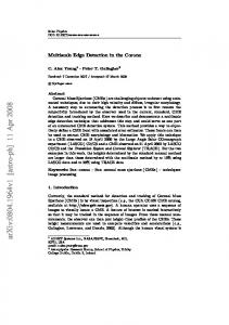
Figure 1. Electron microscope images: demonstrating the challenge of detecting edges (at different scales) embedded in noise.

Figure 2. Two adjacent noisy intensity profiles (right) parallel to a long edge (left) in an image acquired by an electron microscope.

The images in Figure 1, acquired by an electron microscope, exemplify this kind of challenge. Despite the noise (see profile plots in Figure 2), such low contrast edges are evident to the human eye due to their consistent appearance over lengthy curves. Accurate handling of low contrast edges is useful also in natural images, where boundaries between objects may be weak due to similar reflectance properties on both sides of an edge, shading effects, etc. This paper presents an algorithm for edge detection and fiber enhancement designed to work on both natural as well as very noisy images. Our method is based on efficient utilization of filters measuring difference of oriented means of various lengths and orientations, along with a theoretical estimation of the effect of noise on the response of such filters. In particular, we derive a scale adaptive threshold and use it to distinguish between significant real responses and responses due to noise at any length. We complement this with a recursive decision process to distinguish between re-

1. Introduction One of the most intensively studied problems in computer vision concerns with how to detect edges in images. Edges are important since they mark the locations of discontinuities in either depth, surface orientation, or reflectance. Edges and fibers constitute features that can support segmentation, denoising, recognition, matching and motion analysis tasks. Accurate detection of edges can be challenging, particularly when low contrast edges appear in the midst of noise. Research was supported in part by the European Commission Project IST2002-506766 Aim Shape, by the Institute for Futuristic Security Research and by the APNRR grant. Research was conducted at the Moross Laboratory for Vision and Motor Control at the Weizmann Institute of Science. We thank Ziv Reich and Eyal Shimoni for the electron microscopy images. We thank Michael Fainzilber and Ida Rishal for the light microscopy images.

1

sponses due to consistent, long edges and responses due to several scattered sub-edges. These enable us to considerably reduce the effect of noise without relying on a prior step of isotropic smoothing, and consequently reveal and accurately localize very noisy, low-contrast edges. Moreover, short gaps can be overcome, and despite the use of long filters the ”correct” ends of an edge can be delineated due to the scale multiplicity. We further present an application of this algorithm to fiber detection and enhancement by employing a stochastic completion-like process from both sides of a fiber. This process is quite robust to varying fiber width and fiber branching. Our algorithm relies on a fast, bottom-up procedure, following [1], to construct all “significantly different” oriented means at all locations, lengths, and orientations. By this, our method utilizes the same number of filters at every length, so that as we increase the length of the filter we reduce its spatial resolution and proportionally increase its directional resolution. This, along with our recursive decision process, yield efficient runtime complexity of O(N log ρ), where N is the number of pixels and ρ is the√ length of the longest structure of interest, typically ρ ≤ O( N ). Experimental results on various images are presented.

2. Previous work Common algorithms for edge detection (e.g., [3]) overcome noise by applying a preprocessing step of smoothing, typically using a gaussian kernel of a user specified width. Scale-space representations extend this approach, allowing for a simultaneous delineation of edges from all scales by combining spatially varying gaussian smoothing with automatic scale selection [10, 18]. Such isotropic smoothing, however, often reduces the contrast of weak edges, may blend adjacent edges, and may result in poor localization of edges. To avoid the pitfalls of isotropic smoothing, anisotropic diffusion schemes [15, 19, 9] were proposed as a means for edge-preserving smoothing and image enhancement. These methods utilize a diffusion tensor designed to avoid smoothing in the direction of the intensity gradients, while allowing smoothing in coherence directions. These approaches improve edge localization considerably, and edges at different scales are revealed at different iterations of the diffusion process. These edges remain visible in their original location for many iterations before they finally fade out. A scale selection mechanism however is required to extract edges of different scales. As the reliance on local gradients in traditional diffusion processes may lead to accumulation of noise, recent methods [19, 9] modify the diffusion tensor through isotropic spatial averaging or resetting of its eigenvalues. Such spatial smoothing and eigenvalue modifications are, however, adapted to a single scale. Moreover, by using an averaged diffusion tensor, these methods accumu-

late squared local intensity differences, and this may lead to smoothing across noisy, low contrast edges. The reliance on local gradients is a common problem also in both single and multiscale variational methods [14, 2]. Another stream of work utilizes filters of various lengths, widths, and orientation, yielding curvelet and contourlet image decomposition [17, 4, 7]. The focus of these methods, however, is mainly on achieving sparse representations of images and not on edge extraction or fiber enhancement. Finally, recent methods for edge detection in natural images [16, 11] compare histograms of intensity, color (and also texture in [11]) in two half disks on either sides of an edge, while in [16] the size of the disc is related to the length of the edges. While this approach avoids smoothing across a measured edge, the use of large discs may lead to smoothing across nearby edges. Furthermore, the histograms are calculated at all locations and orientations leading to inefficient schemes. Our decision process can be related to the logical-linear application proposed in [6].

3. Multiscale edge detection algorithm Our goal is to simultaneously extract edges of all lengths, in both natural and noisy images. Let I(x, y) denote a continuous function representing image intensities given in a two-dimensional domain. We denote by oriented means the family of averages of I(x, y) along rectangular patches of a given center location x = (x, y), length L, width w, and orientation θ. Typically in our implementation w is set to a small constant, yielding elongated oriented means. The family of oriented means can be obtained via integrals of the form Z w/2 Z L/2 1 F (x, L, w, θ) = (1) wL −w/2 −L/2 I(x + γ cos θ − δ sin θ, y + γ sin θ + δ cos θ)dγdδ. Our approach utilizes responses of differences of oriented means (briefly denoted responses). This family of responses is defined as 1 s w F (x + (− sin θ, cos θ), L, , θ) 2 2 2 1 s w − F (x − (− sin θ, cos θ), L, , θ), (2) 2 2 2 D(x, L, w, s, θ) =

with s ≥ w/2 to avoid overlap. D defines an average difference of neighboring oriented means of the same orientation. Given a collection of responses, our first task (Section 3.1) is to determine which response is significant. This is achieved by applying a scale adaptive threshold determined by measuring the magnitude of the noise in the image and by considering the length and width of the measured response. Next (Sec. 3.2) we examine the set of significant responses at each length. While some of these responses may

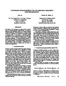
indeed indicate the presence of an edge of the appropriate length, others may be due to scattered collections of shorter edges. We therefore apply a recursive decision process to distinguish between these two cases . Finally, our algorithm relies on a framework and a data structure for efficient computation of oriented means [1] (Sec. 3.3). Figure 3. Scale-adaptive noise estimation: length-L vs. the ratio between the scale-adaptive threshold and σ.

3.1. Multiscale noise estimation Our first task is to identify differences of oriented means that elicit significant responses. In this section we derive a scale adaptive threshold that takes into account the properties of the noise as well as the length and width of our filter. Below we assume that the noise does not vary significantly across the image and that the pixel noise is normally distributed as N (0, σ 2 ). Suppose we apply differences of oriented means D(x, L, w, s, θ) to an image composed of white noise. Denote by DL,w the discrete form of D(x, L, w, s, θ), so DL,w is the average difference of two averages of wL/2 normal distributions. Consequently, DL,w itself distributes nor2 2 mally, DL,w ∼ N (0, σL ), where σL = σ 2 /(wL). In order to differentiate between responses due to realedges and those that are due to noise, we wish to estimate the chance that given a real number t À σL , a value d drawn 2 from the distribution DL,w ∼ N (0, |d| < t, ´ ³ σL )2 satisfies R t 1 x √ i.e., p(|d| < t) = 2πσ −t exp − 2σ2 dx. Therefore, L L we first estimate the following integral for t À σL µ ¶ Z ∞ Z ∞ x2 −(t + x)2 exp(− 2 )dx = exp − dx 2 2σL 2σL t 0 µ 2¶Z ∞ µ ¶ −t 2tx + x2 = exp exp − dx (3) 2 2σ 2 2σL 0 µ L2 ¶ Z ∞ µ ¶ µ ¶ 2 −t tx σL −t2 ≈ exp exp − dx = exp . 2 2 2 2σL σL t 2σL 0 With this estimate, we obtain r 2 σL t2 . p(|d| < t) ≈ 1 − exp(− 2 ) = 1 − ². π t 2σL

which means that a response which exceeds t(L, w, N ) can potentially indicate the existence of a real edge. This is the scale-adaptive threshold that we have used throughout our experiments. Clearly, it can be very useful only if we are able estimate σ, the standard deviation of the pixel noise. We suggest to estimate σ in the following simple way: for each pixel we calculate the minimal standard deviation obtained from the collection of 3 × 3 windows containing the pixel. We then construct a histogram summarizing the empirical distribution of this minimal standard deviation obtained for all the pixels. σ is determined as the 90th percentile value of this histogram. We have further confirmed this adaptive threshold empirically. We generated synthetic white noise images (200 × 200 pixels) with different values of standard deviation σ, and measured for a width w = 4 the maximal response over all length-L responses, for L = 2, 4, 8, 16, 32, 64. Figure 3 shows that the ratio obtained between the maximal response and σ qis comparable to the theoretical estimate of the ratio, i.e.,

(4)

Suppose we produce O(N ) responses of length L, where N is the number of pixels in the image. To differentiate between true edge responses and noise responses, we would like to determine an adaptive threshold t(w, L, N ) such that with high probability the values of all noise responses d obtained for a noise image will fall in the range [−t, t]. According to (4), this means (1 − ²)N = O(1), which implies 1 − ²N = O(1), in other words to assure high-probability 1 we demand 1 − ²N ≥ 1/2 or ² TL , requiring every portion of an edge to exceed its respective threshold would amount to requiring the complete length-L edge to exceed the higher threshold TcL , making the scale-adaptive threshold useless. A more relaxed approach is to require each sub-edge of length cL to pass the threshold for the complete edge TL . This approach too is unsatisfactory since, due to noise, short portions of a long edge may fall below the threshold. We address this problem by requiring that most of the sub-edges will pass some lower threshold and that the remaining gaps will be short relative to the length of the edge. We therefore define two parameters, α and β (0 ≤ α, β ≤ 1). We set αTL to be a low threshold for length-L responses. Namely, responses of length L that exceed αTL and do not exceed TL are considered nearly significant, i.e., they are not significant enough to form an edge on their own, but they can form sub-portions of longer edges. In addition, we set βL to be a threshold on the total gap size for length-L edges, i.e., a length-L edge cannot be considered significant if it contains sub-portions of total length > βL that do not exceed their respective low threshold. With such a long gap the response cannot be marked as an edge even if it exceeds its corresponding threshold TL . We implement these principles in a recursive procedure as follows. We set w and s to constants and begin with the set of responses D(x, L, w, s, θ) obtained for filters of some predetermined short length, e.g., L = 1. We classify each response to one of the following three classes: (1) significant (D > TL ) (2) nearly-significant (αTL < D ≤ TL ) and (3) non-significant (D ≤ αTL ). For the first two classes the total gap size is set to “0”, while for the latter the gap size is set to “L”. We proceed by sequentially considering lengths of powers of 2. The classification of every length-L response at location x, D(x, L, w, s, θ), is affected by the classification of its associated length-L/2 responses, D(x ± (L/4)(cos θ, sin θ), L/2, w, s, θ) as described below. In addition, the total gap size is set to be the sum of gap sizes associated with these responses. • A length-L response D is classified significant if it exceeds the respective threshold, D > TL , and its total gap size is below βL. In this case the response is marked as a potential edge and its gap size is reset to zero. • A length-L response D is classified nearly-significant if αTL < D ≤ TL and its total gap size is below βL. In this case, its gap size is not updated. • A length-L response D is classified non-significant if D ≤ αTL or if its total gap size exceeds βL. In this case its total gap size is reset to L.

Marked potential edges are further tested for statistical significance. We consider the intensity profiles along the two sides of a potential edge and denote by σlocal the maximum of the two empirical standard deviations qon either side. We ln N then remove edges for which D < c 2 wL σlocal , typically c = 1. This condition generalizes (6) by replacing the global noise σ with a local estimate of the noise, σlocal , yielding a scale-dependent local threshold. This test allows us to be less strict with the selection of α and β. Finally, we apply a process of angular non-maximal suppression followed by spatial non-maximal suppression at each length L. The non-maximal suppression is a necessary step to ensure well-localized edges, expressed by a single response. Moreover, we perform an inter-scale suppression, to ensure that each edge is identified with its maximal perceptual length. This inter- and intra-scale decision process along with the scale-adaptive threshold allow us to overcome noise without prior smoothing, and therefore to reveal and accurately localize very noisy, low-contrast edges.

3.3. Hierarchical construction of oriented means We construct our differences of oriented means by adding and subtracting width-1 oriented means of the appropriate length. The family of width-1 oriented means, F (x, L, w, θ) is defined over an infinite set of locations, lengths, and orientations, but under minimal smoothness assumptions of I(x, y) it is possible to obtain any oriented mean in this family from only a finite collection of oriented means. Oriented means at interim locations, lengths, and orientations can then be computed by interpolation with an accuracy determined by the spatial and angular resolutions. Following [1], the minimal spatial and angular resolutions depend on the length L as follows. • The minimal spatial resolution in the direction of integration is inversely proportional to the integration length. In particular, when doubling the integration length, the number of evaluation points may be halved. • The spatial resolution perpendicular to the direction of integration is independent of the integration length. • The minimal angular resolution is proportional to the integration length. In particular, if the integration length is doubled, the number of angles computed per site must also be doubled. A direct consequence of these observations is that the total number of integrals at any length L is independent of L. Figure 4(left) depicts the common direct approach to approximating discrete oriented means of orientation |θ| ≤ π4 . Using the trapezoid rule, the oriented mean for, e.g., the line segment depicted in Figure 4(left), is given by the

Figure 4. Left panel: Direct calculation of oriented mean (w = 1, L = 4): an interpolation from the given data points to the red points is followed by the trapezoid rule. Right panel: Base level initialization: stencil of four length-1 integrals for each pixel (left) cover the whole grid (right).

sum over the three interior points (obtained by interpolation from nearby data points) plus the average of the endpoints, divided by four. Similar calculation applies for oriented means with π4 ≤ θ ≤ 3π 4 . However, this direct approach is quite expensive to approximate many oriented means. In the remainder of this section we follow [1] and describe a fast, hierarchical recursive calculation of “all significantly different” oriented means in a discrete image. In the context of a discrete image, we define the length of an oriented mean on a uniform grid as the length of its maximal projection onto the x- and y-axis, where the length units are pixels. The hierarchical construction is as follows. At the base level, for each pixel four length-1 oriented means are calculated (see Figure 4(right)). The total number of oriented means at this level is therefore 4N . Recursively, given 4N oriented means of length L we proceed to computing new 4N oriented means of length 2L. Following the principles outlined above, the angular resolution should be doubled. Consequently, the new oriented means can be divided into two equally sized sets. Half of the new oriented means follow the same directions of those of the previous level, while the other half of the oriented means follow intermediate directions. The first set of oriented means can be computed simply by taking the average of two, length-L oriented means with one coinciding endpoint (see Figure 5, left panel). The second set of oriented means can be obtained by interpolation of four length-L oriented means of nearby directions. These four oriented means form a tight parallelogram around the desired length-2L integral. This is illustrated in Figure 5 (left panel), where the average of the four length-1 oriented means is used to construct a length-2 oriented mean. This can be viewed as first linearly interpolating the two nearest directions to approximate the new direction at length-1, then creating a length-2 oriented mean by averaging two adjacent interpolated oriented means. It should be emphasized that the numerical error introduced by this fast calculation, relative to the slow, direct approach, is smaller than the error induced by discretizing I(x, y). The algorithm is very efficient, it calculates “all significantly different” oriented means in O(N log ρ), where N is the number of pixels in the image and ρ √ is the length of the longest oriented mean, typically ρ ≤ O( N ).

Figure 5. Left panel: Building integrals of length-2 from integrals of length-1, for existing directions (left), by taking the average of length-1 adjacent integrals (dashed lines) in that direction, and for a new direction (right), by averaging four nearest integrals (dashed lines). Right panel: The red lines denote length-4 vertically oriented means, which are calculated at each 2nd row (pink rows). The blue lines denote length-4 horizontally oriented means, which are calculated at each 2nd column (blueish columns).

3.4. Implementation For our implementation we maintain a hierarchical data structure of the angular and spatial resolutions as follows. At the base level, for each pixel length-1 oriented means at four directions are calculated. The angular resolution of length-2L oriented means is twice the angular resolution of length-L oriented means. The spatial resolution is halved as the length is doubled as follows. Length-L vertically orith ented means ( π4 ≤ θ ≤ 3π 4 ) are calculated at every (L/2) row, at each pixel in this row. Length-L horizontally oriented means (|θ ≤ π4 |) are calculated at every (L/2)th column, at each pixel in this column. In this manner, each length-L oriented mean has an overlap of length L/2 with another length-L oriented mean of the same orientation, in order to improve accuracy. As a result, at each scale (length) the number of oriented means is 8N , except for the shortest level (length-1) for which 4N oriented means are calculated. Note that at each length only 4N of the 8N oriented means are used to construct the subsequent level. The grid setting for L = 4 is illustrated in Figure 5(right). Our recursive decision process is evoked during the construction of oriented means after the construction of every length, maintaining the low complexity of the algorithm. For this decision process we associate with each length-L response the two (if the longer response follows an orientation of the previous level) or four (if the longer response is of a “new” orientation) length-L/2 responses from which it was generated. Finally, the local standard deviation test can be applied by accessing the raw pixels, assuming only a sparse set of responses are considered significant. Alternatively, σlocal can be recursively accumulated by computing in addition oriented means for the squared intensities, I 2 (x, y), doubling the overall complexity.

4. Experiments Our algorithm employs differences of oriented means D(x, L, w, s, θ) at lengths L = 1, 2, 4, 8, 16, 32, 64, with s = 2, w = 2 and s = 5, w = 4 for the edge detection in

natural images and noisy images, respectively.

4.1. Noisy images We have implemented our edge detection algorithm and tested it on very noisy images acquired by electron √ microscope. For this implementation we use α = 0.5 and β = 3/8. Figure 6 contains images of a plant under certain photosynthetic conditions. Depending on lighting, the membranes, which are sub-cell organs (organelles), are sometimes very close to each other. As demonstrated in the figure, our algorithm performs very well in detecting the edges of the membranes, independently of the scale (length) and the membranes’ density (Figure 6, middle row). Canny edge detector (with optimized parameters) cannot reveal these dense edges, due to the pre-smoothing (Figure 6, bottom row). We compare our algorithm with our own implementation (following [8]) of the Beltrami flow anisotropicdiffusion. The enhanced images and their respective inverse gradients are shown in Figure 7. It can be seen that different structures are enhanced in different iterations, yet the dense organelles structure is not revealed at any iteration, and the overall result is severely affected by the amount of noise present in this image. Figure 8 contains images of bacteria environment. Our algorithm extracts edges at all scales, both elongated and circular.

4.2. Natural images We have further applied our algorithm to the 100 gray level test images of the Berkeley segmentation dataset and human annotation√benchmark [12]. For this implementation we use α = 0.8 and β = 0. Although this dataset is not ideal for evaluating our method as (1) human annotation is affected to a large extent by semantic considerations, (2) subjects only marked subsets of the boundaries, and (3) our method does not deal with texture; it nevertheless demonstrates that our method achieves competitive results on natural images. To determine boundary classification we associate a response with every edge point in a manner similar to that used in [11]. Specifically, we compute two intensity histograms for the two half-discs (using discs of radius 7 pixels) centered in each edge center and oriented according to the edge direction. We then use a χ2 histogram difference measure to compare the two hisP (gi −hi )2 tograms χ2 (g, h) = 12 gi +hi . We finally normalize these values (for each image) between 0 and 1. Figure 9 shows some example images, demonstrating the exact localization of edges that can be achieved with our method. We further used the standard F-measure test, which provides a trade-off between precision (P ) and recall (R) defined as F = P R/(γR + (1 − γ)P ), with γ set to 0.5. These are computed using a distance tolerance of 2 pixels to allow for small localization errors in both the machine and

Figure 6. Edge detection. Top row: original images. Middle row: edges obtained by algorithm overlaid on the original images. Bottom row: edges obtained by Canny edge detector.

Figure 7. Image enhancement and inverse gradient by Beltrami flow. Top row: image enhancement after 8, 11 and 20 iterations, respectively (from left to right). Bottom row: respective inverse gradients.

human boundary maps. Table 1 shows the F-measure values achieved by our algorithm compared to other edge detection algorithms. Note that somewhat better performance

This process is analogous to stochastic completion of contours [13] with each edge point emitting particles to its surroundings. The product of the diffusion maps reflects the probability of beginning in one edge and ending in a neighboring edge of opposite gradient sign. This process is quite robust to varying fiber width and fiber branching, and although many red and blue responses may appear in the image, only those that can be paired are enhanced.

Figure 8. Edge detection. Left column: original images. Right column: edges obtained by our algorithm overlaid on the original images.

is achieved by methods that use color and texture features such as [11]. Code and results of other algorithms are obtained from Berkeley at http://www.eecs.berkeley.edu/Research/Projects/ CS/vision/grouping/segbench/. Algorithm

F-measure

We applied our fiber enhancement process to fluorescent images of nerve cells. Comparison of these cells under different conditions requires quantitative measurements of cellular morphology, and a commonly used measure is the total axonal length. Typically, a single experiment produces hundreds of images, many of which may suffer from low signal to noise ratio. Therefore, there is an obvious need for fast and accurate automatic processing of such images. Using our multiscale fiber enhancement method we identify the branching axonal structures and measure their total length. Figure 10 shows examples of images of nerve cells and their enhanced axonal structures. The total axonal length was further computed automatically from the enhanced images and compared to a manual length estimation applied to the original images. The two measures match with slight devia√ tion, see Table 2. For this implementation we use α = 0.5 and β = 0.0.

our multiscale edge detection algorithm

0.61

Brightness Gradient

0.60

Multiscale Gradient Magnitude

0.58

Second Moment Matrix

0.57

Gradient Magnitude

0.56

Manual estimation

11940

4467

3407

0.41

Automatic estimation

11180

4106

3620

9092

Relative error (percents)

-6.37

-8.08

6.25

23.75

Random

Table 1. F-measure comparison over edge detection algorithms.

Our non-optimized (combined Matlab and C++) implementation requires 3, 11, and 18 seconds for 171 × 246, 481 × 321, and 512 × 512 images respectively on a Pentium 4, 2.13GHz PC.

7347

Table 2. Measuring total axonal length: manual length estimation vs. automatic length estimation (in pixel units), for the four leftmost images in Figure 10.

5. Fiber detection and enhancement

6. Conclusion

Our method is further extended to detect and enhance elongated fibers. Fibers appear in many types of images, particularly in biomedical imagery and airborne data. Detection of fibers can be difficult due to both imaging conditions (noise, illumination gradients) and shape variations (changes in widths, branchings). We propose a method that uses edges, along with their sign (transition from dark to light or vice versa) to highlight the fibers. Specifically, we begin by detecting all edges in the image. We next mark those edges as either “red” or “blue”, by classifying their gradient orientation relative to a pre-specified canonical orientation. We then construct two diffusion maps, one for the red and the other for the blue edge maps, by convolving the binary edge map with a gaussian filter. Finally, we multiply the two diffusion maps to obtain the enhanced fibers.

We have presented an algorithm for edge detection suitable for both natural as well as noisy images. Our method utilizes efficient multiscale hierarchy of responses measuring the difference of oriented means of various lengths and orientations. We use a scale-adaptive threshold along with a recursive decision process to reveal the significant edges at all scales and orientations and to localize them accurately. We have further presented an application to fiber detection and enhancement by utilizing stochastic completionlike process from both sides of a fiber. Our current method identifies curved edges as concatenation of short straight responses. We plan to construct a direct framework to detect curved edges. We further plan to extend our algorithm to handle edges of varying widths and to estimate and incorporate local noise.

Figure 9. Edge detection results. Top: original images. Middle: our results. Bottom: human-marked boundaries.

Figure 10. Neuron enhancement results. Top: original images acquired by light microscope. Bottom: enhanced neurons.

References [1] A. Brandt and J. Dym. Fast calculation of multiple line integrals. SIAM, JSC, 20(4):1417–1429, 1999. 2, 3, 4, 5 [2] X. Bresson, P. Vandergheynst, and J. Thiran. Multiscale active contours. IJCV, 70(3):197–211, 2006. 2 [3] J. Canny. A computational approach to edge detection. TPAMI, 8:679–698, 1986. 2 [4] M. Do and M. Vetterli. The contourlet transform: an efficient directional multiresolution image representation. IEEE, Trans. on Image Processing, 14(12):2091–2106, 2005. 2 [5] A. Frangi, W. Niessen, K. Vincken, and M. Viergever. Multiscale vessel enhancement filtering. LNCS, 1496:130–137, 1998. [6] L. A. Iverson and S. W. Zucker. Logical/linear operators for image curves. IEEE Transactions on Pattern Analysis and Machine Intelligence, 17(10):982–996, 1995. 2 [7] S. Kalitzin, B. T. H. Romeny, and M. Vierger. Invertible apertured orientation filters in image analysis. IJCV, 31(2), 1999. 2 [8] R. Kimmel, M. Bronstein, and A. Bronstein. In Numerical geometry of images: Theory, algorithms and applications, page 148. SpringerVerlag, New York, 2004. 6 [9] R. Kimmel, R. Malladi, and N. Sochen. Images as embedded maps and minimal surfaces: Movies, color, texture, and volumetric medical images. IJCV, 39:111–129, 2000. 2 [10] T. Lindeberg. Edge detection and ridge detection with automatic scale selection. CVPR, page 465, 1996. 2

[11] D. Martin, C. Fowlkes, and J. Malik. Learning to detect natural image boundaries using local brightness, color, and texture cues. TPAMI, 26(5):530–548, 2004. 2, 6, 7 [12] D. Martin, C. Fowlkes, D. Tal, and J. Malik. A database of human segmented natural images and its applications to evaluating segmentation algorithms and measuring ecological statistics. ICCV, 2:416– 423, 2001. 6 [13] D. Mumford. Elastica and computer vision. In C. Bajaj, editor, Algebraic geometry and its applications. Springer, 1994. 7 [14] D. Mumford and J. Shah. Optimal approximation by piecewise smooth functions and associated variational problems. Comm. on Pure Applied Math., 42:577–685, 1989. 2 [15] P. Perona and J. Malik. Scale space and edge detection using anisotropic diffusion. TPAMI, 12(7):629–639, 1990. 2 [16] M. Ruzon and C. Tomasi. Edge, junction, and corner detection using color distributions. TPAMI, 23(11):1281–1295, 2001. 2 [17] J. Starck, F. Murtagh, E. Cand`es, and D. Donoho. Gray and color image contrast enhancement by the curvelet transform. IEEE, Trans. on Image Processing, 12(6):706–717, 2003. 2 [18] M. Tabb and N. Ahuja. Multiscale image segmentation by integrated edge and region detection. IEEE, Trans. on Image Processing, 6(5):642–655, 1997. 2 [19] J. Weickert. A review of nonlinear diffusion filtering. Scale-Space Theory in Computer Vision, LNCS, 1252:3–28, 1997. 2