Multiscale inference for multivariate deconvolution arXiv:1611.05201v1

Multiscale inference for multivariate deconvolution Konstantin Eckle, Nicolai Bissantz, Holger Dette Ruhr-Universit¨at Bochum

arXiv:1611.05201v1 [stat.ME] 16 Nov 2016

Fakult¨at f¨ ur Mathematik 44780 Bochum, Germany

Abstract In this paper we provide new methodology for inference of the geometric features of a multivariate density in deconvolution. Our approach is based on multiscale tests to detect significant directional derivatives of the unknown density at arbitrary points in arbitrary directions. The multiscale method is used to identify regions of monotonicity and to construct a general procedure for the detection of modes of the multivariate density. Moreover, as an important application a significance test for the presence of a local maximum at a pre-specified point is proposed. The performance of the new methods is investigated from a theoretical point of view and the finite sample properties are illustrated by means of a small simulation study.

Keywords and Phrases: deconvolution, modes, multivariate density, multiple tests, Gaussian approximation AMS Subject Classification: 62G07, 62G10, 62G20

1

Introduction

In many applications such as in biological, medical imaging or signal detection only indirect observations are available for statistical inference, and these problems are called inverse problems in the (statistical) literature. In the case of medical imaging, a well-known example is Positron Emission Tomography. Here, the connection between the ’true’ image and the observations involves the Radon transform [see, for example, Cavalier (2000)]. Other typical examples are the reconstruction of biological or astronomical images, where the connection between the true image and the observable image is - at least in a first approximation - given by convolution-type operators [see, for example, Adorf (1995) or Bertero et al. (2009)]. Whereas in these models the data is in general described in a regression framework, similar (de-)convolution problems arise 1

in density estimation from indirect observations [see Diggle and Hall (1993) for an early reference]. The corresponding (multivariate) statistical model for density deconvolution is defined by Yi = Zi + εi , i = 1, . . . , n, (1.1) where (Z1 , ε1 ), . . . , (Zn , εn ) ∈ Rd × Rd are independent identically distributed random variables and the noise terms ε1 , . . . , εn are are also independent the of the random variables Z1 , . . . , Zn . We assume that the density fε of the errors εi is known and are interested in properties of the density f of the random variables Zi based on the sample {Y1 , . . . , Yn }. In terms of densities, model (1.1) can be rewritten as g = f ∗ fε , where g denotes the density of Y1 . Density estimators can be constructed and investigated similarly to the regression case (see the references in the next paragraph), and in this paper we are interested in describing qualitative features of the density f using the sample {Y1 , . . . , Yn }. In particular we will develop a method for simultaneous detection of regions of monotonicity of the density f at a controlled level and construct a procedure for the detection of the modes of f . To our best knowledge multivariate problems of this type have not been investigated so far in the literature. On the other hand there exists a wide range of literature concerning statistical inference in the univariate deconvolution model. A Fourier-based estimate of the density f using a damping factor for large frequencies was introduced in Diggle and Hall (1993), whereas Pensky and Vidakovic (1999) estimate f with a wavelet-based deconvolution density estimator [see also van Es et al. (1998) for a nonparametric estimator for the corresponding distribution function or Butucea and Matias (2005) for a plug-in estimator of f based on estimation of a scale parameter for the noise level]. Bissantz et al. (2007) develop confidence bands for deconvolution kernel density estimators, while minimax rates for this estimation problem can be found in Carroll and Hall (1988) and Fan (1991). Romano (1988) and Grund and Hall (1995) point out that the detection of regions of monotonicity and of the modes of a density is a more complex problem and Fan (1991) shows that the minimax rate for estimating the derivative over a H¨older-β-class (β ≥ 2) in the univariate setting d = 1 is given by n−(β−1)/(2β+2r+1) , where r > 0 denotes the order of polynomial decay of the Fourier transform of the error density fε . Balabdaoui et al. (2010) develop a test for the number of modes of a univariate density and Meister (2009) proposes a local test for monotonicity for a fixed interval. More recently Schmidt-Hieber et al. (2013) discuss multiscale tests for qualitative features of a univariate density which provide uniform confidence statements about shape constraints such as local monotonicity properties. Little research has been done regarding multivariate deconvolution problems. Recent references for density estimation are e.g. Comte and Lacour (2013) using kernel density estimators and Sarkar et al. (2015) for a Bayesian approach in the case of an unknown error distribution with 2

replicated proxies available. Hypothesis testing in deconvolution is investigated in Holzmann et al. (2007) and Bissantz and Holzmann (2008). In the present paper we will develop a multiscale method for simultaneous identification of regions of monotonicity of the multivariate density f in the deconvolution model (1.1). Our approach is based on simultaneous local tests of the directional derivatives of the density f for a significant deviation from zero for “various” directions and locations. In Section 2 we present a Fourier based method for the construction of local tests, which will be used for the inference about the monotonicity properties of the density f . Roughly speaking, we propose a multiscale test investigating the sign of the derivatives of the density f in different locations and directions and on different scales. Section 3 is devoted to asymptotic properties, which can be used to obtain a multiscale test for simultaneous confidence statements about the density. Moreover, we also propose a method for the detection and localization of the modes. The finite sample properties of the method are discussed in Section 4 and all proofs are deferred to Sections 5 and 6, while Section 7 contains two technical results.

2

Multiscale inference in multivariate deconvolution

Let ∂s denote the directional derivative in the direction of s ∈ S d−1 = {s ∈ Rd | ksk = 1} and φ : Rd → R≥0 be a sufficiently smooth kernel (i.e. kφkL1 (Rd ) = 1) with compact support in [−1, 1]d . Define
for t ∈ [0, 1]d , h > 0. φt,h (.) = h−d φ .−t h For the description of the local monotonicity properties of the function f we introduce the integral Z − ∂s f (x)φt,h (x) dx. (2.1) Rd

If this expression is, say, negative, we can conclude that the derivative of f in direction s has to be strictly larger than zero on a subset of positive Lebesgue measure of the cube [t1 − h, t1 + h] × . . . × [td − h, td + h]. Statistical inference regarding the monotonicity properties of f can then be performed by testing simultaneously several hypotheses of the form Z Z sj ,tj ,hj sj ,tj ,hj H0,incr : − ∂sj f (x)φtj ,hj (x) dx ≥ 0 versus H1,incr : − ∂sj f (x)φtj ,hj (x) dx < 0 (2.2) Rd

Rd

and sj ,tj ,h H0,decr j

Z :− Rd

∂sj f (x)φtj ,hj (x) dx ≤ 0 versus

sj ,tj ,h H1,decr j

Z :− Rd

∂sj f (x)φtj ,hj (x) dx > 0 , (2.3)

where (s1 , t1 , h1 ), . . . , (sp , tp , hp ) are given triples of directions, locations and scaling factors. 3

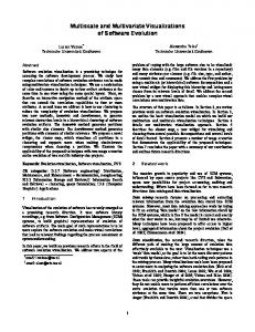
Figure 1: Example of a global map for monotonicity of a bivariate density. This method allows for a global understanding of the shape of the density f . A particular feature of the proposed method consists in the fact that by conducting formal statistical tests the multiple level can be controlled (see Theorem 3.2). For example, simultaneous tests for hypotheses of the form (2.2) and (2.3) can be used to obtain a graphical representation of the local monotonicity behavior of the density as displayed in Figure 1 for a bivariate density. The displayed map is based on tests for the hypotheses (2.2) for a fixed scale h0 and different locations and directions (s1 , t1 ), . . . , (sp , tp ) (here taken as the vertices of an equidistant grid and four equidistant directions on S 1 ). Note that we are investigating here a symmetric set of triples, that is, for every location tj both the triple sj ,tj ,h0 −sj ,tj ,h0 (sj , tj , h0 ) and (−sj , tj , h0 ) are considered. Thus, as H0,incr = H0,decr , it is sufficient to investigate only hypotheses of the form (2.2) in this setting. The figure shows the results of the tests for the different hypotheses in (2.2). An arrow in a direction sj at a location tj represents sj ,tj ,h0 a rejection of the corresponding hypothesis H0,incr and provides therefore an indication of a j positive directional derivative of f in direction s at the location tj . For a detailed description of the settings used to provide Figure 1 and an analysis of the results we refer to Section 4.2. If one is interested in specific shape constraints of the density, say in a test for a mode (local maximum) at a given point x0 , inference can be conducted investigating the hypotheses j

j

s ,t ,h0 H0,decr

j

j

s ,t ,h0 versus H1,decr

(2.4)

for different pairs (t1 , s1 ), . . . , (tp , sp ), where t1 , . . . , tp are points in a neighborhood of x0 on the lines {x0 + λsj |λ > 0} (j = 1, . . . , p), respectively (of course, on could additionally use different scales here).

4

Throughout this paper we will assume that all partial derivatives ∂s f of the density f are uniformly bounded, such that the estimated quantity (2.1) is bounded by a constant which does not depend on the triple (s, t, h). Using integration by parts, Plancherel’s identity and the convolution theorem, we get Z Z − ∂s f (x)φt,h (x) dx = f (x)∂s φt,h (x) dx (2.5) Rd Rd Z 1 = F (f )(y)F (∂s φt,h )(y) dy (2π)d Rd   Z F (∂s φt,h ) 1 = F (g)(y) (y) dy (2π)d Rd F (fε )   Z −1 F (∂s φt,h ) = g(x)F (x) dx. F (fε ) Rd Here, F (f )(y) =

Z

e−iy.x f (x) dx, Z 1 −1 F (f )(x) = eix.y f (y) dy (2π)d Rd Rd

x, y ∈ Rd




denote the Fourier transform and its inverse, respectively, z is the complex conjugate of z ∈ C and x.y stands for the standard inner product of x, y ∈ Rd . For the construction of tests for the hypotheses in (2.2) and (2.3) we define the statistic n

n Ts,t,h

1X = Fs,t,h (Yi ), n i=1

where Fs,t,h (Yi ) = F

−1

 F (∂ φ )  s t,h F (fε )

(2.6)

(Yi ).

(2.7)

Because (by (2.5)) n ) E(Ts,t,h

Z =−

∂s f (x)φt,h (x) dx, Rd

n it follows that Ts,t,h is a reasonable estimate of the quantity defined in (2.1), and hence the n statistics Ts,t,h define the main tool to study qualitative features of the density f . Inference on s,t,h local monotonicity of the density f will then be based on tests rejecting the hypotheses H0,incr s,t,h n n for small values of the corresponding statistic Ts,t,h and rejecting H0,decr for large values of Ts,t,h for several directions s ∈ S d−1 , locations t ∈ [0, 1]d and scales h > 0. The multiple level of these tests can be controlled by investigating the (asymptotic) maximum of appropriately normalized n statistics Ts,t,h calculated over a certain set of locations, directions and scales.

5

3

Asymptotic properties

In this section we investigate the asymptotic properties of a statistic which can be used to control the multiple level of the tests introduced in Section 2. To be precise, we consider the finite subset  Tn := (sj , tj , hj ) | j = 1, . . . , p ⊆ S d−1 × [0, 1]d × [h min , h max ] of cardinality p ≤ nK for the calculation of the maximum of appropriately standardized statistics n Ts,t,h , where K > 1 and for some ε > 0 h min & n−1/d+ε and h max = o((log(n) log log(n))−1 ).

(3.1)

Throughout this paper we will make frequent use of multi-index notation, where α = (α1 , . . . , αd ) ∈ Nd0 denotes a multi-index (written in bold), |α| = α1 + . . . + αd its “length”, and for a sufficiently smooth function f : Rd → R and a multi-index α we denote by ∂ α f (x) =

∂xα1 1

∂ |α| f (x) · . . . · ∂xαd d

its partial derivative. Recall the definition of Fs,t,h in (2.7), to simplify the notation define for a point (sj , tj , hj ) ∈ Tn (3.2)

Fj = Fsj ,tj ,hj and consider the random variables q n q  hd/2+r+1 X  log(eh−d j ) j (1) −d ˜ p F (Y ) − nE(F (Y )) − Xj = 2 log(h ) , j i j 1 j log log(ee h−d nˆ gn (tj )Vj i=1 j )

(3.3)

where gˆn is a density estimator of g satisfying kg − gˆn k∞ = o(log(n)−1 ) almost surely

(3.4)

(for example a kernel density estimator as considered in Gin´e and Guillou (2002)) and d/2+r+1

Vj = hj

kFsj ,tj ,hj kL2 (Rd ) .

(3.5)

The quantity Vj is well-defined under the assumptions presented below (see Lemma 5.2 for details). sj ,tj ,h sj ,tj ,h Note that the boundary of the hypotheses H0,incr j and H0,decr j in (2.2) and (2.3) is defined by R ∂ j f (x)φtj ,hj (x) dx = 0 and in this case we have Rd s q q −d  d/2+r+1  log(eh ) 2 log(h−d hj j j ) 1 ˜ (1) n √ Xj = p √ T − . j j s ,t ,hj n n log log(ee h−d gˆn (tj )Vj j ) (1)

˜ Consequently, we will investigate the asymptotic properties of max1≤j≤p X j discussion. For this purpose we make the following assumptions. 6

in the following

Assumption 1. Assume that the density g is Lipschitz continuous and locally bounded from below, i.e. g(x) ≥ c > 0 for all x ∈ [0, 1]d . Assumption 2. We assume a polynomial decay of the Fourier transform of the error density fε , i.e. that there exist constants r > 0 for d ≥ 2 resp. r > 21 for d = 1 and 0 < Cu < Co such that
−r/2
−r/2 . ≤ |F (fε )(y)| ≤ Co 1 + kyk2 Cu 1 + kyk2 Furthermore, let d(d+1)/2e

X j=1

∂j j F (fε )(y) ≤ Co (1 + kyk2 )−r/2 ∂yl

2 j/2

(1 + kyk )

for all l = 1, . . . , d. Note that as a direct consequence of Assumption 1 g is bounded from above and that there exists a constant δ > 0 such that g(x) ≥ 2c > 0 for all x ∈ [−δ, 1 + δ]d . Assumption 2 can be seen as a multivariate generalization of the classical assumptions on the decay of the Fourier transform of the error density in the ordinary smooth case (see e.g. Schmidt-Hieber et al. (2013), Assumption 2). We also note that this assumption defines a mildly ill-posed situation (see Bissantz and Holzmann (2008)). The next assumptions refer to the kernel φ and are required for some technical arguments. Assumption 3. Let k∂s φkL2 (Rd ) 6= 0 for all s ∈ S d−1 and assume that ∂ β φ exists in [−1, 1]d and is continuous for all |β| ≤ dr + 2e, where r is the constant from Assumption 2. We assume further that for some δ > 0 the inequality Z m 2
2 r+(d+δ)/2 ∂ 1 + kyk m F (∂ek φ)(y) dy < ∞ ∂yl Rd holds for all k, l = 1, . . . , d and m = 0, . . . , d(d + 1)/2e, where ek , k = 1, . . . , d, denotes the kth unit vector of Rd . As

d d m ∂m 2 X 2 2 X ∂m ∂ sk m F (∂ek φ)(y) ≤ C m F (∂s φ)(y) = m F (∂ek φ)(y) ∂yl ∂yl ∂yl k=1 k=1

for all s ∈ S d−1 and some constant C > 0 that only depends on d, Assumption 3 yields a uniform upper bound for the integral Z 2
r+(d+δ)/2 ∂ m 1 + kyk2 m F (∂s φ)(y) dy ∂yl Rd 7

for all s ∈ S d−1 . ˜ (1) in (3.3) and define the vector X ˜ (1) = (X ˜ 1(1) , . . . , X ˜ p(1) )> . Our Recall the definition of X j ˜ (1) ∈ A) by the first main result provides a uniform approximation of the probabilities P(X ˜ ∈ A) for every half-open hyperrectangle A, where the components of the probabilities P(X ˜ = (X ˜1, . . . , X ˜ p )> are defined by vector X q R   log(eh−d j ) | F (x) dBx | q d/2+r+1 −d Rd j ˜ hj − 2 log(hj ) (3.6) Xj = Vj log log(ee h−d j ) (j = 1, . . . , p), and (Bx )x∈Rd is a standard d-variate Brownian motion. Theorem 3.1. Let A denote the set A := {(−∞, a1 ] × . . . × (−∞, ap ] | a1 , . . . , ap ∈ R}. Then,

˜ (1) ∈ A − P X ˜ ∈ A = o(1) for n → ∞. sup P X (3.7) A∈A

˜ j is almost surely bounded uniformly with respect Furthermore, the random variable max1≤j≤p X to n. Theorem 3.1 will be used to control the multiple level of statistical tests for the hypotheses of the form (2.2) and (2.3). To this end, let α ∈ (0, 1) and denote by κn (α) the smallest number such that   ˜ P max Xj ≤ κn (α) ≥ 1 − α. (3.8) 1≤j≤p

By Theorem 3.1, κn (α) is bounded uniformly with respect to n and α. The jth hypothesis in (2.2) is rejected, whenever n X −1 n Fj (Yi ) < −κjn (α), (3.9) i=1

where κjn (α)

p q  gˆn (tj )Vj −d/2−r−1  log log(ee h−d j ) √ q hj κn (α) + 2 log(h−d ) . = j n −d log(eh )

(3.10)

j

Similarly, the jth hypothesis in (2.3) is rejected, whenever n

−1

n X

Fj (Yi ) > κjn (α).

(3.11)

i=1

Theorem 3.2. Assume that the tests (3.9) and (3.11) for the hypotheses (2.2) and (2.3) are performed simultaneously for j = 1, . . . , p. The probability of at least one false rejection of any of the tests is asymptotically at most α, that is n   X P ∃j ∈ {1, . . . , p} : n−1 | Fj (Yi )| > κjn (α) ≤ α + o(1) i=1

for n → ∞. 8

Next we introduce a method for the detection and localization of the modes of the density. The main idea is to conduct the local tests for modality proposed in (2.4) for a set of candidate modes which does not assume any prior knowledge about the density. To be precise, we assume the following condition on the set Tn : for any fixed h and s the set {t : (s, t, h) ∈ Tn } is an equidistant grid in [0, 1]d with grid width h. Furthermore, for any fixed t and h the set {s : (s, t, h) ∈ Tn } is a grid in S d−1 with grid width converging to zero with increasing sample size. 0 This grid is now used as follows to check if a point x0 ∈ (0, 1)d is a mode of f . Let Tnx ⊂ Tn be √ √ the set of all triples (s, t, h) ∈ Tn such that ch ≥ kx0 − tk ≥ 2 dh for some c > 2 d sufficiently large and angle(x0 − t, s) → 0 for n → ∞. By the condition on Tn defined above, the set 0 Tnx is nonempty for sufficiently large n. We now use the local tests (3.11) for the hypotheses (2.4) and decide for a mode at the point x0 if the null hypotheses in (2.4) are rejected for all 0 triples in Tnx . Note that by choosing the test locations as the vertices of an equidistant grid no prior knowledge about the location of x0 has to be assumed. Theorem 3.3 below states that the procedure detects all modes of the density with asymptotic probability one as n → ∞. Theorem 3.3. Let x0 ∈ (0, 1)d denote an arbitrary mode of the density f and assume that there exist functions gx0 : Rd → R, f˜x0 : R → R such that the density f has a representation of the form f (x) ≡ (1 + gx0 (x))f˜x0 (kx − x0 k) (3.12) (in a neighborhood of x0 ), gx0 is differentiable in a neighborhood of the point x0 such that gx0 (x) = o(1) and h∇gx0 (x), ei = o(kx − x0 k) if x → x0 for all e ∈ Rd with kek = 1. In addition, let f˜x0 be differentiable in a neighborhood of the point 0 with f˜x0 0 (h) ≤ −ch(1 + o(1)) for h → 0. If the set  (s, t, h) ∈ Tn : h ≥ C log(n)1/(d+2r+4) n−1/(d+2r+4) for some C > 0 sufficiently large is nonempty, then the procedure described in the previous paragraph detects the mode x0 with asymptotic probability one as n → ∞. The method to detect the modes of the density proposed in Theorem 3.3 proceeds in two steps: the verification of the presence of a mode with asymptotic probability one in the asymptotic regime presented above and its localization at the rate n−1/(d+2r+4) (up to some logarithmic factor) given by the grid width.

4

Finite sample properties

In this section we illustrate the finite sample properties of the proposed multiscale inference. The performance of the test for modality at a given point x0 (see the hypotheses in (2.4)) and 9

the dependence of its power on the bandwidth and the error variance is investigated. We also illustrate how simultaneous tests for hypotheses of the form (2.2) and (2.3) can be used to obtain a graphical representation of the local monotonicity properties of the density. We consider two-dimensional densities, i.e. d = 2. The density fε of the errors in model (1.1) is given by a symmetric bivariate Laplacian with scale parameter σ > 0 which is defined through its characteristic function 1 (4.1) F (fε )(y1 , y2 ) = 1 2 2 1 + 2 σ (y1 + y22 ) for (y1 , y2 ) ∈ R2 (cf. Kotz et al. (2001), Chapter 5). This means that r = 2 and straightforward calculations show that   
 σ2 2 F (∂s φt,h ) 2 Fs,t,h (x1 , x2 ) = F −1 F (f ∂ ∂ + ∂ ∂ φt,h (x1 , x2 ) (4.2) (x , x ) = ∂ − 1 2 s 1 2 s e s ε) 2 e for (x1 , x2 ) ∈ R2 . The test function is chosen as  φ(x1 , x2 ) = c2 (1 − x41 )(1 − x42 )1 |x1 | ≤ 1, |x2 | ≤ 1 , where c2 defines the normalization constant, that is

 −1 c2 = (1 − x41 )(1 − x42 )1 |x1 | ≤ 1, |x2 | ≤ 1 L1 (Rd ) (note that φ is smooth within its support). Moreover, the integration by parts formula gives Z Z f (x)∂s φt,h (x) dx ∂s f (x)φt,h (x) dx = − R2

R2

as φ vanishes on the boundary of its support. Finally, by the representation (4.2) we find that the deconvolution kernel possesses all properties that are used for the proof of Theorem 3.1 and therefore Theorem 3.1 is also satisfied for the function φ. Throughout this section the nominal level is fixed as α = 0.05.

4.1

A local test for modality

In this section we investigate the performance of a local test for the existence of a mode (more precisely a local maximum) at a given location x0 which is defined by testing several hypotheses of the form (2.4) simultaneously. Moreover, the influence of the choice of the different parameters on the power of the test is also investigated. To be precise, we conduct four tests for the hypotheses (2.4) with a fixed bandwidth h = h0 . The postulated mode is given by the point x0 = (0, 0)> and the four directions and locations are chosen as s1 = t1 = (1, 0)> ,

10

Figure 2: Illustration of the four local tests for monotonicity used to define the test (4.3) for h0 = 0.5. The crosshatched squares display the support of the functions Fsj ,tj ,h0 , j = 1, . . . , 4, and the arrows the directional vectors sj , j = 1, . . . , 4. s2 = t2 = (0, 1)> , s3 = t3 = (−1, 0)> and s4 = t4 = (0, −1)> . We conclude that f has a local maximum at the point x0 = (0, 0)> , whenever all hypotheses j

j

s ,t ,h0 H0,decr , j = 1, . . . , 4,

are rejected, that is Tsnj ,tj ,h0 > κjn (α) for all j = 1, . . . , 4,

(4.3)

where κjn (α) is defined by (3.10). An illustration of the considered situation is provided in Figure 2. The quantiles κn (0.05) defined in (3.8) are derived by 1000 simulation runs based on √ normal distributed random vectors. In Table 1 we display the normalized quantiles nκ1n (0.05) for the sample sizes n = 500, 1000, 4000 observations and h0 = 0.5. Here, the value of the parameter of the Laplacian error density has been chosen as σ = 0.075. n

Table 1: Simulated quantiles

√

√

nκ1n (0.05)

500

0.039

1000

0.044

4000

0.041

nκ1n (0.05) of the test (4.3). The density fε is defined in (4.1).

The approximation of the level of the test for a mode at the point x0 defined by (4.3) is investigated using a uniform distribution on the square [−2.5, 2.5]2 for the density f . For power considerations we sample the Zi in model (1.1) from a standard normal distribution. The results are displayed in the left part of Table 2. By its construction, the multiscale method is 11

rather conservative but nevertheless it is able to detect the mode with increasing sample size. In order to obtain a better approximation of the nominal level we propose a calibrated version of the test, where the quantiles are chosen such that the test keeps its nominal level α = 0.05. Note that this calibration does not require any knowledge about the unknown density f . The simulated rejection probabilities are presented in the right part of Table 2 for the parameters h0 = 0.5 and σ = 0.075. We find that the calibrated test performs very well. n

level power

level (cal.) power (cal.)

500

0.3

39.4

4.2

74.7

1000

0.1

71.1

4.0

93.3

4000

0.4

99.9

3.1

100

Table 2: Simulated level and power of the test (4.3) for a mode at the point x0 = (0, 0)> of a 2dimensional density. The random variables Zi in model (1.1) are standard normal distributed. Second and third column: test defined by (4.3); fourth and fifth column: test defined by (4.3), where the quantiles κjn (α) are replaced by calibrated quantiles. Next we fix the number of observations, that is n = 1000, the value of the parameter σ = 0.075 and vary the bandwidth h0 to investigate its influence on the power of the test (4.3). Recall that by the proposed choice of a Laplacian error density, the deconvolution kernel has compact support in [−1, 1]2 . Hence, by dividing the bandwidth by 2 a fourth of the area is considered and (roughly) a fourth of the number of observations is used for the local test. Thus, we observe a decrease in power of the test for decreasing values of bandwidths which is illustrated in Table 3. level (cal.) power (cal.)

h0

level power

0.3

0.5

7.8

4.6

35.3

0.4

0.2

29.6

4.5

71.7

0.5

0.1

71.7

4.0

93.3

0.6

0.2

95.3

4.8

99.5

Table 3: Dependence of the power of the test (4.3) for a mode at the point x0 = (0, 0)> on the bandwidth in the situation of Table 2 where the number of observations is fixed to n = 1000. Second and third column: test defined by (4.3); fourth and fifth column: test defined by (4.3), where the quantiles κjn (α) are replaced by calibrated quantiles. We also investigate the influence of the scale parameter σ on the power of the test (4.3). To this end, we fix the bandwidth as h0 = 0.5 and the number of observations as n = 1000 and vary the value of σ. The results are shown in Table 4 and we observe that an increase in the 12

value of σ decreases the power of the test. On the other hand the power of the tests is very stable for small values of σ. σ

level power

level (cal.) power (cal.)

0.0 (direct setting)

0.4

77.7

4.7

94.1

0.075

0.1

71.7

4.0

93.3

0.15

0.2

71.1

3.6

92.8

0.3

0.4

62.3

3.8

87.2

1.0

0.3

31.4

4.5

59.4

Table 4: Dependence of the power of the test (4.3) for a mode at the point x0 = (0, 0)> on the scale parameter in the situation considered in Table 2 where the number of observations is fixed to n = 1000. Second and third column: test defined by (4.3); fourth and fifth column: test defined by (4.3), where the quantiles κjn (α) are replaced by calibrated quantiles. Next we investigate the influence of the shape of the modal region on the power of the test (4.3). To this end, we fix the values of h0 = 0.5 and σ = 0.075 and use normal distributed random variables Zi with mean zero and non-diagonal covariance matrices     0 0.5 −0.5 1 Σ1 = −1 1.5 and Σ2 = −2 2.5 . (4.4) The simulated rejection probabilities are presented in Table 5 and show that the absolute values of the eigenvalues of the covariance matrix have an influence on the power of the test. In the case of N (0, Σ1 )-distributed random variables Zi (eigenvalues 0.5 and 1) the test performs better as for standard normal observations (with both eigenvalues equal to one). In the case of N (0, Σ2 )distributed random variables Zi (eigenvalues 0.5 and 1.5) the test performs slightly worse than in the first case but still better as for standard normal observations due to the eigenvalue with absolute value smaller than one. We note again the superiority of the calibrated test. We also investigate the influence of a (slight) misspecification of the position of the candidate mode on the power of the test (4.3) in the situation considered in Table 2 with candidate mode x0 = (0.2, 0.2)> . The results are presented in Table 6. We find that the slight misspecification of the position of the candidate mode affects the power of the method only slightly. Finally we consider a bimodal density and conduct simultaneously local tests for modality based on the hypotheses (2.4) for the candidate modes x1 = (0, 0)> and x2 = (3, 0)> . We conduct eight tests for the hypotheses (2.4) for a fixed bandwidth h = h0 = 0.5 with s1 = s5 = t1 = (1, 0)> , s2 = s6 = t2 = (0, 1)> , s3 = s7 = t3 = (−1, 0)> , s4 = s8 = t4 = (0, −1)> and t5 = (4, 0)> , t6 = (3, 1)> , t7 = (2, 0)> , t8 = (3, −1)> and conclude that f has a local maximum in x1 = (0, 0)>

13

Σ1 n power power (cal.) 500 78.5 94.7 1000 96.7 99.3 4000 100 100

Σ2 power power (cal.) 72.6 92.6 96.5 98.9 100 100

Table 5: Dependence of the power of the test (4.3) for a mode at the point x0 = (0, 0)> on the shape of the modal region. The random variables Zi are centered normal distributed with covariance matrices Σ1 and Σ2 given in (4.4). Second and fourth column: test defined by (4.3); third and fifth column: test defined by (4.3), where the quantiles κjn (α) are replaced by calibrated quantiles. x0 = (0.2, 0.2)> n power power (cal.) 500 34.9 70.8 1000 70.1 89.3 4000 99.9 100 Table 6: Influence of a misspecification of the mode on the power of the test (4.3) for a mode at the point x0 = (0.2, 0.2)> . The random variables Zi in model (1.1) are standard normal distributed and therefore the true mode is given by (0, 0)> . Second column: test defined by (4.3); third column: test defined by (4.3), where the quantiles κjn (α) are replaced by calibrated quantiles. whenever all hypotheses j

j

s ,t ,h0 H0,decr , j = 1, . . . , 4,

are rejected, that is Tsnj ,tj ,h0 > κjn (α) for all j = 1, . . . , 4

(4.5)

and that f has a local maximum in x2 = (3, 0)> whenever all hypotheses j

j

s ,t ,h0 H0,decr , j = 5, . . . , 8,

are rejected, that is Tsnj ,tj ,h0 > κjn (α) for all j = 5, . . . , 8,

(4.6)

where the quantile κjn (α) is defined by (3.10). An illustration of the considered scales is provided in Figure 3. For the investigation of the approximation of the nominal level we consider a uniform distribution on the rectangle [−2.5, 5.5]×[−2.5, 2.5] for the density f . The scaling factor in the Laplace density is given by σ = 0.075. For power investigations we consider two bimodal densities given by a uniform mixture of a standard normal distribution and a N ((3, 0)> , I) 14

Figure 3: Illustration of the eight local tests for monotonicity used to create the tests (4.5) and (4.6). The crosshatched squares display the support of the functions Fsj ,tj ,h0 , j = 1, . . . , 8, and the arrows the directional vectors sj , j = 1, . . . , 8. distribution (symmetric) and a uniform mixture of a N ((0.0)> , 1.2I) and a N ((3.2, 0.1)> , 0.8I) distribution (asymmetric). The results for the calibrated version of the test are given in Table 7. Symmetric n level power x1 power x2 500 5.3 34.6 33.0 1000 5.2 48.7 49.9 4000 4.2 84.4 81.7

Asymmetric power x1 power x2 23.6 48.5 39.0 72.9 76.1 97.1

Table 7: Simulated level and power of the tests (4.5) and (4.6) for a mode at the points x1 = (0, 0)> and x2 = (3, 0)> , where the quantiles κjn (α) are replaced by calibrated quantiles. The random variables Zi in model (1.1) are given by a uniform mixture of a standard normal distribution and a N ((3, 0)> , I) distribution (symmetric) and a uniform mixture of a N ((0.0)> , 1.2I) and a N ((3.2, 0.1)> , 0.8I) distribution (asymmetric). We observe that in the symmetric case the test detects both modes with (roughly) the same power, whereas in the asymmetric case the mode with smaller variance (even though there is a slight misspecification of its position) is detected more often. A scatter plot of n = 4000 observations from the convolution of the asymmetric bimodal density and a bivariate Laplace distribution with scale parameter σ = 0.5 is given in Figure 4. Here, a look at the scatter plot does not give a hint on the number of modes of the distribution. However, the test (4.5), where the quantiles κjn (α) are replaced by calibrated quantiles, is still able to detect a mode at (0, 0)> in 48.4 percent of the repetitions and the test (4.6) with calibrated quantiles detects a mode in (3, 0)> in 81.4 percent of the repetitions. The simulated 15

Figure 4: n = 4000 observations drawn from the convolution of a uniform mixture of a N ((0.0)> , 1.2I) and a N ((3.2, 0.1)> , 0.8I) distribution and a bivariate Laplace distribution with scale parameter σ = 0.5. level for the calibrated quantiles is 4.1.

4.2

Inference about local monotonicity of a multivariate density

The multiscale approach introduced in Section 2 can be used to obtain a graphical representation of the monotonicity behavior of a (bivariate) density. We construct a global map indicating monotonicity properties of the density f by conducting the tests (3.9) for the hypotheses (2.2) for a fixed bandwidth of h = 0.5. The set of test locations Tt is defined as the set of vertices of an equidistant grid in the square [−1, 2]2 with width 1 and the set of test directions is given √ −1 √ −1 by Ts = {s1 = −s3 = 2 (1, 1)> , s2 = −s4 = 2 (−1, 1)> }. The tests (3.9) are conducted for every triple (s, t, h0 ) ∈ Ts × Tt × {h0 }. The scaling factor for the Laplace density in the convolution model (1.1) is given by σ = 0.075. We consider the tri-modal density with differently shaped modal regions displayed in Figure 5. Figure 1 in Section 2 provides the graphical representation of the monotonicity behavior of the density f . Here, each arrow at a location t in direction s displays a rejection of a hypothesis (2.2). The map indicates the existence of modes close to the points (−0.5, −0.5)> , (1.5, −0.5)> and (0.5, 1.5)> . Acknowledgements. This work has been supported in part by the Collaborative Research Center “Statistical modeling of nonlinear dynamic processes” (SFB 823, Project C1, C4) of the 16

Figure 5: The density of a (uniform) mixture of > N ((1.5, −0.6) , 0.25I) and N ((0.45, 1.6)> , 0.5I) distribution.

a

N ((−0.4, −0.57)> , 0.2I),

German Research Foundation (DFG). The authors would like to thank Martina Stein, who typed parts of this manuscript with considerable technical expertise.

References Adler, R. and Taylor, J. (2007). Random Fields and Geometry. Springer Monographs in Mathematics. Springer New York. Adorf, H. M. (1995). Hubble space telescope image restoration in its fourth year. Inverse Problems, 11(4):639. Balabdaoui, F., Bissantz, K., Bissantz, N., and Holzmann, H. (2010). Demonstrating single and multiple currents through the e. coli-SecYEG-pore: testing for the number of modes of noisy observations. J. Amer. Statist. Assoc., 105(489):136–146. Bertero, M., Boccacci, P., Desider` a, G., and Vicidomini, G. (2009). Image deblurring with Poisson data: from cells to galaxies. Inverse Problems, 25(12):123006, 26. Bissantz, N., D¨ umbgen, L., Holzmann, H., and Munk, A. (2007). Non-parametric confidence bands in deconvolution density estimation. J. Roy. Statist. Soc. Ser. B, 69(3):483–506. Bissantz, N. and Holzmann, H. (2008). Statistical inference for inverse problems. Inverse Problems, 24(3):034009, 17. Butucea, C. and Matias, C. (2005). Minimax estimation of the noise level and of the deconvolution density in a semiparametric convolution model. Bernoulli, 11(2):309–340.

17

Carroll, R. J. and Hall, P. (1988). Optimal rates of convergence for deconvolving a density. J. Amer. Statist. Assoc., 83(404):1184–1186. Cavalier, L. (2000). Efficient estimation of a density in a problem of tomography. Ann. Statist., 28(2):630–647. Chernozhukov, V., Chetverikov, D., and Kato, K. (2016). Central limit theorems and bootstrap in high dimensions. Preprint, arXiv:1412.3661. Comte, F. and Lacour, C. (2013). Anisotropic adaptive kernel deconvolution. Ann. Inst. Henri Poincar´e Probab. Stat., 49(2):569–609. Diggle, P. J. and Hall, P. (1993). A Fourier approach to nonparametric deconvolution of a density estimate. J. Roy. Statist. Soc. Ser. B, 55(2):523–531. D¨ umbgen, L. and Spokoiny, V. G. (2001). Multiscale testing of qualitative hypotheses. Ann. Statist., 29(1):124–152. Eckle, K., Bissantz, N., Dette, H., Proksch, K., and Einecke, S. (2016). Multiscale inference for a multivariate density with applications to x-ray astronomy. Preprint, arXiv:1412.3661. Fan, J. (1991). On the optimal rates of convergence for nonparametric deconvolution problems. Ann. Statist., 19(3):1257–1272. Gin´e, E. and Guillou, A. (2002). Rates of strong uniform consistency for multivariate kernel density estimators. Ann. Inst. H. Poincar´e Probab. Statist., 38(6):907–921. En l’honneur de J. Bretagnolle, D. Dacunha-Castelle, I. Ibragimov. Grund, B. and Hall, P. (1995). On the minimisation of Lp error in mode estimation. Annals of Statistics, 23:2264–2284. Holzmann, H., Bissantz, N., and Munk, A. (2007). Density testing in a contaminated sample. J. Multivariate Anal., 98(1):57–75. Khoshnevisan, D. (2002). Multiparameter Processes: An Introduction to Random Fields. Monographs in Mathematics. Springer. Kotz, S., Kozubowski, T. J., and Podg´ orski, K. (2001). Symmetric Multivariate Laplace Distribution. Birkh¨auser Boston, Boston, MA. Meister, A. (2009). On testing for local monotonicity in deconvolution problems. Statist. Probab. Lett., 79(3):312–319. Pensky, M. and Vidakovic, B. (1999). Adaptive wavelet estimator for nonparametric density deconvolution. Ann. Statist., 27(6):2033–2053. Romano, J. (1988). On weak convergence and optimality of kernel density estimates of the mode. Annals of Statistics, 16:629–647. Sarkar, A., Pati, D., Mallick, B. K., and Carroll, R. J. (2015). Bayesian semiparametric multivariate density deconvolution. Preprint, arXiv:1404.6462. Schmidt-Hieber, J., Munk, A., and D¨ umbgen, L. (2013). Multiscale methods for shape constraints in deconvolution: confidence statements for qualitative features. Ann. Statist., 41(3):1299–1328. van Es, B., Jongbloed, G., and van Zuijlen, M. (1998). Isotonic inverse estimators for nonparametric deconvolution. Ann. Statist., 26(6):2395–2406.

18

5

Proof of Theorem 3.1

We split the proof of Theorem 3.1 in three parts. The first part is dedicated to several auxiliary results involving the deconvolution kernel Fs,t,h . In the second part of the proof we show the approximation (3.7). Finally we conclude by proving the boundedness of the limit distribution in the third part. Throughout this section the symbols . and & mean less or equal and greater or equal, respectively, up to a multiplicative constant independent of n and (s, t, h), and the symbol |as,t,h |  |bs,t,h | means that |as,t,h /bs,t,h | is bounded from above and below by positive constants.

5.1

Auxiliary results

We begin with some basic transformations of the deconvolution kernel Fs,t,h . Recall that   R e−iy.x (∂ φ)((x − t)/h) dx   s −d−1 −1 −1 F (∂s φt,h ) Rd (.) = h (.) F Fs,t,h (.) = F F (fε ) F (fε )(y) by definition of the kernel φt,h and the Fourier transform. A substitution in the inner integral shows that  −iy.t F (∂ φ)(hy)  s −1 −1 e (.). (5.1) Fs,t,h (.) = h F F (fε )(y) By the definition of the inverse Fourier transform and a substitution in the outer integral, we obtain Z Z −iy.t x−t F (∂s φ)(y) h−1 F (∂s φ)(hy) h−d−1 ix.y e Fs,t,h (x) = e eiy. h dy = dy. (5.2) d d (2π) Rd (2π) Rd F (fε )(y) F (fε )(y/h) Furthermore, as ∂s φ = we have

Pd

k=1

sk ∂ek φ, where ek , k = 1, . . . , d, denotes the kth unit vector of Rd , F (∂s φ)(y) =

d X

sk iyk F (φ)(y),

k=1

where i denotes the imaginary unit. The following lemma presents some immediate consequences of the Assumptions 2 and 3 made in Section 3. Let l ∈ {1, . . . , d}, m ≥ 2 and m ˜ = d(d + 1)/me. It holds

Lemma 5.1. Z (i)

Ss =

1 + kyk2


r/2 F (∂s φ)(y) dy < ∞ uniformly with respect to s;

Rd

∂ m˜  F (∂ φ)(y)  s m˜ dy . h−r . F (fε )(y/h) Rd ∂yl

Z (ii)

19

Proof of Lemma 5.1: (i): An application of Cauchy-Schwartz’s inequality yields for any δ > 0 Z
−(d+δ)/4
r/2+(d+δ)/4 F (∂s φ)(y) dy 1 + kyk2 1 + kyk2 Ss = Rd Z 2 1/2



2 r+(d+δ)/2

1 + kyk2 −(d+δ)/4 2 d . ≤ 1 + kyk F (∂s φ)(y) dy L (R ) Rd

By Assumption 3, there exists a constant δ > 0 such that the latter integral is bounded uniformly with respect to s. Hence, the assertion follows from the integrability of the function (1 + kyk2 )−(d+δ)/2 . (ii): By Leibniz’s rule we have m ˜ m−k ∂ m˜  F (∂ φ)(y)  X 1 ∂k ∂˜ s F (∂s φ)(y) k . m−k . m˜ ˜ ∂yl F (fε )(y/h) ∂yl F (fε )(y/h) ∂yl k=0

Moreover, from Lemma 7.2 it follows that ∂k 1 k . ∂yl F (fε )(y/h)

X

1

(m1 ,...,mk )∈Mk

|F (fε )(y/h)|m1 +...+mk +1

−k

h

k  j m j  Y ∂ j F (fε ) (y/h) , ∂yl j=1

P where Mk is the set of all k-tuples of non-negative integers satisfying kj=1 jmj = k. Assumption 2 in Section 3 yields the estimates ∂j
−(r+j)/2
r/2 1 and . 1 + kyk2 . j F (fε )(y) . 1 + kyk2 ∂yl |F (fε )(y)| P Thus, as kj=1 jmj = k for some (m1 , . . . , mk ) ∈ Mk , we find ∂k 1 k . h−k ∂yl F (fε )(y/h) . h−k

X

1+


(m +...+mk +1)r/2 k hy k2 1

1+


(m +...+mk +1)r/2 k hy k2 1

1 + k hy k2


−mj (r+j)/2

j=1

(m1 ,...,mk )∈Mk

X

k Y

1 + k hy k2


−(m1 +...+mk )r/2−k/2

(m1 ,...,mk )∈Mk

. h−k 1 + k hy k2


(r−k)/2

.

Hence, m ˜ ∂ m˜  F (∂ φ)(y)  X ∂ m−k
(r−k)/2 ˜ s h−k m−k F (∂ φ)(y) . m˜ . 1 + k hy k2 s ˜ ∂yl F (fε )(y/h) ∂y l k=0

In the case r ≥ k, the claim is now a direct consequence of the estimate
(r−k)/2 h−k 1 + k hy k2 . h−r (1 + kyk2 )(r−k)/2 , 20

similar arguments as given in proof of (i) and Assumption 3. If r < k we divide the integration area into the ball B1 (0) and its complement. For the integral Z ∂ m−k
˜ y 2 (r−k)/2 −k dy h 1 + k k F (∂ φ)(y) m−k s h ˜ B1 (0)C ∂yl
(r−k)/2 we have h−k 1 + k hy k2 . h−r . Therefore, we can bound the integral over the complement of the unit ball by the integral over Rd and proceed similarly to the first case. It remains to consider the integral over the ball B1 (0). To this end, notice that h−k 1 + k hy k2 Hence, by the boundedness of

˜ ∂ m−k F (∂s φ) ˜ ∂ylm−k


(r−k)/2

≤ h−r kykr−k .

(which follows from the compactness of the support

of φ) it remains to show that the integral Z Z r−k kyk dy . B1 (0)

1

ρd−1+r−k dρ

0

is bounded, where we used a polar coordinate transform to obtain the inequality. As k ≤ d(d + 1)/2e and r > 0, the integral on the right hand side is obviously finite. Part (i) of the following lemma shows that the constants V1 , . . . , Vp defined in (3.5) are uniformly bounded from above and below. Lemma 5.2. It holds (i) kFs,t,h kL2 (Rd )  h−d/2−r−1 ;

(ii) Fs,t,h kx − tk 2 d . h−d/2−r ; L (R )

(iii) kFs,t,h Fs0 ,t0 ,h0 kL1 (Rd ) . (hh0 )−d/2−r−1 ;

(iv) Fs,t,h Fs0 ,t0 ,h0 kx − tkkx − t0 k L1 (Rd ) . (hh0 )−d/2−r . Proof of Lemma 5.2: (i): Using Plancherel’s theorem and the representation (5.1), we obtain Z

−iy.t F (∂ φ)(h.) 2

F (∂s φ)(hy) 2 s −2 2 −2 e kFs,t,h kL2 (Rd )  h

2 d =h dy. L (R ) F (fε )(.) F (fε )(y) Rd It now follows from Assumption 2 and a substitution that Z 2 2 −d−2r−2 kFs,t,h kL2 (Rd ) . h 1 + kyk2 )r F (∂s φ)(y) dy, Rd

21

(5.3)

and the latter integral is bounded by Assumption 3 which concludes the proof of the upper bound. For the lower bound we find from (5.3) and Assumption 2 that Z 2
r −2 2 1 + kyk2 F (∂s φ)(hy) dy kFs,t,h kL2 (Rd ) & h d RZ Z 2
y 2 r −d−2 −d−2r−2 F (∂s φ)(y) 2 dy 1 + khk &h F (∂s φ)(y) dy & h Rd

Ba (0)C

for any constant a > 0. Moreover, Z Z Z F (∂s φ)(y) 2 dy − F (∂s φ)(y) 2 dy = Ba (0)C

Rd

F (∂s φ)(y) 2 dy & k∂s φk2 2 d L (R )

Ba (0)

for a sufficiently small radius a by the integrability of |F (∂s φ)|2 (Assumption 3) and Plancherel’s theorem. Furthermore, the mapping s 7→ k∂s φkL2 (Rd ) is continuous such that by Assumption 3 k∂s φkL2 (Rd ) ≥ c > 0 for a constant c that does not depend on s. (ii): The representation (5.2) and a substitution in the integral for the variable x show 2 Z −d Z

2 h 2 iy.x F (∂s φ)(y)

Fs,t,h kx − tk 2 d = dy dx. kxk e L (R ) 2d (2π) F (fε )(y/h) Rd Rd As kxk2 = x21 + . . . + x2d , the differentiation rule for Fourier transforms yields d Z Z  F (∂ φ)(y)  2 −d X

s iy.x ∂

Fs,t,h kx − tk 2 2 d = h e dy dx L (R ) 2d (2π) k=1 Rd Rd ∂yk F (fε )(y/h)

=h

d   F (∂ φ)(y)  2 X

−1 ∂

s

F

2 d ∂y L (R ) k F (fε )(y/h) k=1

 h−d

d  F (∂ φ)(y)  2 X

∂

s

2 d, ∂y L (R ) k F (fε )(y/h) k=1

−d

where the last identity follows from Plancherel’s theorem. We now proceed similarly as in the proof of Lemma 5.1 (ii) and note that
∂ F (∂s φ)(y) ∂ 1 F (∂s φ)(y) ∂ F (fε )(y/h) . = F (∂s φ)(y) −
2 ∂yk F (fε )(y/h) ∂yk F (fε )(y/h) F (fε )(y/h) ∂yk An application of the Assumptions 2 and 3 shows Z

∂

2 2
r 1

∂ −2r F (∂s φ)(y) F (∂s φ)(y) 1 + kyk2 dy . h−2r .

2 d .h ∂yk F (fε )(y/h) L (R ) Rd ∂yk 22

Moreover, by Assumption 2, we have Z

F (∂ φ)(y)

∂

2 s −2 F (∂s φ)(y) 2 1 + k y k2 r−1 dy. .h F (fε )(y/h)


2 h L2 (Rd ) Rd F (fε )(y/h) ∂yk This concludes the proof for r ≥ 1. For r < 1 we split up the area of integration into the ball B1 (0) and its complement and find the required result for the integration over the complement using similar arguments as in the proof of Lemma 5.1 (ii). For the integral over the unit ball we also follow the line of arguments presented in the proof of Lemma 5.1 (ii) which yields the required result provided that the integral on the right hand side of the inequality Z Z 1 2r−2 kyk dy . ρd−1+2r−2 dρ B1 (0)

0

exists. This is the case for all r > 0 if d ≥ 2 and all r >

1 2

in the case d = 1.

(iii) and (iv): These are direct consequences of H¨older’s inequality and (i) resp. (ii).

The following Lemma will be used in the second part of the proof of Theorem 3.1. Lemma 5.3. For 1 ≤ j, k ≤ p and m ≥ 2 we have for the function Fj = Fsj ,tj ,hj defined in (3.2) (i) |Fj (x)| . h−d−r−1 for all x ∈ Rd ; j −(m−1)d−mr−m

(ii) E(|Fj (Y1 )|m ) . hj

.

Proof of Lemma 5.3: (i): Using the representation (5.2) and Assumption 2 it follows that Z Z
r/2 F (∂sj φ)(y) −d−1 −d−r−1 F (∂sj φ)(y) dy = h−d−r−1 Ssj . |Fj (x)| . hj 1+kyk2 dy . hj j Rd F (fε )(y/hj ) Rd The claim follows from the uniform boundedness of Ssj shown in Lemma 5.1 (i). (ii): Using the representation (5.2), the boundedness of the density g and a substitution we get Z Z Z m j F (∂sj φ)(y) iy. x−t hj Fj (x) m g(x) dx . h−md−m dy dx e j F (fε )(y/hj ) Rd Rd Rd Z Z m −(m−1)d−m ix.y F (∂sj φ)(y) = hj e dy dx. F (fε )(y/hj ) Rd Rd

23

The proof will be completed showing the estimate Z Z m F (∂sj φ)(y) dy dx . h−mr eix.y . j d d F (fε )(y/hj ) R R For this purpose we decompose the domain of integration for the variable x in two parts: the cube [−δ, δ]d for some δ > 0 and its complement. For the integral with respect to the cube R F (∂ j φ)(y) dy . h−r provided in the proof of (i) which yields the we use the upper bound Rd F (f s)(y/h j ε j) required result. For the integral with respect to ([−δ, δ]d )C note that Z ([−δ,δ]d )C

Z

Rd

ix.y

e

F (∂sj φ)(y) F (fε )(y/hj )

d X d Z m X dy dx ≤ k=1 l=1

Ak,l

Z

ix.y

e

Rd

F (∂sj φ)(y) F (fε )(y/hj )

m dy dx ,

where the sets Ak,l are defined by  Ak,l = x ∈ Rd | |xk | > δ, |xl | ≥ |xl0 | for all l0 6= l . Now m ˜ = d(d + 1)/me fold integration by parts yields Z Z m m ˜  1 F (∂sj φ)(y)  m ix.y F (∂sj φ)(y) ix.y ∂ e e dy , dy = |xl |mm˜ Rd ∂ylm˜ F (fε )(y/hj ) F (fε )(y/hj ) Rd ˜ F (∂sj φ)(y)
∂m provided that ∂y ∈ L1 (Rd ), which holds by Lemma 5.1 (ii). A further application m ˜ F (fε )(y/hj ) l of Lemma 5.1 (ii) shows that Z Z Z m |xl |d−1 −mr ix.y F (∂sj φ)(y) e dx . h dy dxl , j d+1 F (fε )(y/hj ) Ak,l Rd [−δ,δ]C |xl |

as |xl0 | ≤ |xl | for all l0 6= l and |xl | > δ in Ak,l .

5.2

Proof of the approximation (3.7)

For the consideration of the absolute values we introduce the set Tn0 := Tn ∪ {(−s, t, h) | (s, t, h) ∈ Tn } =: {(sj , tj , hj ) | j = 1, . . . , 2p} and denote by A 0 the set of all hyperrectangles in R2p of the form A = {w ∈ R2p | aj ≤ wj ≤ bj for all 1 ≤ j ≤ 2p} for some −∞ ≤ aj ≤ bj ≤ ∞ (1 ≤ j ≤ 2p). 24

We will show below in Section 5.2.1 that the random vectors Xi = (Xi,1 , . . . , Xi,2p )> ∈ R2p , i = 1, . . . , n, with d/2+r+1

Xi,j = hj


Fj (Yi ) − E(Fj (Y1 )) (i = 1, . . . , n, j = 1, . . . , 2p)

fulfill n n  1 X   1 X   h−d log7 (n) 1/6  h−d log3 (n) 1/3 0 min min √ √ sup P Xi ∈ A − P Yi ∈ A . + 0 n n1−2/q n i=1 n i=1 A∈A (5.4) 0 0 0 0 0 for any q > 0, where Y1 , . . . , Yn are independent random vectors, Yi = (Yi,1 , . . . , Yi,2p )> ∼ N (0, E(Xi Xi> )), i = 1, . . . , n. Note that we have n

1 X 0 √ Y ∼ N (0, E(X1 X1> )), n i=1 i where 
 E(X1 X1> ) = (hj hk )d/2+r+1 E(Fj (Y1 )Fk (Y1 )) − E(Fj (Y1 ))E(Fk (Y1 ))

, 1≤j,k≤2p

as the random variables X1 , . . . , Xn are i.i.d. and Y10 , . . . , Yn0 are independent. ∞ d ˜ Introduce a Gaussian process (B(Φ)) Φ∈L∞ (Rd ) indexed by L (R ) as a process whose mean and covariance functions are 0 and Z Z Z Φ2 (x)g(x) dx, (5.5) Φ1 (x)g(x) dx Φ1 (x)Φ2 (x)g(x) dx − Rd

Rd

Rd

˜ respectively. Hence, there exists a version of B(Φ) such that n
> 1 X 0 d/2+r+1 ˜ d/2+r+1 ˜ √ Yi = h1 B(F1 ), . . . , h2p B(F2p ) . n i=1

˜ recall the definition of the isonormal To derive an alternative representation of the process B process (B(Φ))Φ∈L2 (Rd ) as a Gaussian process whose mean and covariance functions are 0 and R Φ (x)Φ2 (x) dx, respectively (see, e.g. Khoshnevisan (2002), Section 5.1). In particular, Rd 1 note that (B(1A ))A∈B(Rd ) defines white noise, where B(Rd ) denotes the Borel-σ-field on Rd . R Throughout this paper, we will use the notation B(Φ) = Rd Φ(x) dBx . R √ √ ˜ There exists a version of the isonormal process such that B(Φ) = B(Φ g)− Rd Φ(x)g(x) dxB( g) R √ √ for Φ ∈ L∞ (Rd ) (one proves easily that (B(Φ g) − Rd Φ(x)g(x) dxB( g))Φ∈L∞ (Rd ) defines a Gaussian process with the covariance kernel (5.5)). Thus, Z √ √ ˜ j ) − B(Fj g) = max max B(F Fj (x)g(x) dxB( g) . 1≤j≤2p

1≤j≤2p

25

Rd

From (2.5) we have Z Z Fj (x)g(x)dx = |E[Fj (Y1 )]| = Rd

Rd

∂s f (x)φt,h (x)dx = O(1)

(5.6)

uniformly with respect to s, t, h (by assumption). Furthermore, Z √ g(x) dx) ∼ N (0, 1), B( g) ∼ N (0, Rd

which implies that d/2+r+1

E max hj 1≤j≤2p




˜ j ) − B(Fj √g) . hd/2+r+1 . B(F max

An application of Markov’s inequality finally proves d/2+r+1

max hj

1≤j≤2p



˜ j ) − B(Fj √g) = OP (| log(h max )|1/2 hd/2+r+1 B(F ). max

(5.7)

Here, we have investigated convergence in probability w.r.t. the sup-norm. However, standard arguments show that this implies the convergence which is investigated in Theorem 3.1. p In a second step we find that the normalization with cj := ( g(tj )Vj )−1 , j = 1, . . . , 2p, has no influence on the convergence as translation and multiplication preserve the interval structure. More precisely, for any set A = [a1 , b1 ] × . . . × [a2p , b2p ] ∈ A 0 we have √
2p B(Fj g) j=1 ∈ A n o √
2p d/2+r+1 −1 −1 −1 = hj B(Fj g) j=1 ∈ [c−1 a , c b ] × . . . × [c a , c b ] , 1 1 2p 2p 1 1 2p 2p 

d/2+r+1

cj hj

(5.8)

−1 −1 −1 0 where [c−1 1 a1 , c1 b1 ] × . . . × [c2p a2p , c2p b2p ] still defines an element of the set A . A similar result holds for the normalization of the test statistic. In a third step we show in Section 5.2.2 that the normalization with the density estimator yields to a distribution-free limit process. We firstly assume that the density g is known and prove √ p
d/2+r+1 B(Fj g) d/2+r+1 B(Fj ) p − hj = OP h max log(n) log log(n) = oP (1). (5.9) max hj 1≤j≤2p Vj g(tj )Vj

Hence, by the consideration of the symmetric set Tn0 it follows from (5.4), (5.7) and (5.9) that n  p  p   X 1 d/2+r+1 |B(Fj )| sup P p | Xi,j | ∈ A − P hj ∈ A = o(1), Vj j=1 j=1 ng(tj )Vj i=1 A∈A

as for any real valued random variable X and any a ∈ R it holds {|X| ∈ (−∞, a]} = {X ∈ (−∞, a]} ∩ {−X ∈ (−∞, a]}. 26

(5.10)

Next we insert the bandwidth normalization terms. To this end, we introduce the notation p p log(eh−d ) , w(h) ˜ = 2 log(h−d ) w(h) = log log(ee h−d ) and write wj = w(hj ), w˜j = w(h ˜ j ). Similar arguments as in (5.8) show that the insertion of the bandwidth correction terms has no influence on the convergence. Thus recalling the definition
˜ j = wj hd/2+r+1 |B(Fj )| − w˜j in (3.6) we obtain from (5.10) of X j Vj n   p    X 1 ˜ ∈ A = o(1), | Xi,j | − w˜j ∈A −P X sup P wj p j=1 ng(tj )Vj i=1 A∈A

(5.11)

and it remains to replace the true density by its estimator. For this purpose we show that n     X 1 1 ˜ (1) = OP | Xi,j | − w˜j − X , max wj p j 1≤j≤p log log(n) ng(tj )Vj i=1

˜ (1) is defined in (3.3). Note that where X j wj √

n n 1 X 1 X 1 1 | Xi,j | p . wj p −p | Xi,j |kg − gˆn k∞ nVj i=1 g(tj ) gˆn (tj ) ng(tj )Vj i=1

almost surely by the boundedness from below of g (and therefore of gˆn almost surely). A null addition of the term w˜j shows that the latter is equal to wj



n

 X 1 p | Xi,j | − w˜j kg − gˆn k∞ + wj w˜j kg − gˆn k∞ . ng(tj )Vj i=1

The claim follows now from the convergence of wj √

1 | ng(tj )Vj

Pn

i=1

Xi,j | − w˜j



p j=1

proven in

(5.11) and the a.s. boundedness of the maximum of the limiting process proven in Section 5.3 below. Note that we used the fact that h 7→

log(eh−d ) log log(ee h−d )

is decreasing in a neighborhood of 0 (cf. Schmidt-Hieber et al. (2013), Lemma B.11).

5.2.1

Proof of (5.4)

The proof of (5.4) mainly relies on Proposition 2.1 in Chernozhukov et al. (2016). The result is stated as follows. 27

Theorem 5.4. Let X1 , . . . , Xn be independent random vectors in R2p with E(Xi,j ) = 0 and 2 ) < ∞ for i = 1, . . . , n, j = 1, . . . , 2p. Moreover, let Y10 , . . . , Yn0 be independent random E(Xi,j vectors in R2p with Yi0 ∼ N (0, E(Xi Xi> )), i = 1, . . . , n. Let b, q > 0 be some constants and let Bn ≥ 1 be a sequence of constants, possibly growing to infinity as n → ∞. Assume that the following conditions are satisfied: P 2 ) ≥ b for all 1 ≤ j ≤ 2p; (i) n−1 ni=1 E(Xi,j P (ii) n−1 ni=1 E(|Xi,j |2+k ) ≤ Bnk for all 1 ≤ j ≤ 2p and k = 1, 2;
q
(iii) E max1≤j≤2p |Xi,j |/Bn ≤ 2 for all i = 1, . . . , n. Then, n n  1 X    1 X (2) sup P √ ), Xi ∈ A − P √ Yi0 ∈ A ≤ C(Dn(1) + Dn,q 0 n n A∈A i=1 i=1 (1)

(2)

where the sequences Dn and Dn,q are given by Dn(1) =

 B 2 log7 (2pn) 1/6 n

n

,

(2) Dn,q =

 B 2 log3 (2pn) 1/3 n

n1−2/q

and the constant C depends only on b and q. For an application of Theorem 5.4 we have to verify the condition (i) and to find an appropriate sequence Bn for conditions (ii) and (iii). For a proof of condition (i) notice that

2

2 E(X1,j ) = hjd+2r+2 E (Fj (Y1 ))2 − hd+2r+2 E(Fj (Y1 )) & hd+2r+2 E (Fj (Y1 ))2 − 1 , j j where we used (5.6) in the inequality. Moreover, as the density of g is bounded from below (Assumption 1) we have Z
d+2r+2 d+2r+2 2 hj E (Fj (Y1 )) = hj (Fj (x))2 g(x) dx d ZR (Fj (x))2 dx & hd+2r+2 j [−δ,1+δ]d Z Z d+2r+2 d+2r+2 2 = hj (Fj (x)) dx − hj (Fj (x))2 dx. ([−δ,1+δ]d )C

Rd

In Lemma 5.2 (i) we have proven that kFj k2L2 (Rd ) (5.2) we obtain Z Z −2d−2 2 (Fj (x)) dx . hj ([−δ,1+δ]d )C

([−δ,1+δ]d )C

28

& h−d−2r−2 , and using the representation j Z

Rd

e

iy. x−t h j

j

F (∂sj φ)(y) F (fε )(y/hj )

2 dy dx.

Moreover, [−tj1 − δ, −tj1 + 1 + δ] × . . . × [−tjd − δ, −tjd + 1 + δ] ⊇ [−δ, δ]d and a substitution show Z Z Z 2 Z 2 j F (∂sj φ)(y) iy. hx F (∂sj φ)(y) iy. x−t hj j e dy dx ≤ e dy dx. F (fε )(y/hj ) F (fε )(y/hj ) ([−δ,1+δ]d )C Rd ([−δ,δ]d )C Rd We now follow the line of arguments presented in the proof of Lemma 5.3 (ii) for m = 2 and note that by conducting integration by parts we get an additional factor hd+1 . Hence, j Z (Fj (x))2 dx . h−d−2r−1 . (5.12) j ([−δ,1+δ]d )C

2 ) & 1 − hj − hd+2r+2 This concludes the proof of condition (i) as E(X1,j and hj ≤ h max → 0 for j n → ∞. For a proof of condition (ii) note that by part (ii) of Lemma 5.3 it follows that (2+k)(d/2+r+1)

hj

−kd/2

E(|Fj (Y1 )|2+k ) . hj

for k = 1, 2,

−d/2

and therefore Bn can be chosen proportional to h min . An application of Lemma 5.3 (i) yields −d/2

|Xi,j | . hj

−d/2

and therefore condition (iii) of Theorem 5.4 holds for any q > 0 for the choice of Bn = ch min , provided that the constant is chosen sufficiently large. Hence, Theorem 5.4 proves (recall that p ≤ nK ) n n  1 X   1 X   h−d log7 (n) 1/6  h−d log3 (n) 1/3 0 min min sup P √ Xi ∈ A − P √ Yi ∈ A . + n n1−2/q n i=1 n i=1 A∈A 0

for any q > 0, which proves (5.4).

5.2.2

Proof of (5.9)

Define Rj :=

d/2+r+1 hj

Z Fj (x)

p

g(x) −

p


g(tj ) dBx ,

Rd

then the assertion follows from the statement p
max |Rj | = OP h max log(n) log log(n) . 1≤j≤2p

29

(5.13)

Here, we used the fact that the constants V1 , . . . , V2p are bounded uniformly from below (cf. Lemma 5.2). For this purpose, we will make use of a Slepian-type result. Note that for all δ>0 Z p p


2 d+2r+2 2 E Rj = hj Fj (x) g(x) − g(tj ) dx [−δ,1+δ]d Z (5.14) p p

2 d+2r+2 j + hj Fj (x) g(x) − g(t ) dx. ([−δ,1+δ]d )C

For the first integral on the right hand side of (5.14) we use the Lipschitz continuity of g (Assumption 1) and find Z Z  p p

2 1 2 d+2r+2 d+2r+2 j hj Fj (x) g(x) − g(t ) dx . hj Fj (x)kx − tj k √ dx 2 ξ [−δ,1+δ]d [−δ,1+δ]d for some ξ satisfying |ξ − g(tj )| ≤ |g(x) − g(tj )|. If δ > 0 is sufficiently small, then g is bounded from below on [−δ, 1 + δ]d (see the remark following Assumption 1), and Lemma 5.2 (ii) shows that an upper bound of this term (up to some constant) is given by Z d+2r+2 hj (Fj (x))2 kx − tj k2 dx . h2max . Rd

The second integral on the right hand side of (5.14) is bounded by h max which follows from (5.12) and the boundedness of g (Assumption 1). Summarizing, we obtain E(Rj2 ) . h max . Moreover, we can show by similar calculations as presented above and an application of Lemma 5.2 (iv) that Z p p p p


d/2+r+1 |E Rj Rk | = (hj hk ) Fj (x) g(x) − g(tj ) Fk (x) g(x) − g(tk ) dx . h max . Rd

Introducing the random variables d/2+r+2 R˜j := hj

Z Fj (x) dBx , Rd

we obtain from Lemma 5.2 (i) and (iii)

˜j R ˜ k . h2max . ˜ j2 . h2max , E R E R Hence,

˜j − R ˜ k )2 . h max , max E (Rj − Rk )2 − E (R

1≤j,k≤2p

30

and Theorem 2.2.5 in Adler and Taylor (2007) yields     p
˜ j + O h max log(n) . E max Rj = E max R 1≤j≤2p

1≤j≤2p

Note that by the symmetry of the set Tn0 with respect to the direction we have E(max1≤j≤2p Rj ) = ˜ j ) = E(max1≤j≤2p |R ˜ j |), and we can consider expectations E(max1≤j≤2p |Rj |) and E(max1≤j≤2p R of positive random variables here. ˜ j ) we use the a.s. asymptotic boundedness of For an upper bound of E(max1≤j≤2p R q q   log(eh−d ˜ j ) −d −1 Rj max − 2 log(hj ) hj 1≤j≤2p log log(ee h−d ) Vj j shown in Section 5.3 below, which implies    p ˜j = O E max R log(n)h max 1≤j≤2p

p and therefore E(max1≤j≤2p Rj ) = O( h max log(n)). This proves (5.9) by an application of Markov’s inequality.

5.3

Boundedness of the approximating statistic

˜ j considered in Theorem 3.1 is In order to prove that the approximating statistic max1≤j≤p X almost surely bounded uniformly with respect to n ∈ N we note that for all p ∈ N ˜ j ≤ B, max X

1≤j≤p

where the random variable B is defined by p R  log(eh−d )  d/2+r+1 | Rd Fs,t,h (x) dBx | p −d h − 2 log(h ) , B := sup e −d Vs,t,h (s,t,h)∈S d−1 ×[0,1]d ×(0,1] log log(e h ) where the constant Vs,t,h = hd/2+r+1 kFs,t,h kL2 (Rd ) . B does not depend on n and we show below that B is almost surely bounded. We will make use of the following result (Theorem 6.1 and Remark 1, D¨ umbgen and Spokoiny (2001)). Theorem 5.5. Let X be a stochastic process on a pseudometric space (T , ρ) with continuous sample paths. Suppose that the following three conditions are satisfied. (i) There is a function σ : T → (0, 1] and a constant K ≥ 1 such that
P X(a) > σ(a)η ≤ K exp(−η 2 /2) for all η > 0 and a ∈ T . Moreover, σ(b)2 ≤ σ(a)2 + ρ(a, b)2 31

for all a, b ∈ T .

(ii) For some constants L, M ≥ 1,
P |X(a) − X(b)| > ρ(a, b)η ≤ L exp(−η 2 /M )

for all η > 0 and a, b ∈ T .

(iii) For some constants A, B, V > 0,
N (δu)1/2 , {a ∈ T : σ(a)2 ≤ δ} ≤ Au−B δ −V

for all u, δ ∈ (0, 1],

where N (ε, T 0 ) denotes the packing number of the set T 0 ⊆ T . Then, the random variable sup a∈T

 |X(a)|/σ(a) − (2 log(1/σ(a)2 ))1/2  (log(e/σ(a)2 ))−1/2 log log(ee /σ(a)2 )

is finite almost surely. For the application of Theorem 5.5 we introduce the pseudometric space (T , ρ), where T = S d−1 × [0, 1]d × (0, 1] and
1/2 ρ((s1 , t1 , h1 ), (s2 , t2 , h2 )) = ks1 − s2 k21 + kt1 − t2 k + |hd1 − hd2 | for (s1 , t1 , h1 ), (s2 , t2 , h2 ) ∈ T . Moreover, for (s, t, h) ∈ T define σ(s, t, h) = hd/2 , hd/2+r+1 X(s, t, h) = σ(s, t, h) Vs,t,h

hd+r+1 Fs,t,h (x) dBx = Vs,t,h Rd

Z

Z Fs,t,h (x) dBx . Rd

In the following, we prove that the process X fulfills the conditions of Theorem 5.5. (i): We have by definition of σ and ρ that σ(b)2 ≤ σ(a)2 + ρ(a, b)2

for all a, b ∈ T .

Furthermore, it holds
P X(s, t, h) > σ(h)η ≤ exp(−η 2 /2) as X(s, t, h)/σ(h) corresponds in distribution to a normal distributed random variable with mean zero and variance one by definition of Vs,t,h . (ii): By definition, X(s1 , t1 , h1 ) − X(s2 , t2 , h2 ) corresponds in distribution to a normal distributed random variable with mean zero and variance

hd+r+1

2 hd+r+1

1

Fs1 ,t1 ,h1 − 2 Fs2 ,t2 ,h2 .

Vs1 ,t1 ,h1 Vs2 ,t2 ,h2 L2 (Rd ) 32

W.l.o.g. we assume in the following h1 ≤ h2 and note that condition (ii) (with L = 2) follows from the inequality

d+r+1



h1 hd+r+1 2 . h1d+r+1 Fs1 ,t1 ,h1 − h2d+r+1 Fs2 ,t2 ,h2 L2 (Rd )

V 1 1 Fs1 ,t1 ,h1 − V 2 2 Fs2 ,t2 ,h2 s ,t ,h1

L2 (Rd )

s ,t ,h2

(5.15)

d/2

+ h1 |Vs1 ,t1 ,h1 − Vs2 ,t2 ,h2 | . ρ((s1 , t1 , h1 ), (s2 , t2 , h2 ))

for (s1 , t1 , h1 ), (s2 , t2 , h2 ) ∈ S d−1 × [0, 1]d × (0, 1]. In the first inequality we used the fact that

d/2 Vs1 ,t1 ,h1 is uniformly bounded from below and hd+r+1 Fs1 ,t1 ,h1 L2 (Rd ) . h1 as shown in Lemma 1 5.2 (i). In a proof of the second inequality in (5.15) we note that by application of the triangle inequality d/2+r+1 d/2 d/2 d/2+r+1 h1 |Vs1 ,t1 ,h1 − Vs2 ,t2 ,h2 | = h1 kh1 Fs1 ,t1 ,h1 kL2 (Rd ) − kh2 Fs2 ,t2 ,h2 kL2 (Rd ) d/2

d/2+r+1

≤ h1 kh1

d/2+r+1

Fs1 ,t1 ,h1 − h2

Fs2 ,t2 ,h2 kL2 (Rd )

d/2 d/2+r+1 ≤ hd+r+1 kFs1 ,t1 ,h1 − Fs2 ,t2 ,h2 kL2 (Rd ) + kFs2 ,t2 ,h2 kL2 (Rd ) hd+r+1 − h1 h2 . 1 1 −d/2−r−1

In Lemma 5.2 (i) we have proven kFs2 ,t2 ,h2 kL2 (Rd ) . h2 d/2

h1 |Vs1 ,t1 ,h1 − Vs2 ,t2 ,h2 | . hd+r+1 kFs1 ,t1 ,h1 1

, which implies hd+r+1 d/2 1 − h1 − Fs2 ,t2 ,h2 kL2 (Rd ) + d/2+r+1

(5.16)

h2

d/2

d/2

. hd+r+1 kFs1 ,t1 ,h1 − Fs2 ,t2 ,h2 kL2 (Rd ) + |h1 − h2 |. 1 −d/2−r−1

Moreover, we find by another application of the inequality kFs2 ,t2 ,h2 kL2 (Rd ) . h2 khd+r+1 Fs1 ,t1 ,h1 − hd+r+1 Fs2 ,t2 ,h2 kL2 (Rd ) ≤ hd+r+1 kFs1 ,t1 ,h1 − Fs2 ,t2 ,h2 kL2 (Rd ) 1 2 1

+ kFs2 ,t2 ,h2 kL2 (Rd ) |hd+r+1 − hd+r+1 | (5.17) 1 2 hd+r+1 d/2 1 − h2 . hd+r+1 kFs1 ,t1 ,h1 − Fs2 ,t2 ,h2 kL2 (Rd ) + d/2+r+1 1 h2

.

hd+r+1 kFs1 ,t1 ,h1 1

d/2

d/2

− Fs2 ,t2 ,h2 kL2 (Rd ) + |h1 − h2 |.

Hence, observing (5.16) and (5.17) the inequality (5.15) follows from d/2

d/2

hd+r+1 kFs1 ,t1 ,h1 − Fs2 ,t2 ,h2 kL2 (Rd ) + |h1 − h2 | . ρ((s1 , t1 , h1 ), (s2 , t2 , h2 )). 1 For a proof of this inequality we use Plancherel’s theorem which yields Z 
2 2 r .−t1 1φ kFs1 ,t1 ,h1 − Fs2 ,t2 ,h2 kL2 (Rd ) . 1 + kyk ) F h−d ∂ − h−d s 1 2 ∂s2 φ h1 Rd

.−t2 h2




(5.18)

2 (y) dy.

The integrand on the right hand side can be estimated as follows 

 2  −d

 2 −d −d −d .−t1 .−t2 .−t1 .−t1 F h1 ∂s1 φ h1 − h2 ∂s2 φ h2 (y) . F h1 ∂s1 φ h1 − h1 ∂s2 φ h1 (y) 

 2 −d −d .−t1 .−t2 2 2 + F h1 ∂s φ h1 − h2 ∂s φ h2 (y) , 33

and we obtain kFs1 ,t1 ,h1 − Fs2 ,t2 ,h2 k2L2 (Rd ) Z d n 
X 2 r s1k F h−d . 1 + kyk 1 ∂ek φ Rd

.−t1 h1




 (y) − s2k F h−d 1 ∂ek φ

.−t1 h1




o 2 (y) dy

k=1

Z + Rd


 −d 2 r 1 + kyk F h1 ∂s2 φ

.−t1 h1




−

.−t2 h−d 2 ∂s2 φ h2




2 (y) dy,

where ek denotes the kth unit vector of Rd (k = 1, . . . , d). By a substitution it follows that 
 −d .−t1 F h1 ∂ek φ h1 (y) = h−1 1 F (∂ek φ)(h1 y) , which gives kFs1 ,t1 ,h1 − Fs2 ,t2 ,h2 k2L2 (Rd ) Z 2
r −d−2r−2 1 2 2 .h1 ks − s k1 1 + kyk2 F (∂ek φ)(y) dy Rd Z  

 2
−d 2 r −d .−t2 .−t1 2 2 + 1 + kyk F h1 ∂s φ h1 (y) − F h1 ∂s φ h1 (y) dy d ZR
r 

 2 −d .−t2 .−t2 2 2 1 + kyk2 F h−d + ∂ φ − h (y) dy. ∂ φ s s 1 2 h1 h2

(5.19)

Rd

Here, we used another substitution and the triangle inequality. For an upper bound for the first R term on the right hand side of (5.19), note that by Assumption 3 Rd (1+kyk2 )r |F (∂ek φ)(y)|2 dy is finite. Furthermore, a substitution within the Fourier transform shows that the second term of the right hand side of (5.19) is not greater than Z  −d

 2 2 r −iy.t1 −iy.t2 2 . 1 + kyk e −e F h1 ∂s2 φ h1 (y) dy. Rd

By an application of Euler’s formula, cos(x) ≥ 1 − x for all x ≥ 0 and Cauchy-Schwartz’s inequality, we find −iy.t1 2 2 1 2 2 e − e−iy.t = 1 − e−iy.(t −t ) . 1 + kyk2 )1/2 kt1 − t2 k. Therefore, two substitutions and Assumption 3 show that the second term on the right hand side of (5.19) is bounded from above (up to some constant) by Z
 2
r+1/2  −d 1 2 kt − t k 1 + kyk2 kt1 − t2 k. F h1 ∂s2 φ h.1 (y) dy . h−d−2r−3 1 Rd

It remains to consider the third term on the right hand side of (5.19). Plancherel’s theorem, the rule for the Fourier transform of a derivative and a substitution show that the third term 34

on the right hand side of (5.19) can be bounded by  X


α −d .


2 −d .

∂ h1 φ h1 − h2 φ h2 .

X |α|≤dr+1e

(5.20)

L2 (Rd )

|α|≤dr+1e

n

α

2d+2|α| (∂ φ) 1

h1

. h1




α

− (∂ φ)

. h2


2

2 L

α

(∂ φ) + d (R )

. h2


2

2



1

L (Rd ) h2d+2|α| 1

o − 2d+2|α| , 1

h2

where we have used Assumption 3. From the estimate k(∂ α φ)( h.2 )k2L2 (Rd ) . hd2 we obtain that the second term on the right hand side of (5.20) is bounded from above (up to some constant) by 1 d d 1 . h−2d−2r−2 hd2 2d+2|α| − 2d+2|α| h − h 1 1 2 h1

h2

for all |α| ≤ dr + 1e. The first term on the right hand side of (5.20) can be bounded by Lemma 7.1 using Assumption 3, that is

α

2 . 1

− (∂ α φ) h.2 L2 (Rd ) . h1−2d−2r−2 hd1 − hd2 2d+2|α| (∂ φ) h 1 h1

for all |α| ≤ dr + 1e, which proves that the right hand side of (5.20) is not greater (up to some d h1 − hd2 . constant) than h−2d−2r−2 1 Hence, d h1 − hd2 kFs1 ,t1 ,h1 − Fs2 ,t2 ,h2 k2L2 (Rd ) . h−d−2r−2 ks1 − s2 k21 + h−d−2r−3 kt1 − t2 k + h−2d−2r−2 1 1 1 proves (5.18) and concludes the proof of (ii). ˜ (ε, T 0 ) ≡ N ˜ (ε, T 0 , ρ) denote the covering number of the set T 0 ⊆ T and note that (iii): Let N covering and packing numbers are equivalent in the sense that ˜ (ε, T 0 ) ≤ N (ε, T 0 ). N (2ε, T 0 ) ≤ N Hence, it suffices to find an upper bound for the cardinality of a well-chosen covering subset T 0 ⊂ S d−1 × [0, 1]d × {h ∈ (0, 1] : hd ≤ δ} that fulfills the following condition: For any (s1 , t1 , h1 ) ∈ S d−1 × [0, 1]d × {h ∈ (0, 1] : hd ≤ δ} there exists (s2 , t2 , h2 ) ∈ T 0 with ρ2 ((s1 , t1 , h1 ), (s2 , t2 , h2 )) ≤ δu. It is easy to see that such a set is given by T 0 = T10 × T20 × T30 ,

(5.21)

√ 1/2 √ where T10 is a covering subset of S d−1 with respect to ε = (δu) and T20 , T30 are covering 3 subsets of [0, 1]d , {h ∈ (0, 1] : hd ≤ δ}, respectively, with respect to ε = δu . Here, the metrics 3 2 1 2 1 2 1 2 1 under consideration are (s , s ) 7→ ks − s k1 , (t , t ) 7→ kt − t k and (h2 , h1 ) 7→ |hd2 − hd1 |. Again, we make use of the equivalence of packing and covering numbers and determine in the following upper bounds for the packing numbers of S d−1 and [0, 1]d . 35

√ We begin with the determination of an upper bound for the packing number N ( ε, S d−1 ) w.r.t. k . k1 for ε > 0. Note that by the equivalence of all norms in Rd , the packing number √ N ( ε, S d−1 ) w.r.t. k . k is of the same order in ε. We will therefore consider the latter. √ Let T10 be any subset of S d−1 such that ks2 −s1 k > ε for all s2 , s1 ∈ T10 , s2 6= s1 . By definition of T10 , the open balls B √ε (s2 ) and B √ε (s1 ) are disjoint for all s2 , s1 ∈ T10 , s2 6= s1 . Furthermore, 2

2

every ball B √ε (s), s ∈ T10 , is contained in the annulus around the zero point with radii 1 + √

√

2

and 1 − 2ε . Recall that the volume of this annulus is of the order (1 + 2ε )d − (1 − A simple volume argument gives √
 √
√ −d  d d . ε(−d+1)/2 . 1 + 2ε − 1 − 2ε #T10 . ε

√

√

ε 2

ε d ) . 2

It is a well-known fact that the packing number of [0, 1]d w.r.t. k . k fulfills N (ε, [0, 1]d ) . ε−d . ˜ (ε, (0, δ 1/d ]) w.r.t. the metric (h2 , h1 ) 7→ Hence, it remains to consider the covering number N  |hd2 − hd1 |. Observe that the distance between adjacent points in the set T30 := (jε)1/d , j = ˜ (ε, (0, δ 1/d ]) . δ . 1, . . . , b δε c is equal to ε. As a consequence, N ε From (5.21) and the results presented above we deduce
−3d−1 −3d+1 1 N (δu) 2 , {a ∈ T : σ(a)2 ≤ δ} . u 2 δ 2 . It remains to prove the continuity of the sample paths of X. For this purpose, we will make use of Theorem 1.3.5 in Adler and Taylor (2007). Define a further semimetric d˜ on T by
˜ 1 , t1 , h1 ), (s2 , t2 , h2 )) = E((X(s1 , t1 , h1 ) − X(s2 , t2 , h2 ))2 ) 1/2 d((s ˜ Then, Theorem 1.3.5 in Adler and Taylor (2007) ˜ (ε, T , d)). and the log-entropy H(ε) = log(N states that X has a.s. continuous sample paths with respect to the semimetric d˜ if Z diam(T )/2 H 1/2 (ε) dε < ∞, 0

˜ 1 , t1 , h1 ), (s2 , t2 , h2 )). However, by the definition of where diam(T ) = sup(s1 ,t1 ,h1 ),(s2 ,t2 ,h2 )∈T d((s X, we have that d+r+1 d+r+1 ˜ 1 , t1 , h1 ), (s2 , t2 , h2 )) = kV −1 d((s Fs1 ,t1 ,h1 − Vs−1 Fs2 ,t2 ,h2 kL2 (Rd ) 2 ,t2 ,h h2 s1 ,t1 ,h1 h1 2

. ρ((s1 , t1 , h1 ), (s2 , t2 , h2 )), where the latter inequality has been proven in (ii). Hence, similar arguments as presented in (iii) ˜ . ε−a for some a > 0, which concludes the proof of the a.s. continuity of ˜ (ε, T , d) show that N the sample paths of X w.r.t. d˜ and implies the a.s. continuity of the sample paths of X w.r.t. ρ.

36

6

Proofs of Theorems 3.2 and 3.3

Proof of Theorem 3.2: Denote by q the probability of at least one false rejection among all tests (3.9) and (3.11). Using Theorem 3.1, we further deduce from (3.8) 

−1

q =1−P n |

n X

Fj (Yi )| ≤ κjn (α) for all j = 1, . . . , p



i=1


˜ (1) ≤ κn (α) for all j = 1, . . . , p =1−P X j
˜ = 1 − P Xj ≤ κn (α) for all j = 1, . . . , p + o(1) ≤ α + o(1) for n → ∞. Proof of Theorem 3.3: We begin deriving a criterion for the simultaneous rejection of the hypotheses (2.3) on a given set of scales. To this end, let 0 < (αn )n∈N < 1 be an arbitrary null sequence and J ⊆ {1, . . . , p} be the set of all indices where the inequality Z E(Fj (Y1 )) = − ∂sj f (x)φtj ,hj (x) dx > 2κjn (αn ) (6.1) Rd

is satisfied. An application of Theorem 3.1 shows that the probability of simultaneous rejection of the Null Hypotheses for all tests in (3.11) indexed by J (where α is replaced by αn ) is asymptotically equal to one, i.e. 

−1

q˜ := P n

n X

 Fj (Yi ) > κjn (αn ) for all j ∈ J ≥ 1 − αn + o(1) = 1 − o(1).

i=1

Indeed, n   X q˜ ≥ P n−1 Fj (Yi ) − E(Fj (Y1 )) ≥ −κjn (αn ) for all j ∈ J i=1 n   −1 X ≥ P n Fj (Yi ) − E(Fj (Y1 )) ≤ κjn (αn ) for all j ∈ J i=1

≥ 1 − αn + o(1) by similar arguments as presented in the proof of Theorem 3.2. √ 0 Now let x0 ∈ (0, 1)d be a mode of f and (s, t, h) ∈ Tnx , i.e. ch ≥ kx0 − tk ≥ 2 dh for some √ c > 2 d and angle(x0 − t, s) → 0 for n → ∞. Following the line of arguments presented in the proof of Theorem 3.3 in Eckle et al. (2016), one can prove that, under the given assumptions, ∂s f (x) . −h for all x ∈ suppφt,h . Hence, Z − φt,h (x)∂s f (x) dx & h. Rd

37

As κn (αn ) is uniformly bounded by Theorem 3.1, we find that  h−d/2−r−1 p p h−d/2−r−1  log log(ee h−d ) √ p √ log(h−d ). κn (αn ) + 2 log(h−d ) . −d n n log(eh ) For a proof of (6.1) it remains to find a condition on h such that 1 p hd/2+r+2 & √ log(h−d ), n which holds for h ≥ C log(n)1/(d+2r+4) n−1/(d+2r+4) for some C > 0 sufficiently large.

7

Two technical results

Lemma 7.1. Let Φ : Rd → R be continuously differentiable with compact support. Then,





Φ . − Φ . 2 2 d . hd1 − hd2 h1 h2 L (R ) for all h1 , h2 ∈ (0, 1]. Proof of Lemma 7.1: W.l.o.g. we assume in the following that h1 ≤ h2 and obtain Z 

2 Φ hx1 − Φ hx2 dx d R Z Z Z



2 x 2 x = Φ h1 dx + Φ h2 dx − 2 Φ hx1 Φ hx2 dx d RZ Rd Z Rd Z
Φ2 (x) dx + hd2 Φ2 (x) dx − 2hd1 Φ(x)Φ hh21 x dx. =hd1 Rd

Rd

(7.1)

Rd

Observe that Φ

h1 x h2




= Φ(x) + − 1 +

h1 h2




x.∇Φ(ξ)

for some ξ on the line that connects x and hh12 x. Hence, the term in (7.1) is bounded by Z Z
d d 2 d h1 h2 − h1 Φ (x) dx + 2h1 1 − h2 sup k∇Φ(y)k |Φ(x)|kxk dx y∈ suppΦ

Rd


. hd2 − hd1 + hd1 −

hd+1 1 h2

Rd

. hd2 − hd1 .

Lemma 7.2 (Fa`a di Brunos formula). Let k ∈ N and assume that h1 , h2 : R → R are sufficiently smooth functions. Then, !mj k (j) Y X dk k! h (x) (m +...+mk ) 2 h1 (h2 (x)) = h 1 (h2 (x)) (7.2) dxk m1 !...mk ! 1 j! j=1 (m1 ,...,mk )∈Mk

for every x ∈ R, where Mk is the set of all k-tuples of non-negative integers satisfying k. 38

Pk

j=1

jmj =